MZ-TH/11-03

ZU-TH 02/11

RG-improved single-particle inclusive cross sections
and forward-backward asymmetry in $t\bar{t}$ production at hadron colliders

Valentin Ahrens^a, Andrea Ferroglia^b, Matthias Neubert^a,
Ben D. Pecjak^a, and Li Lin Yang^c

^aInstitut für Physik (THEP), Johannes Gutenberg-Universität
D-55099 Mainz, Germany
^bNew York City College of Technology, 300 Jay Street
Brooklyn, NY 11201, USA
^cInstitute for Theoretical Physics, University of Zürich
CH-8057 Zürich, Switzerland

We use techniques from soft-collinear effective theory (SCET) to derive renormalization-group improved predictions for single-particle inclusive (1PI) observables in top-quark pair production at hadron colliders. In particular, we study the top-quark transverse-momentum and rapidity distributions, the forward-backward asymmetry at the Tevatron, and the total cross section at NLO+NNLL order in resummed perturbation theory and at approximate NNLO in fixed order. We also perform a detailed analysis of power corrections to the leading terms in the threshold expansion of the partonic hard-scattering kernels. We conclude that, although the threshold expansion in 1PI kinematics is susceptible to numerically significant power corrections, its predictions for the total cross section are in good agreement with those obtained by integrating the top-pair invariant-mass distribution in pair invariant-mass kinematics, as long as a certain set of subleading terms appearing naturally within the SCET formalism is included.

1 Introduction

The top quark is the heaviest elementary particle known to date. Since its mass $m_{t}=(173.3\pm 1.1)$ GeV [1] is on the order of the electroweak scale, the top quark is a crucial tool in the study of the electroweak symmetry breaking mechanism. The top-quark mass is an important input parameter in electroweak fits [2], and plays a role in the investigation of many Beyond the Standard Model (BSM) scenarios. The dominant top-quark production mechanism at hadron colliders is the simultaneous production of a top-anti-top pair. Several differential distributions related to the production of top-quark pairs, such as the $t\bar{t}$ invariant-mass distribution and the transverse-momentum distributions for the top quark, allow to investigate the existence of possible heavy $s$-channel resonances [3, 4, 5, 6] predicted by many BSM scenarios. Moreover, the rapidity distribution of the top quark can be used to directly calculate the forward-backward asymmetry at the Tevatron [7, 8, 9], an observable of much interest because of its potential sensitivity to new physics.

So far, the best measurements of the top-quark mass, couplings, and production cross sections have been performed using Tevatron data, where this particle was discovered in 1995 [10]. In the last 15 years a few thousand top-quark pair events were studied by the CDF and D0 collaborations. The LHC is now running at a center-of-mass energy of 7 TeV, and very recently the first measurements of the total pair-production cross section was performed by the CMS [11] and ATLAS [12] collaborations. Hopes are that it will be possible to obtain an integrated luminosity of up to 1 fb^-1, which would produce roughly 150,000 $t\bar{t}$ events before selection [13]. With the planned increases in the center-of-mass energy and luminosity at the LHC, it will eventually be possible to observe millions of top quarks per year. The increase of the production rate will induce a decrease of the experimental errors on the measured observables. For the total inclusive cross section the relative experimental uncertainty is expected to become of the order of 5%–10% [14].

In view of the precise measurements at the LHC and at the Tevatron, it is crucial to obtain theoretical predictions for the measured observables which are as accurate as possible. The total pair-production cross section has been known at next-to-leading order (NLO) for over two decades [15, 16, 17, 18]. Some time later also differential distributions [19, 20, 21] and the forward-backward asymmetry [22, 23] were calculated to the same accuracy. As the NLO calculations suffer from uncertainties larger than $10\%$, it would be desirable to extend them to next-to-next-to-leading order (NNLO) in a fixed-order expansion in the strong coupling constant. Full NNLO predictions require the calculation of two sets of corrections: i) virtual corrections, which can be split into genuine two-loop diagrams [24, 25, 26, 27, 28, 29] and one-loop interference terms [30, 31, 32]; ii) real radiation, which involves one-loop diagrams with the emission of one extra parton in the final state, and tree-level diagrams with two extra partons in the final state [33, 34, 35, 36]. In spite of progress made by several groups on different aspects of the NNLO calculations in the last few years, especially in developing a new subtraction scheme and calculating the contributions from double real radiation [37, 38], a significant amount of work is still required to assemble all the elements.

Another way to improve on the fixed-order NLO calculation (and also the NNLO one, upon its completion) is to supplement it with threshold resummation [39, 40]. More precisely, one identifies a threshold parameter which vanishes in the limit where real gluon emission is soft, expands the result to leading power in this parameter, and uses renormalization-group (RG) methods to resum logarithmic corrections in this parameter to all orders in the strong coupling constant. For the total cross section, one such approach is to work in the threshold limit $\beta=\sqrt{1-4m_{t}^{2}/\hat{s}}\to 0$, where $\hat{s}$ is the partonic center-of-mass energy squared, and $\beta$ is approximately the velocity of the top (or anti-top) quark. In this production threshold limit the top quarks are produced nearly at rest and there are logarithmic terms of the form $\alpha_{s}^{n}\ln^{m}\beta$ (with $m\leq 2n$), which can be resummed to all orders. This has been done to leading-logarithmic (LL) order [41, 42, 43, 44, 45, 46], next-to-leading-logarithmic (NLL) order [47], and next-to-next-to-leading-logarithmic (NNLL) order [48, 49, 50, 51, 52, 53]. Note that in this case not only logarithmic corrections, but also Coulomb corrections involving inverse powers of $\beta$ occur. An approach to all-orders resummation of Coulomb terms can be found in [54].

A drawback of this method is that it performs resummation of terms that become important in the region $\beta\to 0$, which however gives a very small contribution to the total cross section. At the Tevatron and LHC, typical values of $\beta$ are in the range between 0.4 and 0.9 [55]. An alternative approach is to perform the threshold expansion and resummation at the level of differential distributions, which are interesting in their own right, and to obtain the total cross section by integrating the results. One such method works with the top-pair invariant-mass distribution $d\sigma/dM$, where $M$ is the invariant mass of the $t\bar{t}$ pair. The threshold limit for this case of pair-invariant-mass (PIM) kinematics is defined as $z=M^{2}/\hat{s}\to 1$, and the corresponding threshold logarithms are of the form $\alpha_{s}^{n}\,[\ln^{m}(1-z)/(1-z)]_{+}$ (with $m\leq 2n-1$). In this limit only soft gluons can be emitted, but $\beta$ is a generic $\mathcal{O}(1)$ parameter, and the top-quark velocity need not be small. Systematic resummation and fixed-order expansions of these logarithms has been studied in Mellin moment space at NLL order [56, 57, 58, 59, 60, 61, 62, 63] and recently also in momentum space at NNLL order [64, 55], using techniques from soft-collinear effective theory (SCET). In general, it can be imagined that the approach based on differential distributions captures more contributions than the approach based on the small-$\beta$ expansion, and therefore gives more reliable predictions for the total cross section. In [55], we have argued that this is indeed the case. We also pointed out that in the effective-theory calculation the argument of the soft logarithms involves the ratio $2E_{s}/\mu$, with $2E_{s}=M(1-z)/\sqrt{z}$ the energy of the soft radiation. This allowed us to identify a set of power-suppressed terms proportional to $\ln z/(1-z)$, and a numerical analysis showed that incorporating these terms in the fixed-order threshold expansion greatly improves the agreement between the approximated results in PIM kinematics and the exact results, as was indeed expected based on previous studies of Drell-Yan [65] and Higgs production [66, 67] in SCET.

In addition to the invariant-mass distribution of the top-quark pair, the transverse-momentum and rapidity distributions of the top quark (or anti-top quark) are also interesting. In the case of distributions of the top quark, one collects the anti-top quark and extra radiation into an inclusive hadronic state $X[\bar{t}]$ with total momentum $p_{X}$, and defines the threshold limit as $p_{X}^{2}\to m_{t}^{2}$. In this limit of single-particle inclusive (1PI) kinematics, only soft radiation is allowed, but as in PIM kinematics the parameter $\beta$ is an ${\cal O}(1)$ quantity. Soft gluon resummation for this case has been developed in Mellin moment space [68] and applied to the top-quark transverse-momentum distribution at NLL order [58] and recently also at NNLL order [69], in the form of approximate NNLO predictions. Starting from these distributions, it is possible to obtain the total cross section by integrating over the kinematic variables. This approach has been taken in [59, 60, 63, 69], and a large discrepancy from the results based on PIM kinematics was found. It was argued in [60, 69] that the results based on PIM kinematics largely underestimate the cross section, while those based on 1PI kinematics more reasonably account for the higher-order corrections. In principle, in the threshold limit these two kinematics encode the same soft gluon physics. Any differences between the two cases are due to power-suppressed corrections. At realistic collider energies, however, subleading terms are in general non-negligible, and one should study them carefully before drawing any definite conclusions. In light of the improved behavior of the PIM expansion upon the inclusion of the $\ln z/(1-z)$ terms observed in [55], it is natural to ask whether including the analogous set of terms in 1PI kinematics has a similar effect, and if so, whether it can account for the discrepancies between the two types of kinematics observed in previous work.

In this paper, we extend our effective-field theory approach for PIM kinematics to the case of 1PI distributions, performing an NLO+NNLL resummation directly in momentum space, and also deriving approximate NNLO formulas equivalent to those from [69]. We then apply these results to the transverse-momentum and rapidity distributions of the top quark, as well as the forward-backward asymmetry at the Tevatron. As in the case of PIM kinematics, in the effective-theory formulation the soft threshold logarithms involve the ratio $2E_{s}/\mu$. This allows us to identify a set of power-suppressed terms proportional to $\ln(1+s_{4}/m_{t}^{2})/s_{4}$, where $s_{4}$ is defined in (4) below and approaches zero in the threshold limit. Through detailed studies of differential distributions and the total cross section, we show that although the power-suppressed terms in 1PI kinematics can be significant, including the set of power corrections identified through the effective field-theory techniques greatly improves the behavior of the 1PI threshold expansion in regions where the differential cross section is large. In fact, we find that the results for the total cross section at NLO+NNLL and approximate NNLO are very much compatible within the two types of kinematics, as long as the extra terms appearing within the effective-theory analyses are included.

The organization of the paper is as follows. In Section 2, we review the kinematics of top-quark pair production in hadronic collisions and define the threshold regions in 1PI and PIM kinematics. Section 3 contains the main new theoretical results of our work. In that section we explain how to extend the SCET formalism to 1PI kinematics and assemble all of the perturbative ingredients needed for NLO+NNLL and approximate NNLO predictions. This includes a calculation of the soft matching function at NLO in $\alpha_{s}$, which is a necessary ingredient for NNLL resummation but was so far unknown. We also demonstrate how the extra subleading terms in the threshold expansion appear naturally in our formalism. In Section 4, we define the scheme needed to turn these theoretical results into numerical predictions. This includes not only a review of input parameters such at the top-quark mass and parton distribution functions (PDFs), but also a definition of the scheme used in evaluating the formulas at threshold. We then turn to numerical results in Section 5, performing a very detailed comparison of the 1PI results with exact results at NLO for the differential distributions, and also with the PIM results at NLO and NNLO for the total cross section. Finally, in Section 6 we give concrete results for the transverse-momentum and rapidity distributions, the forward-backward asymmetry at the Tevatron, and the total cross section, both at NLO+NNLL and approximate NNLO. We conclude with a summary of our findings in Section 7.

2 Kinematics

We consider the scattering process

$$N_{1}(P_{1})+N_{2}(P_{2})\to t(p_{3})+\bar{t}(p_{4})+X\,,$$ (1)

where $N_{1}$ and $N_{2}$ indicate the incoming protons (LHC) or proton and anti-proton (Tevatron), while $X$ represents an inclusive hadronic final state. In the Born approximation, two different production channels contribute to the scattering process (1): the quark-anti-quark annihilation and gluon-gluon fusion channels. At higher orders in the strong coupling constant, in addition to these two channels, there are also contributions from other partonic channels such as quark-gluon scattering. These additional channels are power suppressed in the partonic threshold region which we will define below, therefore we will not discuss them in this work. Nevertheless we will include them in the numerical results when matching with fixed-order calculations.

The partonic processes which we will analyze in detail are thus

$$q(p_{1})+\bar{q}(p_{2}) \to t(p_{3})+\bar{t}(p_{4})+\hat{X}(k)\,,$$

$$g(p_{1})+g(p_{2}) \to t(p_{3})+\bar{t}(p_{4})+\hat{X}(k)\,.$$ (2)

Note that the hadronic state $\hat{X}$ in the above equations is different than the state $X$ in (1): $\hat{X}$ contains only the products of the hard-scattering, while $X$ contains also the beam remnants from the initial hadrons. The relations between the hadronic and partonic momenta are $p_{1}=x_{1}P_{1}$ and $p_{2}=x_{2}P_{2}$. At the hadronic level, we define the kinematic invariants as

$$s =(P_{1}+P_{2})^{2}\,,\quad t_{1}=(P_{1}-p_{3})^{2}-m_{t}^{2}\,,\quad u_{1}=(P_{2}-p_{3})^{2}-m_{t}^{2}\,,$$ (3)

while the corresponding quantities at the partonic level are given by

$$\hat{s}=x_{1}x_{2}s\,,\quad\hat{t}_{1}=x_{1}t_{1}\,,\quad\hat{u}_{1}=x_{2}u_{1}\,,$$

$$M^{2}=(p_{3}+p_{4})^{2}\,,\quad s_{4}=\hat{s}+\hat{t}_{1}+\hat{u}_{1}=(p_{4}+k)^{2}-m_{t}^{2}\,.$$ (4)

Momentum conservation implies that at Born level (for $k=0$) we have $\hat{s}=M^{2}$ and $s_{4}=0$.

Given the kinematic variables above, it is possible to define different threshold regions depending on the observables of interest. For example, in the case of the invariant-mass distribution of the top-quark pair, it is natural to define the threshold region as $\hat{s}\to M^{2}$. This case, which is conventionally called pair invariant-mass (PIM) kinematics, has been analyzed in [57, 59, 63, 60, 55]. On the other hand, in the case of single-particle inclusive (1PI) observables such as the transverse-momentum or rapidity distribution of a single top quark, it is natural to define the threshold region as $s_{4}\to 0$. This threshold limit was first studied in [68] and is the subject of this work. It should be stressed that, in both the PIM and 1PI threshold regions, the top and anti-top quarks are not forced to be nearly at rest. Instead, the top-quark velocity $\beta=\sqrt{1-4m_{t}^{2}/\hat{s}}$ is considered a generic ${\cal O}(1)$ parameter, neither close to zero nor close to unity, which is in fact the region of phase space where the differential cross section is largest [55]. This differs from the situation encountered in many calculations of the total top-quark pair production cross section, which are carried out in the limit of vanishing top-quark velocity $\beta\to 0$ [47, 58, 59, 60, 48, 63, 49]. We will refer to the kinematic region where $\beta\to 0$ as the production threshold limit. Note that at very large transverse momentum the top-quark velocity $\beta$ approaches 1. To deal with such highly boosted top quarks would require a different type of effective theory, which has been developed in [70] for $e^{+}e^{-}$ collisions, but has not yet been extended to hadron colliders.

The common link between these different threshold limits is that they in one way or another force the emitted real radiation to be soft. One uses this fact to define a partonic expansion parameter which vanishes in the exact threshold limit, where the energy of the soft radiation goes to zero, and calculates the partonic hard-scattering kernels as a threshold expansion in that parameter. However, unless restrictive kinematic cuts are applied, the convolution integral between the partonic hard-scattering kernels and PDFs is sensitive to kinematic regions where the partonic threshold parameter is not small. In that case, power corrections to the threshold expansion can become important, and these have a different structure in each of the three limits mentioned above. In [55], we analyzed several advantages of calculations of the total cross section carried out in the partonic threshold limit for PIM kinematics with respect to calculations based on the production threshold limit. Similar considerations apply to the partonic threshold limit for 1PI kinematics, so when we discuss the total cross section in the present work we focus instead on a comparison between 1PI and PIM.

Several phenomenologically interesting observables are related to the detection of a single particle rather than a pair, and 1PI kinematics is suitable to describe such observables. In this paper we focus our attention on the top-quark transverse-momentum and rapidity distributions, as well as on the total cross section. The double-differential cross section in the transverse momentum $p_{T}$ and the rapidity $y$ can be written in the factorized form

$$\frac{d\sigma}{dp_{T}dy} =\frac{16\pi p_{T}}{3s}\sum_{i,j}\int_{x_{1}^{\text{min}}}^{1}\frac{dx_{1}}{x_{1}}\int_{x_{2}^{\text{min}}}^{1}\frac{dx_{2}}{x_{2}}\,f_{i/N_{1}}(x_{1},\mu_{f})\,f_{j/N_{2}}(x_{2},\mu_{f})\,C_{ij}(s_{4},\hat{s},\hat{t}_{1},\hat{u}_{1},m_{t},\mu_{f})\,,$$ (5)

where the $f_{i/N}$ are universal non-perturbative PDFs for the parton $i$ in the hadron $N$, and the hard-scattering kernels $C_{ij}$ are related to the partonic cross section and can be calculated perturbatively as series in the strong coupling constant. We define their expansion coefficients according to

$$C_{ij}=\alpha_{s}^{2}\left[C_{ij}^{(0)}+\frac{\alpha_{s}}{4\pi}C_{ij}^{(1)}+\left(\frac{\alpha_{s}}{4\pi}\right)^{2}C_{ij}^{(2)}+\ldots\right].$$ (6)

The hadronic Mandelstam variables are related to $p_{T}$ and $y$ in the laboratory frame via

$$t_{1}=-\sqrt{s}\,m_{\perp}\,e^{-y}\,,\quad u_{1}=-\sqrt{s}\,m_{\perp}e^{y}\,,$$ (7)

where $m_{\perp}=\sqrt{p_{T}^{2}+m_{t}^{2}}$. Together with (4), the kinematic variables entering $C_{ij}$ can be expressed as functions of $p_{T}$, $y$, $x_{1}$ and $x_{2}$. The lower limits of integrations in (5) are

$$x_{1}^{\text{min}}=\frac{-u_{1}}{s+t_{1}}\,,\quad x_{2}^{\text{min}}=\frac{-x_{1}t_{1}}{x_{1}s+u_{1}}\,.$$

Finally, the total cross section can be calculated by integrating the double-differential distribution over the ranges

$$0\leq|y|\leq\frac{1}{2}\ln\frac{1+\sqrt{1-4m_{\perp}^{2}/s}}{1-\sqrt{1-4m_{\perp}^{2}/s}}\,,\quad 0\leq p_{T}\leq\sqrt{\frac{s}{4}-m_{t}^{2}}\,.$$ (8)

In this paper we will mainly discuss the distributions of the top quark, but our results can also be applied to the transverse momentum $\bar{p}_{T}$ and rapidity $\bar{y}$ distributions of the anti-top quark after appropriate replacements. At the Tevatron, charge-conjugation invariance of the strong interactions implies that within QCD we have the simple relation

$$\frac{d\sigma}{d\bar{p}_{T}d\bar{y}}=\frac{d\sigma}{dp_{T}dy}\Big{|}_{p_{T}\to\bar{p}_{T},\,y=\to-\bar{y}}\,,$$ (9)

which we will use later on in interpreting the charge asymmetry in terms of a forward-backward asymmetry.

In the threshold limit $s_{4}\to 0$ only the emission of soft radiation is allowed. In this limit calculations are greatly simplified, since one effectively deals with a two-body final state. The hard-scattering kernels can be factorized into a hard function $\bm{H}_{ij}$ and a soft function $\bm{S}_{ij}$ as

$$C_{ij}(s_{4},\hat{s},\hat{t}_{1},\hat{u}_{1},m_{t},\mu_{f})=\mathrm{Tr}\left[\bm{H}_{ij}(\hat{s}^{\prime},\hat{t}_{1}^{\prime},\hat{u}_{1}^{\prime},m_{t},\mu_{f})\,\bm{S}_{ij}(s_{4},\hat{s}^{\prime},\hat{t}_{1}^{\prime},\hat{u}^{\prime}_{1},m_{t},\mu_{f})\right]+\mathcal{O}(s_{4})\,.$$ (10)

The notation above is meant to emphasize that there are ambiguities in the choice of $\hat{s}^{\prime}$, $\hat{t}_{1}^{\prime}$ and $\hat{u}_{1}^{\prime}$, which can in general differ from the exact Mandelstam variables $\hat{s}$, $\hat{t}_{1}$ and $\hat{u}_{1}$ by power corrections that vanish at $s_{4}=0$. For instance, given an explicit result for the hard and soft functions, one can always rewrite it using $\hat{s}^{\prime}+\hat{t}_{1}^{\prime}+\hat{u}_{1}^{\prime}=0$ or $\hat{s}^{\prime}+\hat{t}_{1}^{\prime}+\hat{u}_{1}^{\prime}=s_{4}$. Although the difference is suppressed by positive powers of $s_{4}$, the two choices give different numerical results upon integration. In Section 4, we will explain in detail our method for dealing with this ambiguity.

The use of boldface in (10) indicates that the hard and soft functions are matrices in color space. The hard function originates from virtual corrections and is the same as that in the PIM case [55], once the variables $\hat{s}^{\prime}$, $\hat{t}_{1}^{\prime}$, $\hat{u}_{1}^{\prime}$ are expressed in terms of $M$ and $\cos\theta$. The soft function captures contributions arising from the emission of soft real radiation. It depends on the details of the phase-space integrals and is different in 1PI and PIM kinematics. The 1PI soft function contains singular distributions in $s_{4}$, which are of the form

$$P_{n}(s_{4})\equiv\left[\frac{1}{s_{4}}\ln^{n}\frac{s_{4}}{m_{t}^{2}}\right]_{+},$$ (11)

where the plus-distributions are defined by

$$\int_{0}^{m_{t}^{2}}ds_{4}\left[\frac{1}{s_{4}}\ln^{n}\frac{s_{4}}{m_{t}^{2}}\right]_{+}g(s_{4})=\int_{0}^{m_{t}^{2}}ds_{4}\,\frac{1}{s_{4}}\ln^{n}\!\bigg{(}\frac{s_{4}}{m_{t}^{2}}\bigg{)}\left[g(s_{4})-g(0)\right].$$ (12)

With this definition

$$\int_{0}^{s_{4}^{\text{max}}}\left[\frac{1}{s_{4}}\ln^{n}\frac{s_{4}}{m_{t}^{2}}\right]_{+}g(s_{4})=\int_{0}^{s_{4}^{\text{max}}}ds_{4}\,\frac{1}{s_{4}}\ln^{n}\!\bigg{(}\frac{s_{4}}{m_{t}^{2}}\bigg{)}\left[g(s_{4})-g(0)\right]+\frac{g(0)}{n+1}\ln^{n+1}\!\bigg{(}\frac{s_{4}^{\text{max}}}{m_{t}^{2}}\bigg{)}\,.$$ (13)

Near threshold, these singular distributions lead to a bad convergence of the perturbation series. More generally, they give rise to the dominant higher-order corrections to the hadronic cross section if the product of PDFs in (5) falls off very quickly away from values of $x_{1},x_{2}$ where $s_{4}\to 0$. In either case, resumming such terms to all orders can lead to improved theoretical predictions. This is the topic of the next section.

3 Factorization and resummation in SCET

In [55], factorization and resummation for the case of PIM kinematics was studied in detail. Most of that discussion can be carried over directly to the case of 1PI kinematics. In fact, the differences between 1PI and PIM kinematics arise solely from the structure of real emission in the two cases and therefore affect only the soft function, which must be modified in two essential ways. First, the phase-space integrals for real emission in the soft limit change, so the fixed-order expansion of the soft function is different from its PIM counterpart and must be calculated from scratch. Second, the RG equation for the soft function, derived using the RG invariance of the cross section along with the evolution equations of the hard function and PDFs, also differs slightly from its expression in PIM kinematics. In what follows we focus on how to deal with these two differences with respect to PIM kinematics and otherwise just quote results from [55] for the pieces which remain unchanged. In particular, we derive the explicit one-loop soft function and the RG equation needed for NNLL resummation in 1PI kinematics, and present results for approximate NNLO formulas in fixed-order perturbation theory. We also discuss the structure of power corrections to the leading-order term in the threshold expansion and explain how a certain set of subleading corrections in $s_{4}$ appears naturally within the SCET formalism.

3.1 Soft function in 1PI kinematics

In general, the soft function is related to the vacuum expectation value of a soft Wilson-loop operator. To calculate it explicitly, we first generalize the derivation of the differential cross section at partonic threshold given for PIM kinematics in [55] to the 1PI case.

In the limit where extra gluon radiation is soft, the differential cross section can be factorized as

$$d\hat{\sigma} =\frac{1}{2\hat{s}}\frac{d^{3}{\vec{p}}_{3}}{(2\pi)^{3}2E_{3}}\int\frac{d^{3}\vec{p}_{4}}{(2\pi)^{3}2E_{4}}\int d^{4}x\,e^{i(p_{1}+p_{2}-p_{3}-p_{4})\cdot x}$$

$$\quad\times\frac{128\pi^{2}}{3}\mathrm{Tr}\big{[}\bm{H}(\hat{s}^{\prime},\hat{t}_{1}^{\prime},\hat{u}_{1}^{\prime},m_{t},\mu_{f})\,\bm{W}(x,\hat{s}^{\prime},\hat{t}_{1}^{\prime},\hat{u}_{1}^{\prime},m_{t},\mu_{f})\big{]}\,,$$ (14)

where $\bm{W}$ is the expectation value of the Wilson-loop operator in position space. Since the integrand depends on $\vec{p}_{4}$ only through $E_{4}=\sqrt{|\vec{p}_{4}|^{2}+m_{t}^{2}}$ and in the exponent, its calculation is simplified by going to the rest frame of the inclusive final state $\bar{t}+\hat{X}$ in (2), which consists of the anti-top-quark plus additional soft radiation. In this frame $|\vec{p}_{4}|={\cal O}(s_{4}/m_{t})$, and we can drop the dependence on it in $E_{4}\sim m_{t}$. The integral over $\vec{p}_{4}$ then produces a factor of $(2\pi)^{3}\delta^{(3)}(\vec{x})$, and the exponent depends only on $E_{s}\equiv(p_{1}+p_{2}-p_{3}-p_{4})^{0}=s_{4}/(2\sqrt{s_{4}+m_{t}^{2}})$, which is the energy of the soft radiation in this particular frame. Using the $\delta$-function to perform the integral over $d^{3}\vec{x}$, and converting the result to a differential cross section in $\hat{t}_{1}$ and $\hat{u}_{1}$, we obtain

$$\frac{d\hat{\sigma}}{d\hat{t}_{1}d\hat{u}_{1}} =\frac{8\pi}{3\hat{s}^{2}}\frac{1}{m_{t}}\int\frac{dx^{0}}{4\pi}\,\exp\bigg{(}\frac{ix^{0}s_{4}}{2\sqrt{s_{4}+m_{t}^{2}}}\bigg{)}$$

$$\quad\times\mathrm{Tr}\big{[}\bm{H}(\hat{s}^{\prime},\hat{t}_{1}^{\prime},\hat{u}_{1}^{\prime},m_{t},\mu_{f})\,\bm{W}\!\left((x^{0},\vec{x}=0),\hat{s}^{\prime},\hat{t}_{1}^{\prime},\hat{u}_{1}^{\prime},m_{t},\mu_{f}\right)\big{]}\,.$$ (15)

We now introduce the momentum-space soft function according to

$$\hat{\bm{W}}(\omega,\hat{s}^{\prime},\hat{t}^{\prime}_{1},\hat{u}^{\prime}_{1},m_{t},\mu)=\int\frac{dx^{0}}{4\pi}\exp\bigg{(}\frac{i\omega x^{0}}{2}\bigg{)}\,\bm{W}\!\left((x^{0},\vec{x}=0),\hat{s}^{\prime},\hat{t}_{1}^{\prime},\hat{u}_{1}^{\prime},m_{t},\mu\right).$$ (16)

The soft function entering the factorization formula is then given by

$$\bm{S}(s_{4},\hat{s}^{\prime},\hat{t}^{\prime}_{1},\hat{u}^{\prime}_{1},m_{t},\mu)=\frac{1}{m_{t}}\hat{\bm{W}}\bigg{(}\frac{s_{4}}{\sqrt{s_{4}+m_{t}^{2}}},\hat{s}^{\prime},\hat{t}^{\prime}_{1},\hat{u}^{\prime}_{1},m_{t},\mu\bigg{)}\,.$$ (17)

Using the results above, one recovers the factorization formula (10) for the hard-scattering kernels by noting that

$$C_{ij}(s_{4},\hat{s},\hat{t}_{1},\hat{u}_{1},m_{t},\mu_{f})=\frac{3\hat{s}^{2}}{8\pi}\frac{d\hat{\sigma}_{ij}}{d\hat{t}_{1}d\hat{u}_{1}}\,.$$ (18)

It is instructive to compare this derivation with that given in [55] for PIM kinematics. In both cases, the calculations are simplified by working in a frame where the soft function depends only on the time component $x^{0}$, or in momentum space, on the energy of the extra soft radiation (although of course the final results are Lorentz invariant and do not depend on the frame). In PIM kinematics this is the partonic center-of-mass frame, while in 1PI kinematics it is the center-of-mass frame of the unobserved partonic final state, consisting of the anti-top-quark plus additional soft radiation. The difference between these two cases comes from which combinations of the momenta are counted as “small”: in PIM kinematics it is $(p_{3}+p_{4})\cdot k$ against $(p_{3}+p_{4})^{2}=M^{2}$, while in 1PI kinematics it is $p_{4}\cdot k$ against $p_{4}^{2}=m_{t}^{2}$. This difference has important implications for the structure of power corrections in the two types of kinematics. Such power corrections come both from time-ordered products involving the subleading SCET Lagrangian and operators, which before phase-space integrations are the same in both cases, and from the approximations in the phase-space integrals, e.g. $E_{4}=\sqrt{|\vec{p}_{4}|^{2}+m_{t}^{2}}\sim m_{t}$ in 1PI and $E_{3}+E_{4}=\sqrt{|\vec{p}_{3}+\vec{p}_{4}|^{2}+M^{2}}\sim M$ in PIM kinematics. The corrections from the latter source can be quite different: for 1PI kinematics they involve the expansion parameter $|\vec{p}_{4}|/m_{t}=s_{4}/(2m_{t}\sqrt{m_{t}^{2}+s_{4}})$, while for PIM kinematics they involve the expansion parameter $|\vec{p}_{3}+\vec{p}_{4}|/M=\sqrt{\hat{s}}(1-z)/(2M)=(1-z)/(2\sqrt{z})$.

A complete analysis of power corrections is beyond the scope of this paper. However, in the case of Drell-Yan [65] and Higgs production [66, 67] near threshold it was found that by keeping the exact dependence $\omega=2E_{g}$ in the SCET soft functions analogous to (17) one can reproduce a set of logarithmic power corrections involving $\ln z/(1-z)$, which are indeed present in the analytic results for the fixed-order expansions of the hard-scattering kernels. Keeping such terms improved agreement of the threshold-expanded hard-scattering kernels with the exact results in QCD. In [55], we followed this procedure in PIM kinematics, using the exact form $\omega=2E_{g}=M(1-z)/\sqrt{z}$ instead of $\omega=M(1-z)$ in the first argument of the soft function. Results in this “$\text{PIM}_{\text{SCET}}$” scheme include the same type of logarithmic corrections found in Drell-Yan and Higgs production, and the numerical results for the threshold expansion at NLO in this scheme are indeed improved significantly compared to the traditional PIM scheme [59, 60, 63], which does not include such corrections. In 1PI kinematics, the equivalent procedure is to use $\omega=2E_{g}=s_{4}/\sqrt{m_{t}^{2}+s_{4}}$, as we have already indicated explicitly in (17). We will refer to numerical results obtained with this choice as being calculated in the “$\text{1PI}_{\text{SCET}}$” scheme. Since the factorization formula (3.1) is derived in the limit $s_{4}\ll m_{t}^{2}$, it would be equally valid to use $\omega=s_{4}/m_{t}$ in the first argument of the soft function (17). This is in fact the choice that has been made in previous calculations in 1PI kinematics [68], and later on we will refer to this as the “1PI” scheme. When expanded in fixed-order perturbation theory, the two schemes differ through terms involving $\ln(1+s_{4}/m_{t}^{2})/s_{4}$, which are power suppressed in the limit $s_{4}\to 0$. However, in our analysis in Sections 5 and 6 we will see that these power-suppressed effects can be numerically important, and that the agreement with the exact numerical results at NLO is improved in the $\text{1PI}_{\text{SCET}}$ scheme. Furthermore, although in this case we do not have explicit analytic results to compare with, we note that the logarithms of $\ln(1+s_{4}/m_{t}^{2})$ appear naturally in the fixed-order NLO calculations of hard gluon corrections through terms of the form $\ln(2E_{g}/\mu)$, see for instance Eqs. (4.16) and (4.17) of [16].

We now present the calculation of the soft function in 1PI kinematics at one-loop order. The results can be written as

$$\bm{W}^{(1)}_{\text{bare}}(\epsilon,x^{0},\mu)=\sum_{i,j}\,\bm{w}_{ij}\,\mathcal{I}^{\prime}_{ij}(\epsilon,x^{0},\mu)\,,$$ (19)

where the matrices $\bm{w}_{ij}$ are related to products of color generators and can be found in [55]. The integrals $\mathcal{I}^{\prime}_{ij}$ are defined as

$$\mathcal{I}^{\prime}_{ij}(\epsilon,x^{0},\mu)=-\frac{(4\pi\mu^{2})^{\epsilon}}{\pi^{2-\epsilon}}\,v_{i}\cdot v_{j}\int d^{d}k\,\frac{e^{-ik^{0}x^{0}}}{v_{i}\cdot k\,v_{j}\cdot k}\,(2\pi)\,\delta(k^{2})\,\theta(k^{0})\,.$$ (20)

Evaluating these objects in the rest frame of the heavy anti-top quark, we find for the non-vanishing integrals

$$\mathcal{I}^{\prime}_{12} =-\left[\frac{2}{\epsilon^{2}}+\frac{2}{\epsilon}\left(L_{0}-\ln\frac{\hat{s}^{\prime}m_{t}^{2}}{\hat{t}^{\prime}_{1}\hat{u}^{\prime}_{1}}\right)+\left(L_{0}-\ln\frac{\hat{s}^{\prime}m_{t}^{2}}{\hat{t}^{\prime}_{1}\hat{u}^{\prime}_{1}}\right)^{2}+\frac{\pi^{2}}{6}+2\mathrm{Li}_{2}\left(1-\frac{\hat{s}^{\prime}m_{t}^{2}}{\hat{t}^{\prime}_{1}\hat{u}^{\prime}_{1}}\right)\!\right],$$

$$\mathcal{I}^{\prime}_{33} =\frac{2}{\epsilon}+2L_{0}-\frac{2(1+\beta_{t}^{2})}{\beta_{t}}\ln x_{s}\,,$$

$$\mathcal{I}^{\prime}_{44} =\frac{2}{\epsilon}+2L_{0}+4\,,$$

$$\mathcal{I}^{\prime}_{14}=\mathcal{I}^{\prime}_{24} =-\frac{1}{\epsilon^{2}}-\frac{1}{\epsilon}L_{0}-\frac{1}{2}L_{0}^{2}-\frac{\pi^{2}}{12}\,,$$ (21)

$$\mathcal{I}^{\prime}_{13} =-\Biggl{[}\frac{1}{\epsilon^{2}}+\frac{1}{\epsilon}\left(L_{0}-2\ln{\frac{\hat{t}^{\prime}_{1}}{\hat{u}^{\prime}_{1}}}\right)+\frac{1}{2}\left(L_{0}-2\ln\frac{\hat{t}^{\prime}_{1}}{\hat{u}^{\prime}_{1}}\right)^{2}+\frac{\pi^{2}}{12}$$

$$\hskip 31.2982pt+2\mathrm{Li}_{2}\left(1-\frac{\hat{t}^{\prime}_{1}}{\hat{u}^{\prime}_{1}x_{s}}\right)+2\mathrm{Li}_{2}\left(1-\frac{\hat{t}^{\prime}_{1}x_{s}}{\hat{u}^{\prime}_{1}}\right)\Biggr{]}\,,$$

$$\mathcal{I}^{\prime}_{23} =\mathcal{I}^{\prime}_{13}\,(\hat{t}^{\prime}_{1}\leftrightarrow\hat{u}^{\prime}_{1})\,,$$

$$\mathcal{I}^{\prime}_{34} =\frac{1+\beta_{t}^{2}}{2\beta_{t}}\left[-\frac{2}{\epsilon}\ln x_{s}-2L_{0}\ln x_{s}+2\ln^{2}x_{s}-4\ln x_{s}\ln(1-x_{s}^{2})-2\mathrm{Li}_{2}(x_{s}^{2})+\frac{\pi^{2}}{3}\right],$$

where $\beta_{t}=\sqrt{1-4m_{t}^{2}/\hat{s}^{\prime}}$, $x_{s}=(1-\beta_{t})/(1+\beta_{t})$ and

$$L_{0}=\ln\bigg{(}-\frac{\mu^{2}(x^{0})^{2}e^{2\gamma_{E}}}{4}\bigg{)}\,.$$ (22)

The renormalized function is obtained by subtracting the $1/\epsilon^{n}$ poles in the bare function. When performing resummation it is more convenient to introduce the Laplace transform of this object, which is defined as

$$\tilde{\bm{s}}(L,\hat{s}^{\prime},\hat{t}^{\prime}_{1},\hat{u}^{\prime}_{1},m_{t},\mu) =\int_{0}^{\infty}d\omega\exp\bigg{(}-\frac{\omega}{e^{\gamma_{E}}\mu e^{L/2}}\bigg{)}\,\hat{\bm{W}}(\omega,\hat{s}^{\prime},\hat{t}^{\prime}_{1},\hat{u}^{\prime}_{1},m_{t},\mu)\,,$$

$$=\bm{W}\!\left(\!\bigg{(}x^{0}=-\frac{2i}{e^{\gamma_{E}}\mu e^{L/2}},\vec{x}=0\bigg{)},\hat{s}^{\prime},\hat{t}^{\prime}_{1},\hat{u}^{\prime}_{1},m_{t},\mu\right).$$ (23)

From the second line it is clear that the Laplace-transformed function $\tilde{\bm{s}}$ is determined directly from the position-space soft function through the replacement $L_{0}\to-L$ [65].

The above expression for the one-loop soft function is new, but we have been able to perform two important checks. First, we have verified that our results are consistent with the results for real emission in the soft limit given in [16] for the $gg$ channel and in [17] for the $q\bar{q}$ channel. Second, we have made sure that the divergence structure of the one-loop soft function is consistent with the RG equation derived in the following section.

3.2 RG equations and resummation

The physical cross section should be independent of the factorization scale, which implies

$$0 =\int_{x_{1}^{\text{min}}}^{1}\frac{dx_{1}}{x_{1}}\int_{x_{2}^{\text{min}}}^{1}\frac{dx_{2}}{x_{2}}\,\bigg{\{}\left[\frac{d}{d\ln\mu_{f}}\left[f_{i/N_{1}}(x_{1},\mu_{f})\,f_{j/N_{2}}(x_{2},\mu_{f})\right]\right]\,C_{ij}(s_{4},\hat{s},\hat{t}_{1},\hat{u}_{1},m_{t},\mu_{f})$$

$$\hskip 122.34692pt\mbox{}+f_{i/N_{1}}(x_{1},\mu_{f})\,f_{j/N_{2}}(x_{2},\mu_{f})\,\frac{d}{d\ln\mu_{f}}C_{ij}(s_{4},\hat{s},\hat{t}_{1},\hat{u}_{1},m_{t},\mu_{f})\bigg{\}}\,.$$ (24)

Compared to the PIM case, the terms arising from the derivatives acting on the PDFs are slightly different. To understand their structure, first consider the term where the derivative acts on $f_{j/N_{2}}(x_{2},\mu_{f})$. Under the dynamical assumption of steeply falling PDFs, the DGLAP evolution equations can be simplified by keeping only the leading terms for $x\to 1$ in the Altarelli-Parisi splitting functions, in which case the evolution becomes diagonal and reads

$$\frac{d}{d\ln\mu}f_{j/N_{2}}(y,\mu)=\int_{y}^{1}\frac{dx}{x}\,P_{jj}(x)\,f_{j/N_{2}}(y/x,\mu)\,,$$ (25)

with $P_{jj}(x)$ given by

$$P_{jj}(x)=\frac{2\Gamma^{j}_{\text{cusp}}(\alpha_{s})}{(1-x)_{+}}+2\gamma^{\phi}_{j}(\alpha_{s})\,\delta(1-x)\,.$$ (26)

We then obtain (up to power-suppressed terms)

$$\int_{x_{1}^{\text{min}}}^{1}\frac{dx_{1}}{x_{1}}f_{i/N_{1}}(x_{1},\mu_{f})\left[\int_{x_{2}^{\text{min}}}^{1}\frac{dx_{2}}{x_{2}}\int_{x_{2}}^{1}\frac{d\xi}{\xi}\,f_{j/N_{2}}(x_{2}/\xi,\mu_{f})P_{jj}(\xi)\,C_{ij}(s_{4},\hat{s},\hat{t}_{1},\hat{u}_{1},m_{t},\mu_{f})\right].$$ (27)

To derive the evolution equation for the soft function, we arrange the integrations such that the Altarelli-Parisi kernel acts on the $C_{ij}$ rather than on the PDF. After some manipulations, the term in the square brackets above can be written as

$$\int_{x_{2}^{\text{min}}}^{1}\frac{dx_{2}}{x_{2}}\,f_{j/N_{2}}(x_{2},\mu_{f})\int_{x_{2}^{\rm min}/x_{2}}^{1}\frac{d\xi}{\xi}P_{jj}(\xi)\,C_{ij}(s_{4}^{\prime},\xi\hat{s},\hat{t}_{1},\xi\hat{u}_{1},m_{t},\mu_{f})$$ (28)

with $s_{4}^{\prime}=\hat{t}_{1}+\xi(\hat{s}+\hat{u}_{1})$. Changing the integration variable from $\xi$ to $s_{4}^{\prime}$, taking the threshold limit $s_{4}\to 0$, and using the identity

$$\int_{0}^{s_{4}}ds_{4}^{\prime}\,\frac{f(s_{4}^{\prime})}{(-\hat{t}_{1})[(s_{4}-s_{4}^{\prime})/(-\hat{t}_{1})]_{+}}=\int_{0}^{s_{4}}ds_{4}^{\prime}\,\frac{f(s_{4}^{\prime})-f(s_{4})}{s_{4}-s_{4}^{\prime}}+f(s_{4})\ln\frac{s_{4}}{-\hat{t}_{1}}\,,$$ (29)

we can convert this term into a form from which the RG equation for the soft function is more easily derived. The analogous procedure is then used for the term where the derivative acts on the other PDF. Finally, we use the RG equation for the hard function

$$\frac{d}{d\ln\mu}\bm{H}(\hat{s}^{\prime},\hat{t}^{\prime}_{1},\hat{u}^{\prime}_{1},m_{t},\mu) =\bm{\Gamma}_{H}(\hat{s}^{\prime},\hat{t}^{\prime}_{1},\hat{u}^{\prime}_{1},\mu)\,\bm{H}(\hat{s}^{\prime},\hat{t}^{\prime}_{1},\hat{u}^{\prime}_{1},m_{t},\mu)$$

$$\quad\mbox{}+\bm{H}(\hat{s}^{\prime},\hat{t}^{\prime}_{1},\hat{u}^{\prime}_{1},m_{t},\mu)\,\bm{\Gamma}_{H}^{\dagger}(\hat{s}^{\prime},\hat{t}^{\prime}_{1},\hat{u}^{\prime}_{1},m_{t},\mu)\,,$$ (30)

with

$$\bm{\Gamma}_{H}(\hat{s}^{\prime},\hat{t}^{\prime}_{1},\hat{u}^{\prime}_{1},m_{t},\mu)=\Gamma_{\text{cusp}}(\alpha_{s})\left(\ln\frac{\hat{s}^{\prime}}{\mu^{2}}-i\pi\right)\bm{1}+\bm{\gamma}^{h}(\hat{s}^{\prime},\hat{t}^{\prime}_{1},\hat{u}^{\prime}_{1},m_{t},\alpha_{s})\,,$$ (31)

where $\Gamma_{\text{cusp}}$ is equal to $C_{F}\,\gamma_{\text{cusp}}$ for the $q\bar{q}$ and $C_{A}\,\gamma_{\text{cusp}}$ for the $gg$ channel, and the matrices $\bm{\gamma}^{h}$ can be found in [55].

Assembling the different pieces and enforcing (3.2), the evolution equation for the momentum-space soft function reads

$$\frac{d}{d\ln\mu}\bm{S}(s_{4},\hat{s}^{\prime},\hat{t}^{\prime}_{1},\hat{u}^{\prime}_{1},m_{t},\mu) =-\left[2\Gamma_{\text{cusp}}(\alpha_{s})\ln\frac{s_{4}}{m_{t}\mu}+\bm{\gamma}^{s\dagger}(\hat{s}^{\prime},\hat{t}^{\prime}_{1},\hat{u}^{\prime}_{1},m_{t},\alpha_{s})\right]\bm{S}(s_{4},\hat{s}^{\prime},\hat{t}^{\prime}_{1},\hat{u}^{\prime}_{1},m_{t},\mu)$$

$$-\bm{S}(s_{4},\hat{s}^{\prime},\hat{t}^{\prime}_{1},\hat{u}^{\prime}_{1},m_{t},\mu)\left[2\Gamma_{\text{cusp}}(\alpha_{s})\ln\frac{s_{4}}{m_{t}\mu}+\bm{\gamma}^{s}(\hat{s}^{\prime},\hat{t}^{\prime}_{1},\hat{u}^{\prime}_{1},m_{t},\alpha_{s})\right]$$

$$-4\Gamma_{\text{cusp}}(\alpha_{s})\int_{0}^{s_{4}}ds_{4}^{\prime}\,\frac{\bm{S}(s_{4}^{\prime},\hat{s}^{\prime},\hat{t}^{\prime}_{1},\hat{u}^{\prime}_{1},m_{t},\mu)-\bm{S}(s_{4},\hat{s}^{\prime},\hat{t}^{\prime}_{1},\hat{u}^{\prime}_{1},m_{t},\mu)}{s_{4}-s_{4}^{\prime}}\,,$$ (32)

where we have defined

$$\bm{\gamma}^{s}(\hat{s}^{\prime},\hat{t}^{\prime}_{1},\hat{u}^{\prime}_{1},m_{t},\alpha_{s})=\bm{\gamma}^{h}(\hat{s}^{\prime},\hat{t}^{\prime}_{1},\hat{u}^{\prime}_{1},m_{t},\alpha_{s})+\left(2\gamma^{\phi}(\alpha_{s})+\Gamma_{\text{cusp}}(\alpha_{s})\ln\frac{\hat{s}^{\prime}m_{t}^{2}}{\hat{t}^{\prime}_{1}\hat{u}^{\prime}_{1}}\right)\bm{1}\,.$$ (33)

This evolution equation is of the same form as for the PIM case, but the soft anomalous dimension is modified by the logarithmic term in (33), which can be traced back to the different form of the collinear evolution terms after arranging the integrations as appropriate for 1PI kinematics (this extra term vanishes in the production threshold limit $\beta\to 0$, where PIM and 1PI kinematics agree). Therefore, we can use the expression for the resummed soft function derived in [55], taking into account the changes in the anomalous dimension and soft matching function, and the fact that now $\omega=s_{4}/\sqrt{s_{4}+m_{t}^{2}}$ sets the mass scale in the soft logarithms. The resummed soft function is then given by

$$\bm{S}(s_{4},\hat{s}^{\prime},\hat{t}_{1}^{\prime},\hat{u}^{\prime}_{1},m_{t},\mu_{f}) =\exp\left[-4S(\mu_{s},\mu_{f})+2a_{\Gamma}(\mu_{s},\mu_{f})\ln\frac{\hat{s}^{\prime}m_{t}^{2}}{\hat{t}_{1}^{\prime}\hat{u}^{\prime}_{1}}+4a_{\gamma^{\phi}}(\mu_{s},\mu_{f})\right]$$

$$\times\bm{u}^{\dagger}(\hat{s}^{\prime},\hat{t}_{1}^{\prime},\hat{u}^{\prime}_{1},m_{t},\mu_{f},\mu_{s})\,\tilde{\bm{s}}(\partial_{\eta},\hat{s}^{\prime},\hat{t}_{1}^{\prime},\hat{u}^{\prime}_{1},m_{t},\mu_{s})\,\bm{u}(\hat{s}^{\prime},\hat{t}_{1}^{\prime},\hat{u}^{\prime}_{1},m_{t},\mu_{f},\mu_{s})$$

$$\times\frac{1}{s_{4}}\,\bigg{(}\frac{s_{4}}{\sqrt{m_{t}^{2}+s_{4}}\mu_{s}}\bigg{)}^{2\eta}\,\frac{e^{-2\gamma_{E}\eta}}{\Gamma(2\eta)}\,\,\Bigg{|}_{\eta=2a_{\Gamma}(\mu_{s},\mu_{f})},$$ (34)

and combining this with the solution for the hard function, the final result for the resummed hard-scattering kernels is

$$C(s_{4},\hat{s}^{\prime},\hat{t}_{1}^{\prime},\hat{u}^{\prime}_{1},m_{t},\mu_{f}) =\exp\left[2a_{\Gamma}(\mu_{s},\mu_{f})\ln\frac{m_{t}^{2}\mu_{s}^{2}}{\hat{t}_{1}^{\prime}\hat{u}^{\prime}_{1}}+4a_{\gamma^{\phi}}(\mu_{s},\mu_{f})\right]$$

$$\times\mathrm{Tr}\Bigg{[}\bm{U}(\hat{s}^{\prime},\hat{t}_{1}^{\prime},\hat{u}^{\prime}_{1},m_{t},\mu_{h},\mu_{s})\,\bm{H}(\hat{s}^{\prime},\hat{t}_{1}^{\prime},\hat{u}^{\prime}_{1},m_{t},\mu_{h})\,\bm{U}^{\dagger}(\hat{s}^{\prime},\hat{t}_{1}^{\prime},\hat{u}^{\prime}_{1},m_{t},\mu_{h},\mu_{s})$$

$$\times\tilde{\bm{s}}(\partial_{\eta},\hat{s}^{\prime},\hat{t}_{1}^{\prime},\hat{u}^{\prime}_{1},m_{t},\mu_{s})\Bigg{]}\frac{1}{s_{4}}\,\bigg{(}\frac{s_{4}}{\sqrt{m_{t}^{2}+s_{4}}\mu_{s}}\bigg{)}^{2\eta}\,\frac{e^{-2\gamma_{E}\eta}}{\Gamma(2\eta)}\,\,\Bigg{|}_{\eta=2a_{\Gamma}(\mu_{s},\mu_{f})}.$$ (35)

The result (3.2) has already been given in [55], where the explicit definitions of the RG exponents $a_{\Gamma}$ and $a_{\gamma^{\phi}}$ and the evolution factors $\bm{U}$ and $\bm{u}$ can be found. The notation is such that one must first take the derivatives with respect to $\eta$ appearing in the first argument of the Laplace-transformed soft function $\tilde{\bm{s}}$, defined in (3.1), and then set $\eta=2a_{\Gamma}(\mu_{s},\mu_{f})$. For values of the scale where $\eta<0$, one must use analytic continuation to interpret the formula in terms of plus-distributions.

Our result for the resummed hard-scattering kernels is equivalent to the Mellin-space resummation formula from [68] when expanded to any fixed order in $\alpha_{s}$, if we approximate $\sqrt{m_{t}^{2}+s_{4}}\sim m_{t}$. However, the scale choices used in Mellin-space resummation are typically such that the one encounters a Landau-pole ambiguity in the evaluation of the all-orders formula, upon inverting the Mellin transform and integrating over $s_{4}$. One way of dealing with this, as done in [59, 60, 63, 69], is to instead use the resummation formula only to construct approximate fixed-order expansions at NNLO. Another way is to instead view $\mu_{s}$ as a function of the observables $p_{T}$ and $y$, and choose it in such a way that the perturbative expansion of the soft function at $\mu_{s}$ is well behaved. With such a choice of $\mu_{s}$, one can still evaluate the all-orders resummation formula, but without encountering Landau-pole ambiguities. We will describe how to construct the fixed-order expansion to NNLO in the next section, and then compare the two methods in more detail in Section 3.4.

3.3 Approximate NNLO results

In addition to the resummed formulas derived above, it is sometimes useful to construct approximate NNLO formulas in a fixed-order expansion. In our formalism, this is achieved by evaluating the expressions

$$C(s_{4},\hat{s}^{\prime},\hat{t}_{1}^{\prime},\hat{u}^{\prime}_{1},m_{t},\mu) =\tilde{c}(\partial_{\eta},\hat{s}^{\prime},\hat{t}_{1}^{\prime},\hat{u}^{\prime}_{1},m_{t},\mu)\,\frac{e^{-2\gamma_{E}\eta}}{\Gamma(2\eta)}\,\frac{1}{s_{4}}\,\bigg{(}\frac{s_{4}}{\sqrt{m_{t}^{2}+s_{4}}\mu_{s}}\bigg{)}^{2\eta}\,\Bigg{|}_{\eta=0}\,,$$ (36)

where

$$\tilde{c}(L,\hat{s}^{\prime},\hat{t}_{1}^{\prime},\hat{u}^{\prime}_{1},m_{t},\mu)=\mathrm{Tr}\Big{[}\bm{H}(\hat{s}^{\prime},\hat{t}_{1}^{\prime},\hat{u}^{\prime}_{1},m_{t},\mu)\,\tilde{\bm{s}}(L,\hat{s}^{\prime},\hat{t}_{1}^{\prime},\hat{u}^{\prime}_{1},m_{t},\mu)\Big{]}\,.$$ (37)

Using the ingredients of our NNLL resummation formula, it is possible to use RG methods to determine at NNLO the coefficients of all powers of $L$ in $\tilde{c}$, as well as the $\mu$-dependent part of the constant piece. To do so, we use the same methods as in [64]. We then convert the derivatives with respect to the auxiliary parameter $\eta$ into distributions in $s_{4}$ defined in (11), which can be easily done by using the following replacement rules:

$$1 \longrightarrow\delta(s_{4})\,,$$

$$L \longrightarrow 2P_{0}(s_{4})-\delta(s_{4})\,L_{m}\,,$$

$$L^{2} \longrightarrow 8P_{1}(s_{4})-4L_{m}P_{0}(s_{4})+\delta(s_{4})\left(L_{m}^{2}-\frac{2\pi^{2}}{3}\right)-\frac{4L_{4}}{s_{4}}\,,$$

$$L^{3} \longrightarrow 24P_{2}(s_{4})-24L_{m}P_{1}(s_{4})+\left(6L_{m}^{2}-4\pi^{2}\right)P_{0}(s_{4})+\delta(s_{4})\left(-L_{m}^{3}+2\pi^{2}L_{m}+16\zeta_{3}\right)$$

$$\quad-\frac{6L_{4}}{s_{4}}\left[-L_{4}+2\ln\frac{s_{4}^{2}}{m_{t}^{2}\mu^{2}}\right],$$

$$L^{4} \longrightarrow 64P_{3}(s_{4})-96L_{m}P_{2}(s_{4})+\left(48L_{m}^{2}-32\pi^{2}\right)P_{1}(s_{4})+\left(-8L_{m}^{3}+16\pi^{2}L_{m}+128\zeta_{3}\right)P_{0}(s_{4})$$

$$\quad+\delta(s_{4})\left(L_{m}^{4}-4\pi^{2}L_{m}^{2}-64\zeta_{3}L_{m}+\frac{4\pi^{4}}{15}\right)$$

$$\quad-\frac{8L_{4}}{s_{4}}\left[L_{4}^{2}-3L_{4}\ln\frac{s_{4}^{2}}{m_{t}^{2}\mu^{2}}+3\ln^{2}\frac{s_{4}^{2}}{m_{t}^{2}\mu^{2}}-2\pi^{2}\right],$$ (38)

where $L_{m}=\ln(\mu^{2}/m_{t}^{2})$ and $L_{4}=\ln(1+s_{4}/m_{t}^{2})$.

The final result for the hard-scattering kernels at NNLO can be written as

$$C^{(2)}(s_{4},\hat{s}^{\prime},\hat{t}^{\prime}_{1},\hat{u}^{\prime}_{1},m_{t},\mu)=D_{3}\,P_{3}(s_{4})+D_{2}\,P_{2}(s_{4})+D_{1}\,P_{1}(s_{4})+D_{0}\,P_{0}(s_{4})+C_{0}\,\delta(s_{4})+R(s_{4})\,,$$ (39)

where the coefficients $D_{0},\ldots,D_{3}$ and $C_{0}$ are functions of the variables $\hat{s}^{\prime}$, $\hat{t}^{\prime}_{1}$, $\hat{u}^{\prime}_{1}$, $m_{t}$ and $\mu$. The explicit results are quite lengthy and are contained in a computer program which can be downloaded together with the arXiv version of this paper. The analytic expressions for $D_{i}$ ($i=1,2,3$) were first derived in [60] starting from resummed formulas in Mellin moment space. We have compared with those results and found agreement. In a recent paper the coefficient $D_{0}$ was also determined [69], but its explicit form was not reported there. We are thus unable to compare this term. The regular piece $R(s_{4})$ collects terms involving $L_{4}$, which arise from choosing $\omega=s_{4}/\sqrt{m_{t}^{2}+s_{4}}$ in the argument of the soft function. As noted in Section 3.1, dropping $R(s_{4})$ recovers the 1PI scheme used in earlier work, for instance [69]. The $C_{0}$ term, on the other hand, is ambiguous since only its scale-dependent part is exactly determined, and one needs to specify which contributions are included there. One contribution to $C_{0}$ comes from the conversion of powers of $L$ in $\tilde{c}^{(2)}$ according to (38), which is determined exactly, therefore the ambiguity comes from the constant term of $\tilde{c}^{(2)}$, which is

$$\tilde{c}^{(2)}(0)=\mathrm{Tr}\Big{[}\bm{H}^{(1)}\,\tilde{\bm{s}}^{(1)}(0)+\bm{H}^{(0)}\,\tilde{\bm{s}}^{(2)}(0)+\bm{H}^{(2)}\,\tilde{\bm{s}}^{(0)}(0)\Big{]}\,,$$ (40)

where we have suppressed the dependence on $\hat{s}^{\prime}$, $\hat{t}_{1}^{\prime}$, $\hat{u}_{1}^{\prime}$, $m_{t}$ and $\mu$ for convenience. In the three terms above, the first term is known exactly and is therefore included, while the constant term of the two-loop soft function in the second term is unknown. As for the two-loop hard function in the third term, one can determine its scale-dependent part and include it in the formula, as was done for the PIM case in [55]. In that case there is a freedom to write the result in terms of $\ln(\mu_{0}/\mu)$, where the scale $\mu_{0}$ can be chosen as $\sqrt{\hat{s}}$ or $m_{t}$. However, by including these extra $\mu$-dependent terms one runs the risk of artificially reducing the scale dependence, rendering it an ineffective means of estimating theoretical uncertainties. Therefore, we will not include these terms here and instead drop the contributions of the two-loop hard function. Later, when we compare the numerical results for the total cross section derived using PIM and 1PI kinematics, the PIM numbers will also be computed in the equivalent way, i.e., by dropping the two-loop hard function completely.

3.4 Resummation vs. NNLO expansions

In our numerical studies later on we will typically give results from both resummed perturbation theory and the approximate NNLO formulas. Although the perturbative information used in these formulas is the same – the NLO matching functions and the NNLO anomalous dimensions – the implementation and philosophy is different.

In resummed perturbation theory, one views the soft function as depending on the distributions

$$P_{n}^{\prime}(s_{4})=\left[\frac{1}{s_{4}}\ln^{n}\bigg{(}\frac{s_{4}}{\sqrt{s_{4}+m_{t}^{2}}\mu_{s}}\bigg{)}\right]_{+},$$ (41)

as well as $\delta(s_{4})$. The logarithmic corrections are in general considered large compared to the $\delta$-function term (and of course subleading terms in $s_{4}$), but it is assumed that with a proper choice of $\mu_{s}$ they can be treated on the same footing, so that the soft function at this scale can be reliably calculated in fixed-order perturbation theory. This would obviously be the case if we chose $\mu_{s}=s_{4}/\sqrt{s_{4}+m_{t}^{2}}$, since then the logarithmic corrections would vanish, but in that case the running coupling in the soft corrections would, for some value of $s_{4}$, be evaluated at the Landau pole, which would spoil the clear separation between perturbative and non-perturbative physics accomplished by using the effective field-theory formalism. Therefore, as usually done in momentum-space resummation [71, 72, 65, 66, 67, 55], we will view the soft scale as a function of the observables $p_{T}$ and $y$, and choose it based on the convergence of the physical cross section. In particular, we study corrections from the soft function to the cross section as a function of $\mu_{s}$, and choose the numerical value of the scale as the point where the correction is minimized. The formulas then sum logarithms of the numerical ratio $\mu_{s}/\mu_{f}$, where $\mu_{s}$ is the dynamically generated soft scale. The same reasoning applies to the choice of the hard and factorization scales, and an advantage of the resummation formalism is that the three scales can be varied independently as a way of estimating perturbative uncertainties.

This approach should be contrasted with that based on approximate NNLO formulas. In using such an approximation, one assumes that the logarithmic corrections from the $P_{n}^{\prime}$ distributions account for the bulk of the NNLO corrections in fixed order at an arbitrary factorization scale $\mu_{f}$, and at the same time that the corrections at NNNLO and beyond, evaluated at that scale, are small enough that the perturbative series is well behaved. From this point of view, the resummation formalism is just a useful tool for constructing the approximate fixed-order expansion, and no physical significance is given to the soft scale $\mu_{s}$, on which the final answer does not depend.

It is worth emphasizing that the fixed-order expansion of the NLO+NNLL formulas to NNLO in $\alpha_{s}$ is not exactly equivalent to the approximate NNLO formulas from the previous section. The direct expansion of the NLO+NNLL formulas to NNLO contains explicit dependence on the scale $\mu_{s}$ and also a different pattern of plus-distributions compared to the approximate NNLO formulas. For instance, the approximate NNLO formula contains $P_{3}$ distributions, but the expansion of the NLO+NNLL formula to NNLO in fixed order contains at most $P_{2}$ distributions, as required by the Altarelli-Parisi equations. This aspect of the calculation is discussed in greater detail in the Appendix.

The optimal method for including the higher-order perturbative effects is not entirely clear without further information. The reason is that it is not possible to tell whether the logarithmic corrections from the partonic threshold region can be considered large, or how to minimize them with a proper choice of $\mu_{s}$, until after the integration over $s_{4}$. After that integration, they give large perturbative corrections to the differential cross section if the PDFs fall off very quickly away from the region where $s_{4}\to 0$, an effect referred to as “dynamical threshold enhancement” [65]. Since the PDFs are not known analytically, it is only possible to assess the extent to which the corrections in the partonic threshold region are dynamically enhanced through a numerical study. We thus return to a discussion of the relative merits of resummation vs. approximate NNLO expansions after our numerical studies in Sections 5 and 6.

4 Numerical implementation

We now describe the numerical implementation of our results. A central issue is that there are power-suppressed ambiguities in the evaluation of (5) and (10) away from the exact threshold limit, and we describe in detail how we deal with these ambiguities in the following. We also use this section to summarize some of the inputs used throughout the rest of the paper, in particular the PDF sets, the strong coupling constant, and the top-quark mass.

As pointed out in Section 2, there are power-suppressed ambiguities in the choice of the variables $\hat{s}^{\prime}$, $\hat{t}^{\prime}_{1}$ and $\hat{u}^{\prime}_{1}$ of the hard and soft functions. Apart from when it appears in the $\delta$-function or plus-distributions, in the perturbative calculation of the hard and soft functions one can set $s_{4}=0$ everywhere and use $\hat{s}^{\prime}+\hat{t}^{\prime}_{1}+\hat{u}^{\prime}_{1}=0$ to rewrite the hard-scattering kernels in many different forms. While these are all formally equivalent in the threshold limit $s_{4}\to 0$, they change the functional dependence of the hard-scattering kernels on $x_{1}$ and $x_{2}$, so the integration in (5) gives different results for the pieces multiplying plus-distributions in $s_{4}$. Moreover, since one typically trades either $x_{1}$ or $x_{2}$ in favor of $s_{4}$ as an integration variable, another obvious choice is to use $\hat{s}^{\prime}+\hat{t}^{\prime}_{1}+\hat{u}^{\prime}_{1}=s_{4}$ before integration, again leading to numerically different answers which are nonetheless equivalent in the threshold limit $s_{4}\to 0$.

Our method of fixing this ambiguity is as follows. First, we enforce $\hat{s}^{\prime}+\hat{t}^{\prime}_{1}+\hat{u}^{\prime}_{1}=0$ in the hard-scattering kernels, and use this to eliminate either $\hat{t}_{1}^{\prime}$ or $\hat{u}_{1}^{\prime}$ as an independent variable. We then define the two cross sections

$$\frac{d\sigma^{t}}{dp_{T}dy} =\frac{16\pi p_{T}}{3s}\sum_{i,j}\int_{-u_{1}/(s+t_{1})}^{1}\frac{dx_{1}}{x_{1}}\int_{0}^{x_{1}(s+t_{1})+u_{1}}\frac{ds_{4}}{s_{4}-x_{1}t_{1}}$$

$$\quad\times f_{i/N_{1}}(x_{1},\mu_{f})\,f_{j/N_{2}}(x_{2}(s_{4}),\mu_{f})\,C_{ij}(s_{4},\hat{s}^{\prime},\hat{t}_{1}^{\prime},-\hat{s}^{\prime}-\hat{t}^{\prime}_{1},m_{t},\mu_{f})\,,$$ (42)

$$\frac{d\sigma^{u}}{dp_{T}dy} =\frac{16\pi p_{T}}{3s}\sum_{i,j}\int_{-t_{1}/(s+u_{1})}^{1}\frac{dx_{2}}{x_{2}}\int_{0}^{x_{2}(s+u_{1})+t_{1}}\frac{ds_{4}}{s_{4}-x_{2}u_{1}}$$

$$\quad\times f_{i/N_{1}}(x_{1}(s_{4}),\mu_{f})\,f_{j/N_{2}}(x_{2},\mu_{f})\,C_{ij}(s_{4},\hat{s}^{\prime},-\hat{s}^{\prime}-\hat{u}^{\prime}_{1},\hat{u}^{\prime}_{1},m_{t},\mu_{f})\,.$$ (43)

We have changed variables from $x_{2}$ or $x_{1}$ to $s_{4}$ in the two equations, respectively, so that

$$x_{1}(s_{4})=\frac{s_{4}-x_{2}u_{1}}{x_{2}s+t_{1}}\,,\quad x_{2}(s_{4})=\frac{s_{4}-x_{1}t_{1}}{x_{1}s+u_{1}}\,.$$ (44)

Finally, we drop all dependence on $s_{4}$ in the hard-scattering kernels by using

$$\hat{t}^{\prime}_{1}=\hat{t}_{1}=x_{1}t_{1}\,,\quad\hat{s}^{\prime}=x_{1}x_{2}(0)s$$ (45)

in (42), and

$$\hat{u}^{\prime}_{1}=\hat{u}_{1}=x_{2}u_{1}\,,\quad\hat{s}^{\prime}=x_{1}(0)x_{2}s$$ (46)

in (43). It is easy to see that with this choice $\sigma^{t}$ and $\sigma^{u}$ are not necessarily the same, although the difference is power suppressed. We shall take the average of the two as the final result for the differential cross section:

$$\frac{d\sigma}{dp_{T}dy}=\frac{1}{2}\left[\frac{d\sigma^{t}}{dp_{T}dy}+\frac{d\sigma^{u}}{dp_{T}dy}\right].$$ (47)

In this way, the rapidity distribution in the gluon channel is invariant under $y\to-y$, as it should be, and the relation (9) is preserved.

The scheme above specifies our procedure for the numerical evaluation of the threshold formulas for the differential distribution in $p_{T}$ and $y$. In the next section we will also study the differential distribution in $\beta$. Rather than define yet another scheme, we will calculate this through an exact change of variables and integration orders in (47). The differential cross section in $\beta$ then takes the form

$$\frac{d\sigma}{d\beta} =\frac{4\pi\beta}{3sm_{t}^{2}}\sum_{i,j}ff_{ij}\left(\frac{\hat{s}}{s},\mu_{f}\right)$$

$$\quad\times\frac{1}{2}\bigg{[}\int_{-\hat{s}(1+\beta)/2}^{-\hat{s}(1-\beta)/2}d\hat{t}_{1}\int_{0}^{\hat{s}+\hat{t}_{1}+\hat{s}m_{t}^{2}/\hat{t}_{1}}ds_{4}\,C_{ij}(s_{4},\hat{s}_{t}^{\prime},\hat{t}_{1}^{\prime},-\hat{s}_{t}^{\prime}-\hat{t}_{1}^{\prime},m_{t},\mu_{f})$$

$$\qquad\mbox{}+\int_{-\hat{s}(1+\beta)/2}^{-\hat{s}(1-\beta)/2}d\hat{u}_{1}\int_{0}^{\hat{s}+\hat{u}_{1}+\hat{s}m_{t}^{2}/\hat{u}_{1}}ds_{4}\,C_{ij}(s_{4},\hat{s}_{u}^{\prime},-\hat{s}_{u}^{\prime}-\hat{u}_{1}^{\prime},\hat{u}_{1}^{\prime},m_{t},\mu_{f})\bigg{]}\,,$$ (48)

where $\hat{s}=4m_{t}^{2}/(1-\beta^{2})$, and

$$\hat{s}_{t}^{\prime}=\hat{s}\,\frac{-\hat{t}_{1}}{s_{4}-\hat{t}_{1}}\,,\quad\hat{t}_{1}^{\prime}=\hat{t}_{1}$$ (49)

in the first term in the bracket, while

$$\hat{s}_{u}^{\prime}=\hat{s}\,\frac{-\hat{u}_{1}}{s_{4}-\hat{u}_{1}}\,,\quad\hat{u}_{1}^{\prime}=\hat{u}_{1}$$ (50)

in the second. We have also defined the parton luminosity function

$$ff_{ij}(y,\mu_{f})=\int_{y}^{1}\frac{dx}{x}\,f_{i/N_{1}}(x,\mu_{f})\,f_{j/N_{2}}(y/x,\mu_{f})\,.$$ (51)

Since the change of variables is carried out exactly, (47) and (4) give the same result for the total cross section when integrated over.

We should emphasize again that the procedure above is by no means unique. In [59], for instance, the scheme was instead specified at the level of the $\beta$ distribution. In particular, the hard-scattering kernels as a function of $\hat{t}_{1}^{\prime},\hat{u}_{1}^{\prime},\hat{s}^{\prime}$ were written in a form specified in the Appendix of that paper, $u_{1}^{\prime}$ was eliminated as an integration variable using $\hat{s}^{\prime}+\hat{t}^{\prime}_{1}+\hat{u}^{\prime}_{1}=s_{4}$, and then the integration over $s_{4}$ was carried out followed by that over $\hat{t}_{1}^{\prime}$. We will discuss the numerical differences which result from using such an equivalent procedure when we compare with previous literature in Section 6.4.

Having specified our procedure for evaluating the formulas in the threshold region, we next clarify how to match the results with fixed-order perturbation theory at NLO. The exact results contain the perturbative corrections to our formula which vanish in the limit $s_{4}\to 0$, and to obtain solid phenomenological results it is important to include them. In resummed perturbation theory, we achieve NLO+NNLL accuracy by evaluating differential cross sections according to

$$d\sigma^{\text{NLO+NNLL}} \equiv d\sigma^{\text{NNLL}}\Big{|}_{\mu_{h},\mu_{s},\mu_{f}}+d\sigma^{\text{NLO, subleading}}\Big{|}_{\mu_{f}}$$

$$\equiv d\sigma^{\text{NNLL}}\Big{|}_{\mu_{h},\mu_{s},\mu_{f}}+\left(d\sigma^{\text{NLO}}\Big{|}_{\mu_{f}}-d\sigma^{\text{NLO, leading}}\Big{|}_{\mu_{f}}\right),$$ (52)

where $d\sigma^{\text{NLO}}$ is the exact result in fixed order, and $d\sigma^{\text{NLO,leading}}|_{\mu_{f}}\equiv d\sigma^{\text{NNLL}}|_{\mu_{h}=\mu_{s}=\mu_{f}}$ captures the leading singular terms in the threshold limit $s_{4}\to 0$ at NLO. To obtain approximate NNLO results in fixed order, we simply compute

$$d\sigma^{\text{NNLO, approx}}=d\sigma^{\text{NLO}}+d\sigma^{\text{(2), approx}}\,,$$ (53)

where $d\sigma^{\text{(2), approx}}$ is the approximate NNLO correction to the differential cross section obtained using the coefficient function (39).

The size of the power corrections contained in parentheses in the second term of (4) depends on the region of phase space in which the differential cross sections are evaluated, and also on the interplay of the hard-scattering kernels with the PDFs. The power corrections are expected to be small when $\hat{s}\to 4m_{\perp}^{2}$, since in that case $s_{4}\to 0$. However, experiments do not typically reconstruct $\hat{s}$ as an observable. For more interesting differential distributions the limit $s_{4}\to 0$ can be enforced via a restriction to the machine threshold, for instance by requiring that $m_{\perp}\to\sqrt{s}/2$ for the $p_{T}$ spectrum, but in this case the differential cross section would be extremely small. Away from such special kinematic regions the leading terms in the partonic threshold limit are dominant only if a dynamical enhancement occurs, because the product of PDFs appearing in the cross section falls off sharply away from the region where $s_{4}\to 0$. Some systematic studies of the conditions under which threshold enhancement is effective have been made in [65, 73], but in the end this is largely a numerical question, which must be examined on a case-by-case basis. Given its importance, we address the issue of threshold enhancement and power corrections to the threshold expansion in some detail in the next section.

We end this section by summarizing some of the inputs needed for numerical predictions, which we shall use in the rest of the paper unless otherwise indicated. The results depend on the input parameters $m_{t}$, $\alpha_{s}$, and the PDFs. We shall use the MSTW2008 PDF sets [74], and change the PDF set according to the order at which the perturbative hard-scattering kernel is evaluated, as indicated in Table 1. The running couplings $\alpha_{s}(\mu)$ are taken in the $\overline{\rm{MS}}$ scheme with five active flavors, using one-loop running at LO, two-loop running at NLO, and three-loop running at NNLO. By default we take $m_{t}=173.1$ GeV in the pole scheme. Using a more physical quark mass such as that in the $\overline{\mbox{MS}}$ scheme can lead to a better convergence of the perturbative series [50, 55], but for the purposes of this work we shall leave that issue aside.

Finally, in the following we do not consider the theoretical uncertainty on the top-pair cross section induced by the error on $\alpha_{s}(M_{Z})$, which is an input parameter. However, a recent study employing CTEQ PDFs shows that this additional theoretical uncertainty can be as big as $4\%$ for the total top-quark pair production cross section at the LHC [75]. Such an uncertainty is therefore not negligible in comparison to the residual scale uncertainty in NNLO and NNLL calculations, and it will need to be considered when comparing data and theoretical predictions. An analysis of the effects of the $\alpha_{s}$ uncertainty on several cross sections of interest at the Tevatron and at the LHC was also carried out by the MSTW collaboration [74]. However, the top-quark pair production is not among the processes considered in that work.

Order	PDF set	$\alpha_{s}(M_{Z})$
LO	MSTW2008LO	0.139
NLO, NLL	MSTW2008NLO	0.120
NNLO approx, NLO+NNLL	MSTW2008NNLO	0.117

Table 1: Order of the PDFs [74] and the corresponding values of the strong coupling used for the different perturbative approximations.

5 Threshold enhancement and power corrections

We now proceed to study threshold enhancement and the numerical importance of power corrections to the factorization formula (10). The goal is to examine under which conditions the higher-order corrections dominating in the limit $s_{4}\to 0$ can be expected to give a good approximation to the full result. Given its importance, we approach this question from several different angles. In Section 5.1 we compare the leading terms in the 1PI and $\text{1PI}_{\text{SCET}}$ threshold expansions for the $p_{T}$ and rapidity distributions with the exact results at NLO in QCD. We then gain more insight into the patterns observed there by studying the differential cross section with respect to $\beta=\sqrt{1-4m_{t}^{2}/\hat{s}}$, which is obtained from the parton luminosity functions multiplied by the total partonic cross section in Section 5.2. We make general comments on the pattern of power corrections in 1PI and PIM kinematics, and also investigate the extent by which corrections stemming from logarithmic plus-distributions are enhanced compared to other terms.

5.1 Transverse-momentum and rapidity distributions at NLO

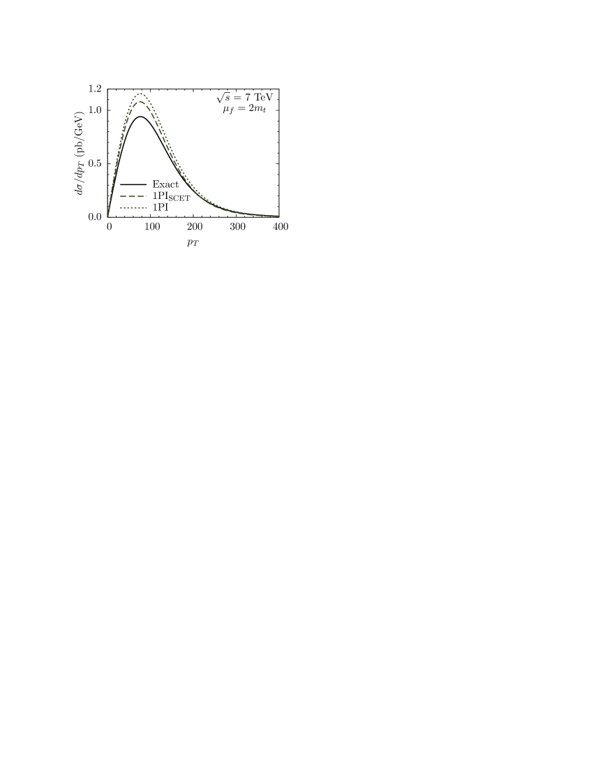
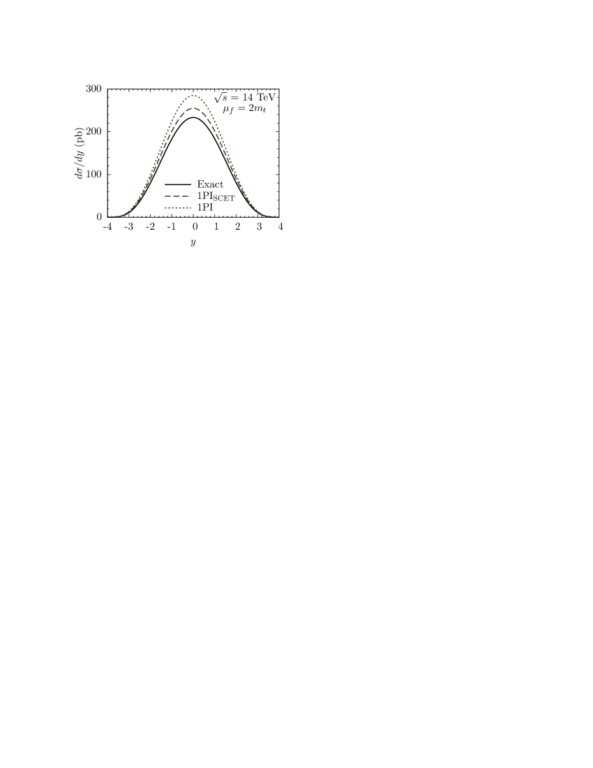
Figure 1: The transverse-momentum and rapidity distributions at NLO at the Tevatron with $\sqrt{s}=1.96$ TeV and at the LHC with $\sqrt{s}=7$ and 14 TeV.

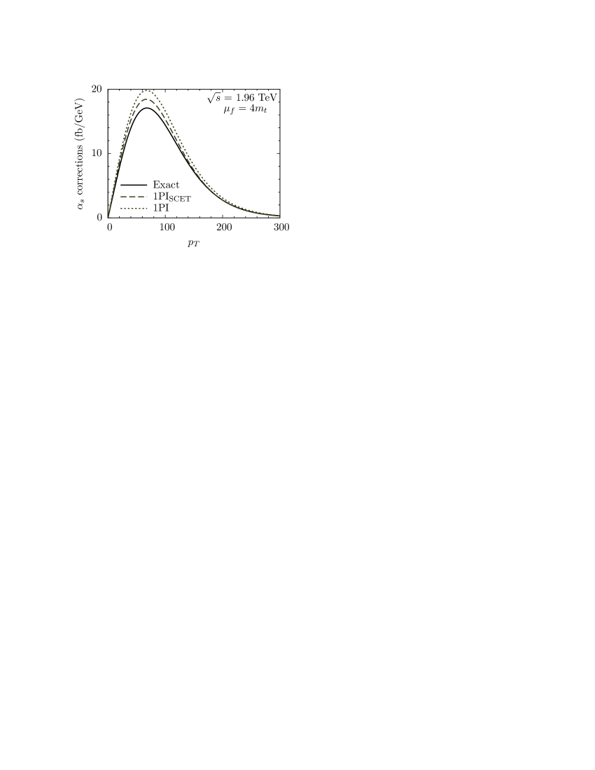
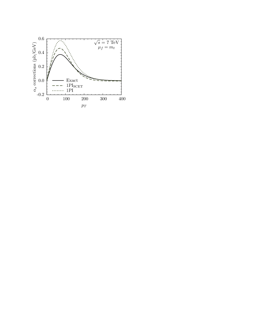
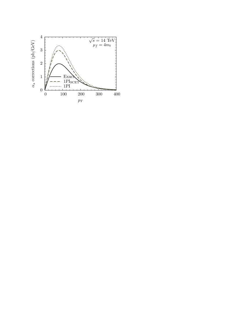
Figure 2: The NLO corrections to $d\sigma/dp_{T}$.

Our first test of the threshold expansion in 1PI kinematics is to compare its predictions for the transverse-momentum and rapidity distributions with the exact ones at NLO in QCD. In other words, we study whether the leading singular pieces in the 1PI or $\text{1PI}_{\text{SCET}}$ threshold expansions provide a good approximation to the exact NLO hard-scattering kernels, so that the power corrections contained in the parentheses of the second term in (4) are small. The results of this comparison can be found in Figure 1, where the transverse-momentum and rapidity distributions at the Tevatron and the LHC with $\sqrt{s}=7$ and 14 TeV are displayed, for the choice $\mu_{f}=2m_{t}$. To compute the exact QCD corrections we rely on the Monte Carlo programs MCFM [76] and an internal NLO version of MadGraph/MadEvent [77, 78], whereas to implement the leading pieces of the threshold expansion in $\text{1PI}_{\text{SCET}}$ and 1PI we have used the procedure described in Section 4. All inputs, including PDFs and $m_{t}$, can also be found in that section. It is obvious from the figures that the $\text{1PI}_{\text{SCET}}$ approximation does better than the 1PI approximation in reproducing the exact QCD results. Since the three curves differ only through the NLO corrections to the hard-scattering kernels, we can compare them much better if we isolate these pieces. We have done so for the $p_{T}$ distribution in Figure 2, in this case for two different values of $\mu_{f}$. We then see that at the Tevatron the $\text{1PI}_{\text{SCET}}$ approximation works remarkably well over the full range of $\mu_{f}$. At the LHC, the $\text{1PI}_{\text{SCET}}$ approximation reasonably reproduces the correction at $\mu_{f}=m_{t}$, but does relatively poorly in reproducing the correct $\mu_{f}$ dependence. The 1PI approximation significantly overestimates the true result at all three values of $\mu_{f}$, both at the Tevatron and at the LHC.

Given that the numerical differences between the $\text{1PI}_{\text{SCET}}$, 1PI, and exact results are due solely to subleading terms as $s_{4}\to 0$, we conclude that power corrections to the pure threshold expansion can be sizeable at NLO. At the Tevatron, where the $q\bar{q}$ channel gives the largest contributions, the extra terms related to $L_{4}$ included in $\text{1PI}_{\text{SCET}}$ account for the dominant power corrections. They are also important at the LHC, where the $gg$ channel dominates, but so are other corrections, which cannot be obtained in our formalism.

We have focused on the region of $p_{T}$ where the differential cross section is largest. In principle, our results can also be used to predict the high-$p_{T}$ tail of the distribution. In the limit $m_{\perp}\to\sqrt{s}/2$, for instance, $s_{4}\to 0$, so threshold expansion is bound to work well when compared to the exact NLO result. However, in such kinematic regions the differential cross section is so small that it is essentially unobservable, and the top-quark is so highly boosted that $m_{t}\ll\sqrt{\hat{s}}$, so the power counting in the effective theory would need to be modified. A more interesting region would be up to around $400$ GeV at the Tevatron, and up to around a TeV at the LHC. We will include the higher-$p_{T}$ region for the Tevatron in the phenomenological studies. For the LHC, however, $s_{4}$ can be on average rather large at such values of $p_{T}$, so power corrections to the $gg$ and $qq$ channels can become significant, and the $qg$ channel can also give non-negligible contributions. Given these problems, we will not study the high-$p_{T}$ distributions at the LHC.

This simple NLO study is instructive, but in the end the real issue is how well the threshold approximation is expected to work at NNLO. On the one hand, at NNLO one encounters plus-distributions enhanced by up to three powers of logarithms, so it is not unreasonable to expect that the power corrections are of less relative importance than at NLO. On the other hand, at NLO the coefficients multiplying both the $P_{n}$ distributions and $\delta$-function terms are known exactly, while at NNLO only those multiplying the $P_{n}$ distributions are available. It is therefore difficult to anticipate the behavior of the threshold expansion at NNLO based only on its behavior at NLO. However, we can gain additional insights through the studies of the $\beta$ distribution in the next subsection.

5.2 The $\bm{\beta}$ distribution and total cross section

The differential cross section with respect to $\beta=\sqrt{1-4m_{t}^{2}/\hat{s}}$ can be expressed as

$$\frac{d\sigma}{d\beta}=\frac{1}{s}\frac{8\beta}{(1-\beta^{2})^{2}}\sum_{ij}\,ff_{ij}\bigg{(}\frac{\hat{s}}{s},\mu_{f}\bigg{)}\,\alpha_{s}^{2}\,f_{ij}\bigg{(}\frac{4m_{t}^{2}}{\hat{s}},\mu_{f}\bigg{)}\,.$$ (54)

The coefficient functions $f_{ij}$ are proportional to the total partonic cross sections, and are obtained from our results by comparison with (4). We define expansion coefficients for these functions as

$$f_{ij} =f_{ij}^{(0)}+4\pi\alpha_{s}f_{ij}^{(1)}+\left(4\pi\alpha_{s}\right)^{2}\left[f_{ij}^{(2,0)}+f_{ij}^{(2,1)}\ln\frac{\mu_{f}^{2}}{m_{t}^{2}}+f_{ij}^{(2,2)}\ln^{2}\frac{\mu_{f}^{2}}{m_{t}^{2}}\right]+\dots\,.$$ (55)

This differential cross section is not measured experimentally, but from the theoretical perspective it is convenient because answers for the partonic cross section are known analytically to NLO [18], and for the functions $f_{ij}^{(2,1)}$ and $f_{ij}^{(2,2)}$ multiplying the scale-dependent logarithms to NNLO [50]. Moreover, this cross section is calculable in both 1PI and PIM kinematics, so it gives us a way of directly comparing the threshold expansion and power corrections for these two cases. The results must agree in the limit $\beta\to 0$, since in that case gluon emission is soft, but beyond that they receive a different set of power corrections, so the agreement of the two approximations with each other is one way of testing whether these power corrections are under control.

We begin with a study of the NLO corrections, similar to that performed for the $p_{T}$ distribution in the previous section. In this case, however, we can also include the results from PIM kinematics, which we calculate using the expressions in [55]. In Figure 3 we compare results for the $\alpha_{s}$ correction to (54) obtained within the different expansions. In contrast to the $p_{T}$ spectrum, we compare the quark and gluon channels separately and look at the corrections in a kinematic range from the production threshold at $\beta=0$ to the machine threshold at $\beta_{\rm max}=\sqrt{1-4m_{t}^{2}/s}$. As anticipated from the results of the previous section, the $\text{1PI}_{\text{SCET}}$ approximation works quite well in the $q\bar{q}$ channel, but somewhat worse in the $gg$ channel, especially at the LHC. The 1PI results overestimate the exact corrections in all cases. As for the results in PIM kinematics, they are lower than the exact results in all cases, but the power-suppressed terms included in $\text{PIM}_{\text{SCET}}$ bring the leading terms in the threshold expansion closer to the full result. The $\text{PIM}_{\text{SCET}}$ approximation is slightly worse than $\text{1PI}_{\text{SCET}}$ in the $q\bar{q}$ channel, and slightly better in the $gg$ channel, but the differences are not major.

As mentioned above, all of the approximations have the same leading-order expansion in the limit $\beta\to 0$. The power-suppressed effects accounting for the differences between the curves start to become noticeable at $\beta\sim 0.2$. After that point, there is more phase space for hard gluon emission and the size of the power corrections increases. Evidently, the subleading terms included in the $\text{1PI}_{\text{SCET}}$ and $\text{PIM}_{\text{SCET}}$ approximations account for these power-suppressed terms in part, although not completely. This is especially noticeable in 1PI kinematics, where the power corrections are generically more important than in PIM kinematics, a point we will return to below. The power corrections become progressively more important at higher values of the collider energy, since then the luminosities are larger at high $\beta$ and the differences in the partonic cross sections in that region are magnified. This is most easily seen by comparing the LHC results at the two different collider energies, where one observes larger gaps between the approximations at 14 TeV than at 7 TeV. A careful examination of the results at the LHC with $\sqrt{s}=14$ GeV also shows a feature not obvious in the other cases: at very high values of $\beta$ close to the endpoint, the exact correction in the $gg$ channel remains a positive number. In fact, the exact NLO correction to the partonic cross section in the $gg$ channel tends to a positive constant at very high $\hat{s}$ [15], while that for the $q\bar{q}$ channel, and also the threshold approximations to the corrections in PIM and 1PI kinematics in both channels, approach zero at high $\hat{s}$. This feature is only visible at the highest collider energy, because otherwise the high-$\beta$ cross section is completely damped by the luminosities. For the same reason, the $qg$ channel, for which the partonic cross section also tends to a positive constant at high $\hat{s}$, can become important at high $\beta$. We show the $\alpha_{s}$ correction from this channel at the LHC in Figure 4, for three different values of $\mu_{f}$ (at the Tevatron, the contribution from this channel is still very small.) For higher values of $\beta$, and especially at lower values of $\mu_{f}$, it can be as important as the $gg$ channel, even though it is suppressed in the limit $s_{4}\to 0$. We discuss this effect at the level of the total cross section in more detail in Section 6.

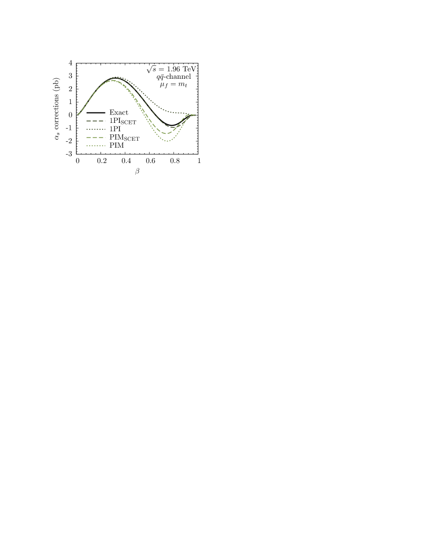
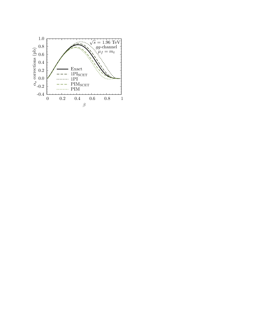
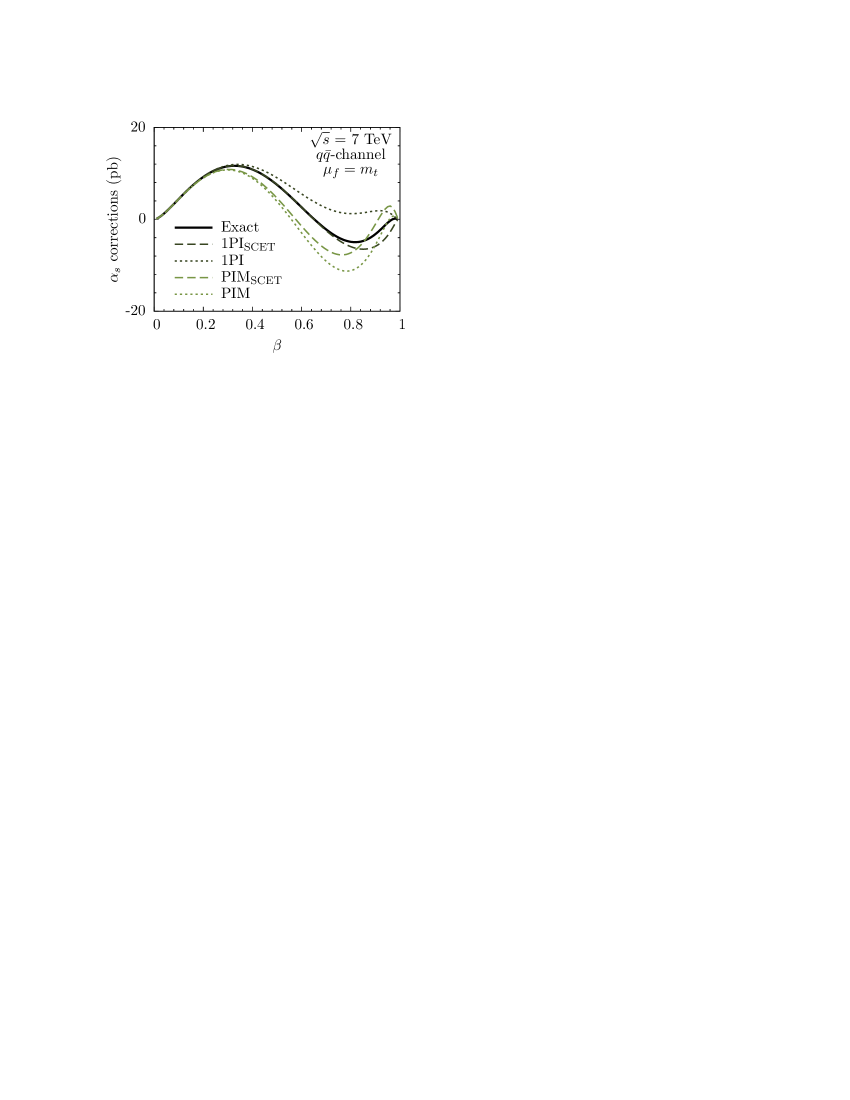
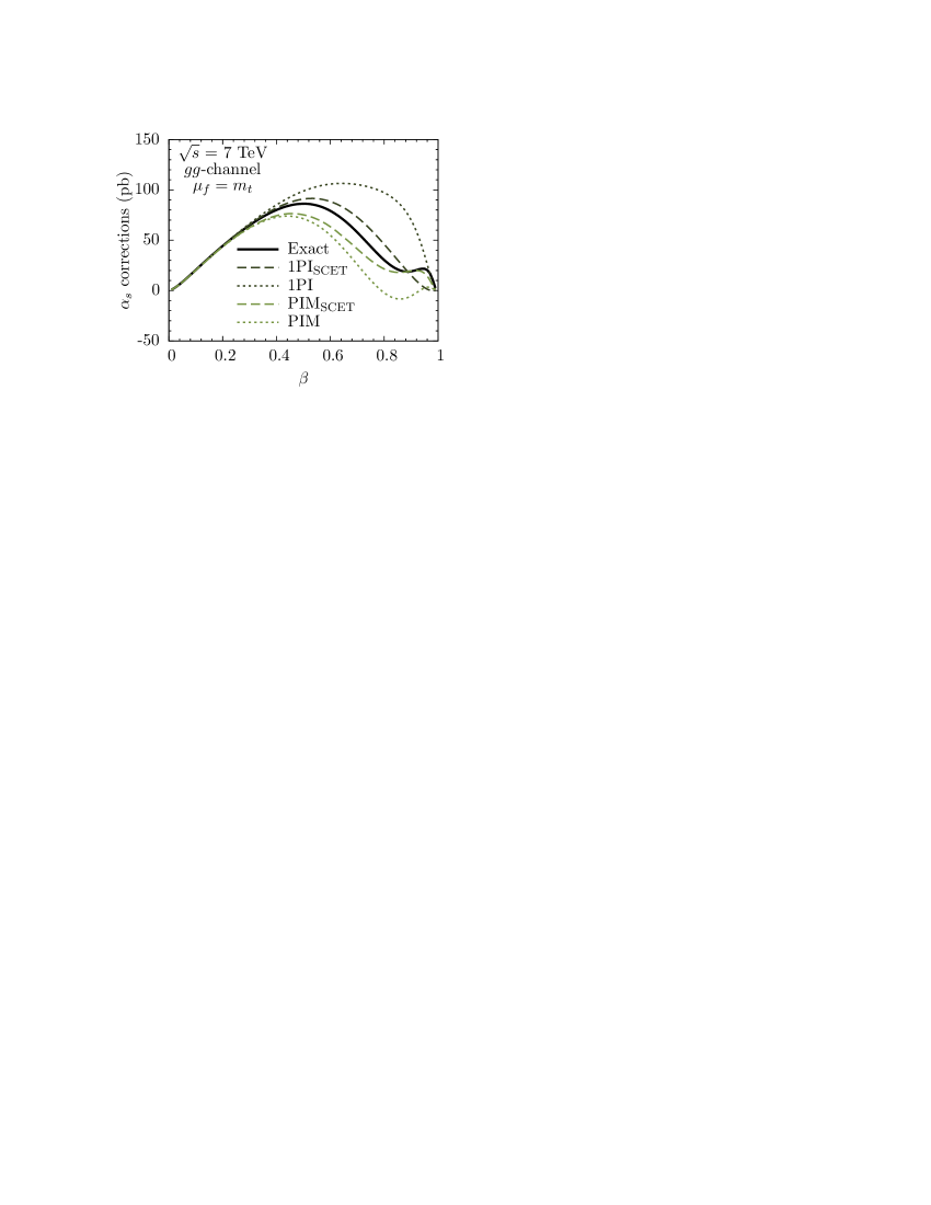
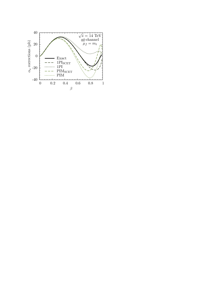
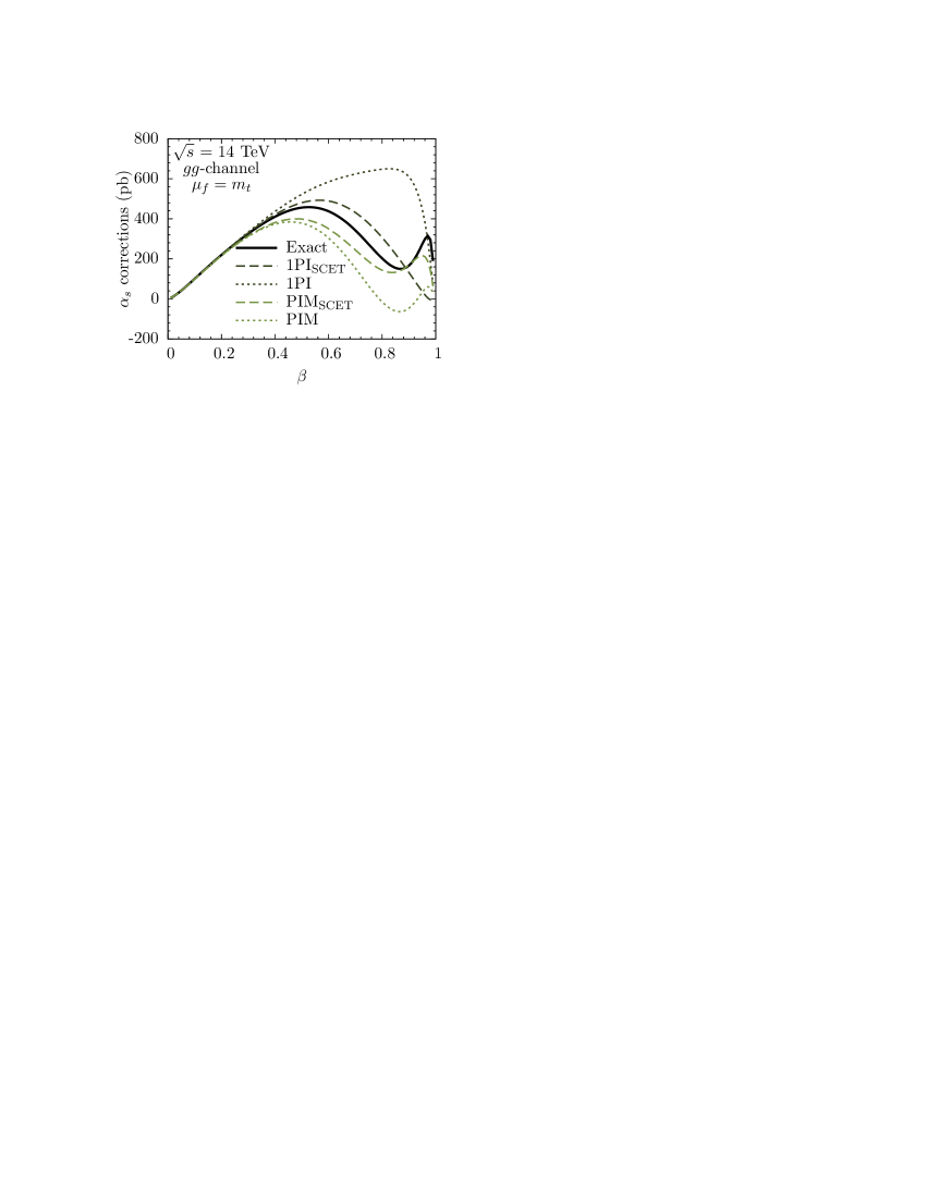
Figure 3: The $\alpha_{s}$ corrections to $d\sigma/d\beta$ for the different approximations mentioned in the text, with $\mu_{f}=m_{t}$.

Figure 4: The $\alpha_{s}$ corrections to $d\sigma/d\beta$ from the $gq$ channel, for $\mu_{f}=m_{t}$ (solid), $\mu_{f}=m_{t}/2$ (dashed) and $\mu_{f}=2m_{t}$ (dotted).

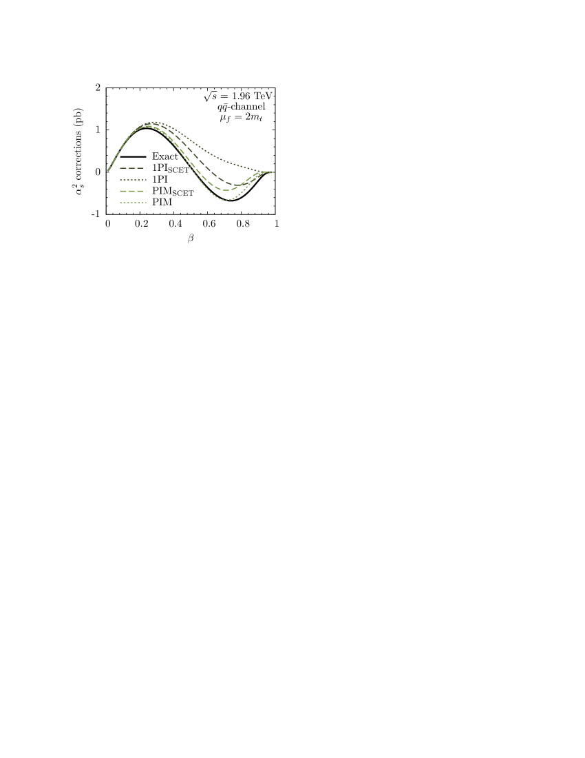
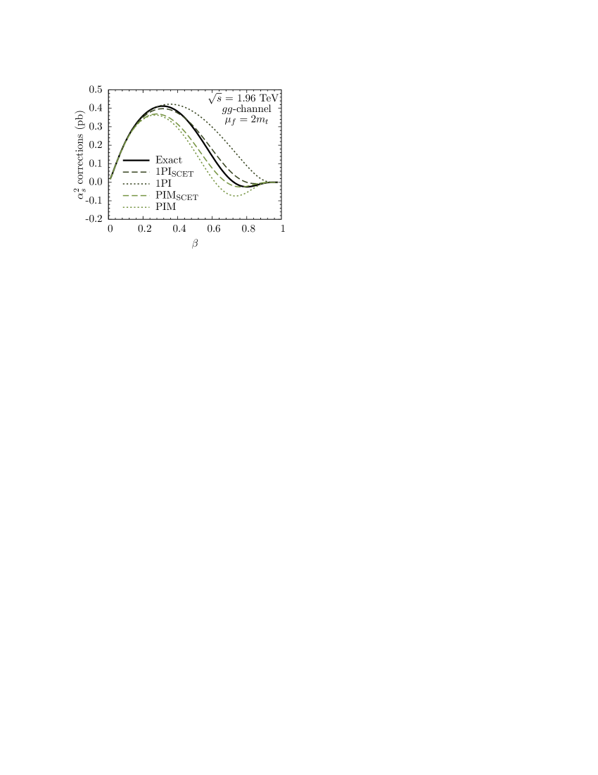
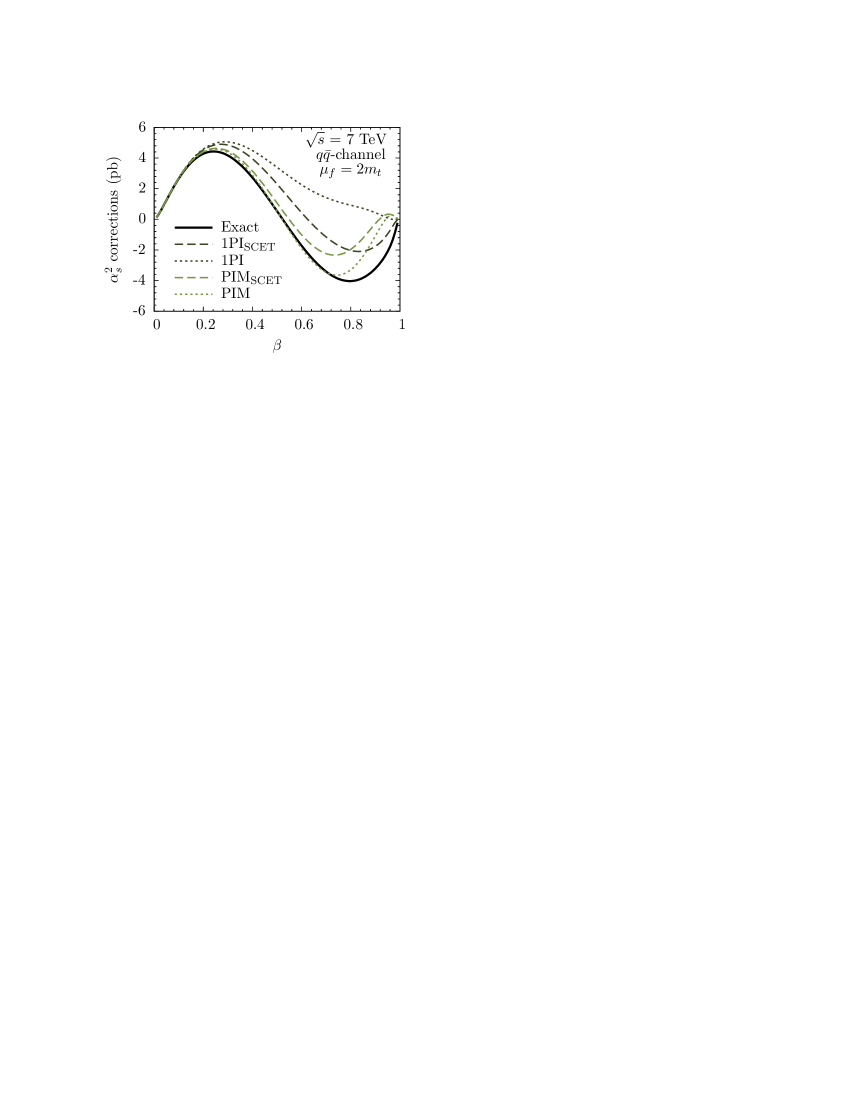
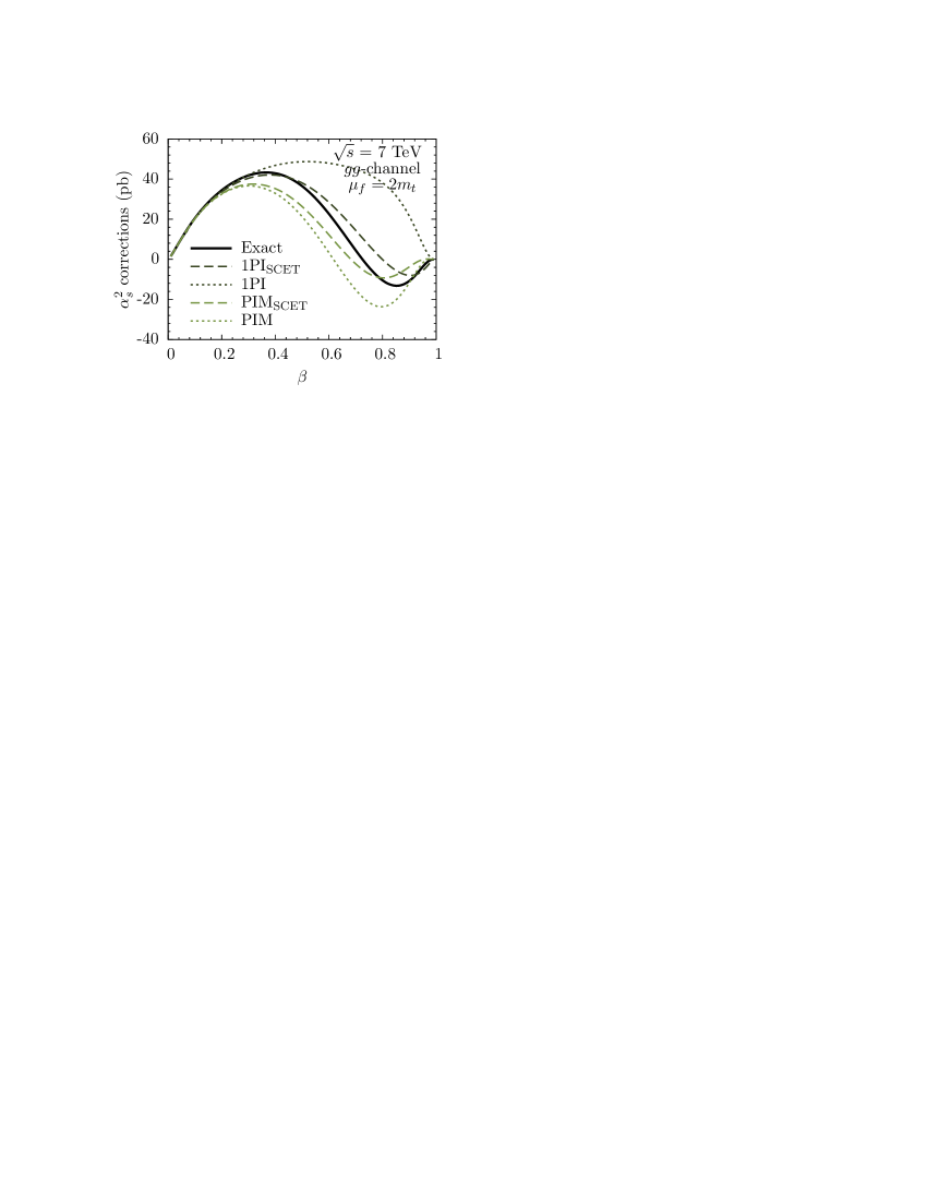
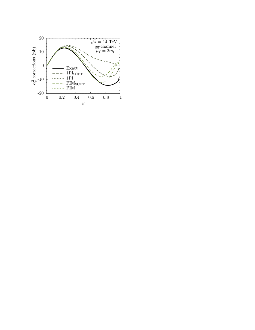
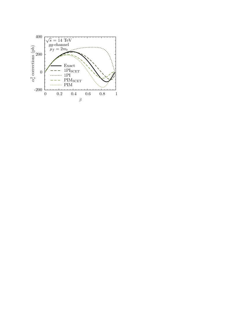
Figure 5: The $\alpha_{s}^{2}$ corrections to $d\sigma/d\beta$ obtained by dropping the scale-independent piece $f^{(2,0)}$ in (55), for $\mu_{f}=2m_{t}$. The exact result is the black line, the dashed red line $\text{1PI}_{\text{SCET}}$, the dotted red line 1PI, the dashed blue line $\text{PIM}_{\text{SCET}}$, and the dotted blue line PIM.

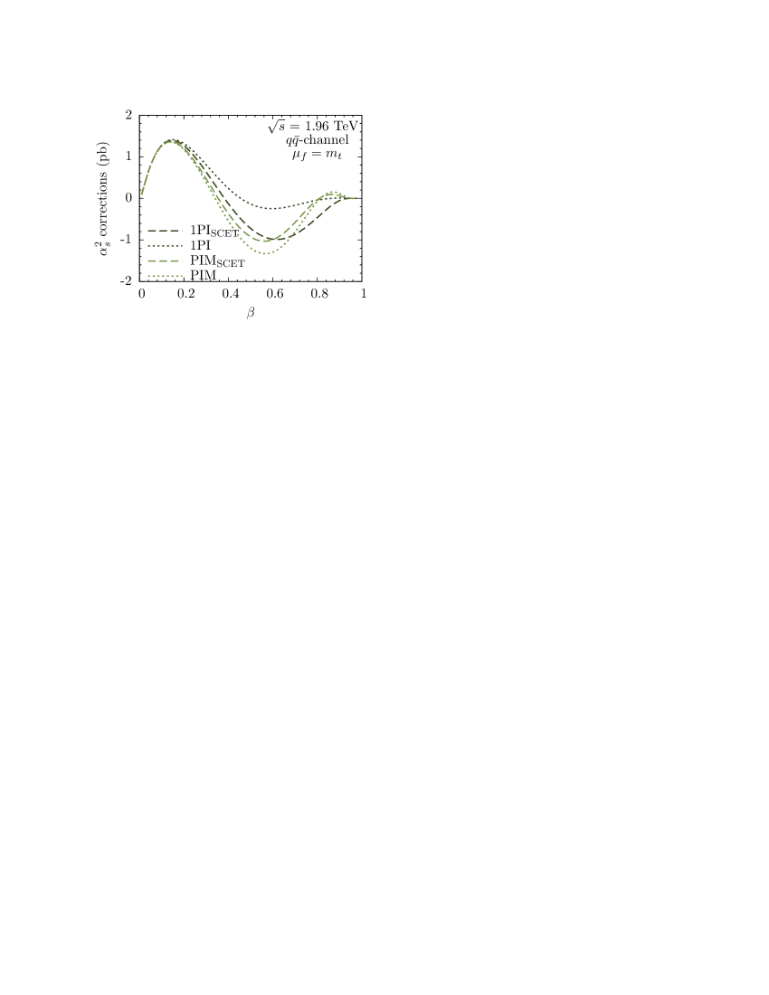
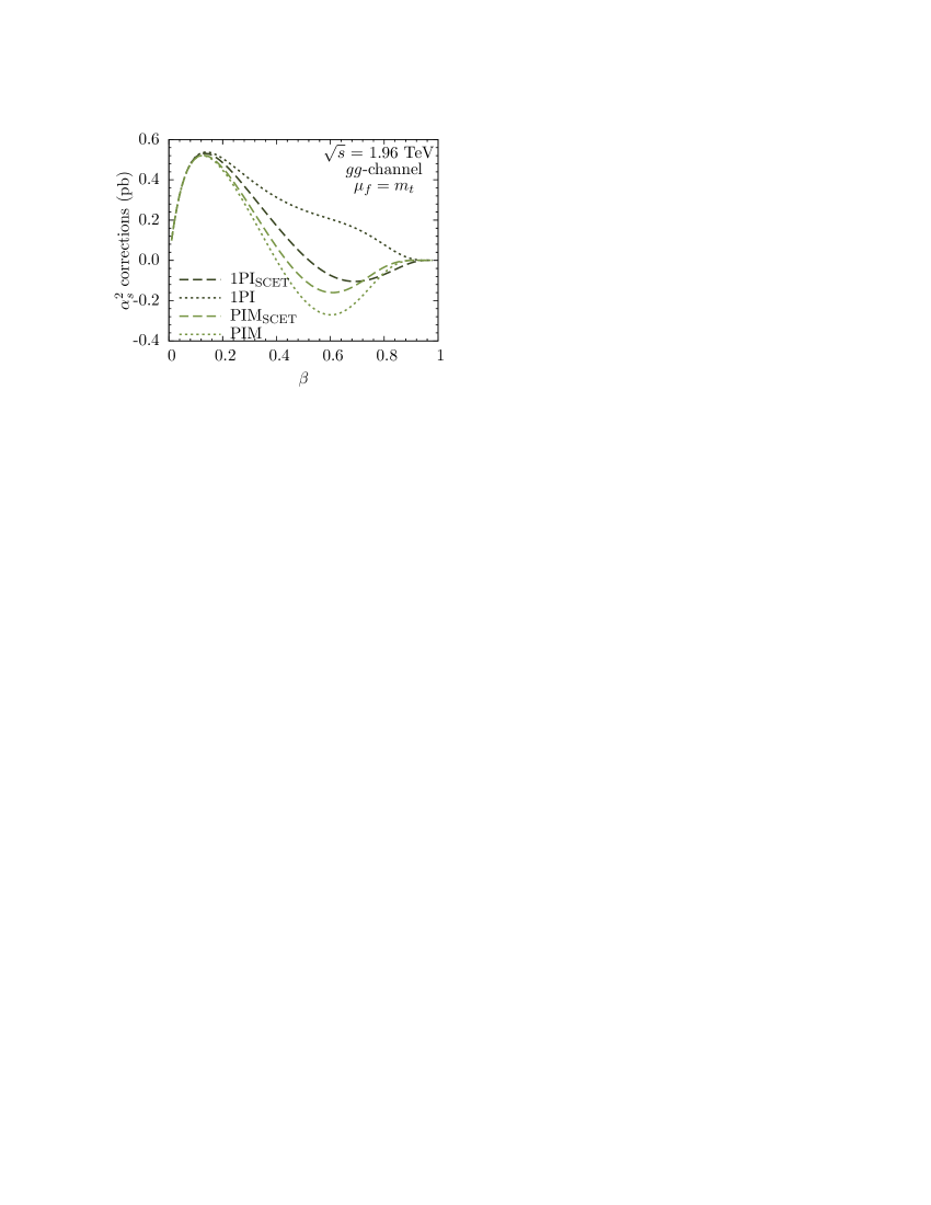
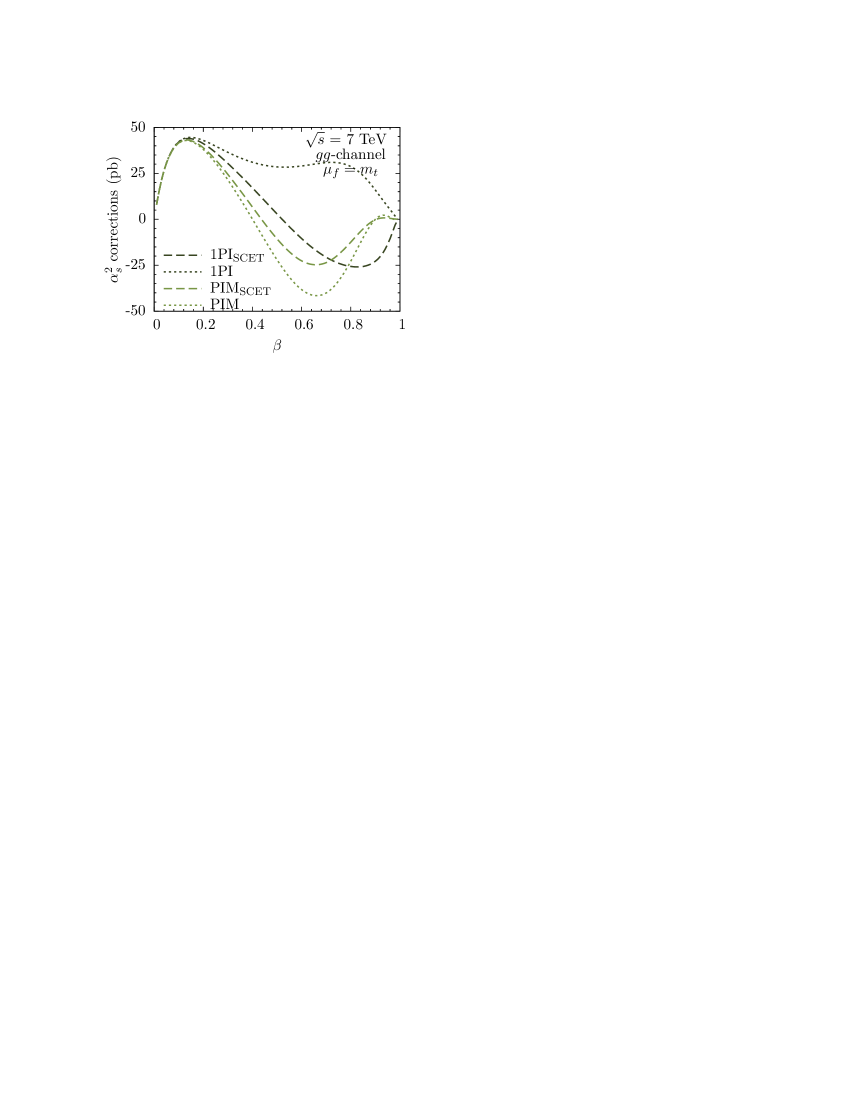
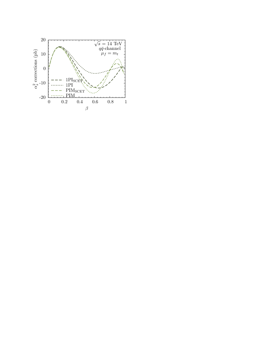
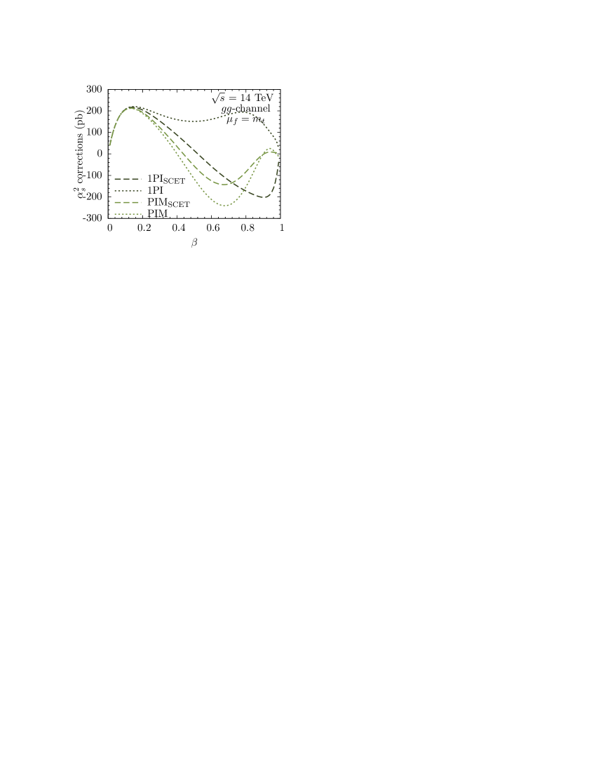
Figure 6: The $\alpha_{s}^{2}$ corrections to $d\sigma/d\beta$ arising from the scale-independent piece, for $\mu_{f}=m_{t}$.

In contrast to the transverse-momentum and rapidity distributions, for which little is known beyond NLO, for the $\beta$ distribution we can also perform some comparisons with other results at NNLO. First of all, results for the $\beta$ distribution at the same level of NNLO approximation, but in PIM kinematics, were obtained in [55], and the agreement of these results with each other gives some information about the size of power-suppressed terms. In addition, the NNLO corrections proportional to the scale-dependent logarithmic terms in the $\beta$ spectrum (54) are known exactly [50]. This gives us an opportunity to also compare both types of kinematics with an exact result beyond NLO.

The NNLO corrections proportional to the scale-dependent logarithmic terms in the $\beta$ distribution (54) within different approximations are shown in Figure 5. The results are obtained by dropping the scale-independent coefficient $f^{(2,0)}$ from (55). Since these contributions would vanish for $\mu_{f}=m_{t}$, we have chosen in this case $\mu_{f}=2m_{t}$ instead. We have evaluated the exact results in QCD using the formulas from [50], and the $\text{PIM}_{\text{SCET}}$ and PIM results using those from [55]. To obtain the threshold expansions for this comparison, we have differed from our normal scheme for including the NNLO corrections described at the end of Section 3 by including the $\mu$-dependent pieces of the two-loop hard function, and by rewriting all $\mu$-dependent logarithms in the form $\ln(m_{t}^{2}/\mu^{2})$. Concerning the agreement between the 1PI approximations and the exact results, one sees the same qualitative behavior as at NLO. The $\text{1PI}_{\text{SCET}}$ results are consistently a better approximation than the 1PI results, especially at the LHC, where the power corrections are large at higher values of $\beta$. As for the PIM results, the $\text{PIM}_{\text{SCET}}$ approximation fares slightly better than the PIM results in the gluon channel, but slightly worse in the quark channel. In any case, the differences between the $\text{PIM}_{\text{SCET}}$ and PIM results are much smaller than those between the $\text{1PI}_{\text{SCET}}$ and 1PI results, which can be taken as an indication that the power corrections are smaller in PIM than in 1PI kinematics. However, once the extra corrections unique to the $\text{1PI}_{\text{SCET}}$ scheme are taken into account, the results in these two types of kinematics are very much compatible with one another and provide a good approximation to the exact results.

The NNLO corrections from the scale-independent pieces $f^{(2,0)}$ to the $\beta$ spectrum (54) within the different PIM and 1PI approximations are shown in Figure 6, for the choice $\mu_{f}=m_{t}$. For these pieces it is not possible to make a comparison with an exact result, but we can make a couple of comments based on the agreement of the different approximations with each other. As before, the difference between the two PIM schemes is small compared to that between the two 1PI schemes, indicating that the power corrections in PIM kinematics are smaller, and the difference between the $\text{1PI}_{\text{SCET}}$ and $\text{PIM}_{\text{SCET}}$ results are much reduced compared to the difference between the 1PI and PIM results. In general, the NNLO corrections in the 1PI approximation are much larger than any of the others.

The explicit results from these studies all point to the fact that 1PI kinematics is more susceptible to power-suppressed effects than PIM kinematics. We can gain more insight into this observation through a very simple analysis. As discussed in Section 3, the leading power corrections in 1PI kinematics are related to the partonic expansion parameter $\lambda=E_{s}/m_{t}$, where $2E_{s}\sim s_{4}/\sqrt{m_{t}^{2}+s_{4}}$ is the energy of extra soft radiation in the partonic scattering process. For the case of PIM kinematics, the equivalent parameter is $\lambda=E^{\rm PIM}_{s}/M$, where $2E^{\rm PIM}_{s}=M(1-z)/\sqrt{z}$. We can quantify in part the relative size of these parameters as a function of $\beta$ by evaluating the mean value

$$\Braket{\lambda}_{\rm 1PI}=\left.\int_{t_{1}^{\text{min}}}^{t_{1}^{\text{max}}}d\hat{t}_{1}\int_{0}^{s_{4}^{\text{max}}}ds_{4}\left(\frac{s_{4}}{2m_{t}\sqrt{m_{t}^{2}+s_{4}}}\right)\right/\int_{t_{1}^{\text{min}}}^{t_{1}^{\text{max}}}d\hat{t}_{1}\int_{0}^{s_{4}^{\text{max}}}ds_{4}$$ (56)

in 1PI kinematics, where the appropriate integration range can be read off from (4), and the analogous expression

$$\Braket{\lambda}_{\rm PIM}=\left.\int_{4m_{t}^{2}/\hat{s}}^{1}dz\left(\frac{1-z}{2\sqrt{z}}\right)\right/\int_{4m_{t}^{2}/\hat{s}}^{1}dz$$ (57)

in PIM kinematics. The results are shown in Figure 7. In the 1PI scheme, there is a sharp growth in the average value of the “small” parameter $\lambda$ with increasing $\beta$. The expansion parameter in the PIM scheme also increases as a function of $\beta$, but not as quickly. Note that this behavior of the partonic expansion parameter $\lambda$ does not translate directly into correspondingly large corrections to the threshold expansion for the physical cross sections. The singular distributions in $s_{4}$ or $(1-z)$ still enhance the region where $\lambda$ is small, even if the integration range covers regions where it is not, and the regions of $\beta$ closer to the endpoint are damped by the parton luminosities. However, given the results of the figure, it is not surprising that the power corrections are generally larger in 1PI than in PIM kinematics, and that they are especially important at the LHC, where the parton luminosities are larger at higher values of $\beta$.

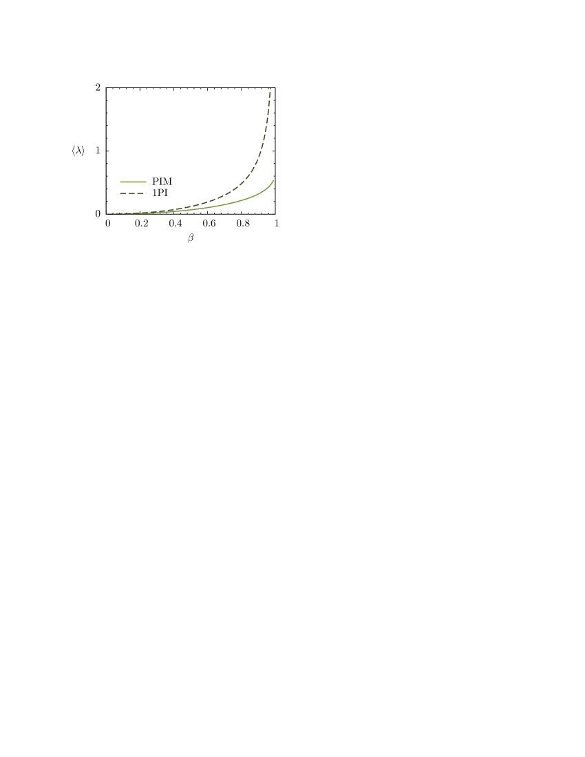
Figure 7: Mean value of the “small” parameter $\lambda$, where $\lambda=(1-z)/(2\sqrt{z})$ in PIM and $\lambda=s_{4}/(2m_{t}\sqrt{m_{t}^{2}+s_{4}})$ in 1PI kinematics.

So far, we have focused on the agreement of the corrections in 1PI or PIM kinematics with the exact QCD results or with each other. We can gain more information by looking at the contributions of the individual terms in the decomposition (39) in the 1PI scheme and also at the analogous contributions in the PIM scheme. The assumption of dynamical threshold enhancement is that contributions from regions of phase space where the partonic expansion parameter $\lambda$ is large, as shown for example in Figure 7, are suppressed due to the properties of the PDFs, so one can expect to see a hierarchy between the different terms in the expansion. In particular, one would expect that the plus-distributions contribute more than the $\delta$-function and of course the power-suppressed contributions contained in $R$.

The exact structure of contributions to the total cross section from the different terms are shown in Table 2, for the choice $\mu_{f}=m_{t}$. Generally speaking, the $P_{i}$ distributions are indeed enhanced compared to the other terms. In fact, the NNLO contributions from $P_{3}$ can be as large as the NLO contributions from $P_{1}$. However, in both 1PI and PIM kinematics, there are large cancellations between the different terms, so that the total NNLO correction turns out to be small. In PIM kinematics, this happens at the level of the distributions, and to a lesser extent between the $\delta$-function and $R$ terms, which seem to be generically smaller than the other terms. In 1PI kinematics, the $\delta$-function terms and especially the power-suppressed terms in $R$ are relatively larger than in PIM. We emphasize that the results for the coefficients of the $P_{i}$ distributions are exact, so a full NNLO calculation will change only the $\delta$-function and $R$ pieces, moreover in such a way that the cross section from both types of kinematics agrees exactly. The numbers above suggest that these terms are relatively small in PIM kinematics, because of threshold enhancement, so in order to preserve the good agreement between the two types of kinematics they would also need to be small in 1PI kinematics. In that case the terms already included in our calculation are the dominant ones at NNLO, although this can only be confirmed through the full NNLO results.

			$P_{3}$	$P_{2}$	$P_{1}$	$P_{0}$	$\delta$	$R$	sum
Tevatron	$\text{1PI}_{\text{SCET}}$	$\delta\sigma^{(1)}_{q\bar{q}}$			1.1	0.30	$-0.06$	$-0.38$	0.94
		$\delta\sigma^{(2)}_{q\bar{q}}$	0.57	0.39	$-0.09$	$-0.19$	$-0.37$	$-0.31$	$0.01$
		$\delta\sigma^{(1)}_{gg}$			0.32	0.08	$-0.11$	$-0.06$	0.45
		$\delta\sigma^{(2)}_{gg}$	0.39	0.18	$-0.07$	$-0.14$	$-0.12$	$-0.12$	0.14
	$\text{PIM}_{\text{SCET}}$	$\delta\sigma^{(1)}_{q\bar{q}}$			1.2	$-0.67$	$-0.11$	0.20	0.64
		$\delta\sigma^{(2)}_{q\bar{q}}$	0.64	$-0.24$	$-0.26$	$-0.16$	$-0.08$	0.11	0.02
		$\delta\sigma^{(1)}_{gg}$			0.48	$-0.24$	0.12	0.03	0.38
		$\delta\sigma^{(2)}_{gg}$	0.60	$-0.31$	$-0.11$	$-0.11$	$-0.08$	0.04	0.10
LHC14	$\text{1PI}_{\text{SCET}}$	$\delta\sigma^{(1)}_{q\bar{q}}$			18	1	$-2$	$-9$	7
		$\delta\sigma^{(2)}_{q\bar{q}}$	8.1	2.9	$-1.6$	$-0.6$	$-5.4$	$-4.6$	$-1.1$
		$\delta\sigma^{(1)}_{gg}$			280	14	124	$-125$	292
		$\delta\sigma^{(2)}_{gg}$	296	83	$-20$	$-35$	$-160$	$-149$	16
	$\text{PIM}_{\text{SCET}}$	$\delta\sigma^{(1)}_{q\bar{q}}$			11	$-9$	$-1$	5	6
		$\delta\sigma^{(2)}_{q\bar{q}}$	5.5	$-2.8$	$-1.7$	$-1.0$	$-1.3$	1.1	$-0.1$
		$\delta\sigma^{(1)}_{gg}$			250	$-189$	120	60	240
		$\delta\sigma^{(2)}_{gg}$	287	$-194$	$-41$	$-60$	$-10$	37	19

Table 2: Corrections in pb from the different types of distributions at NLO and NNLO, for $\mu_{f}=m_{t}$.

6 Phenomenology

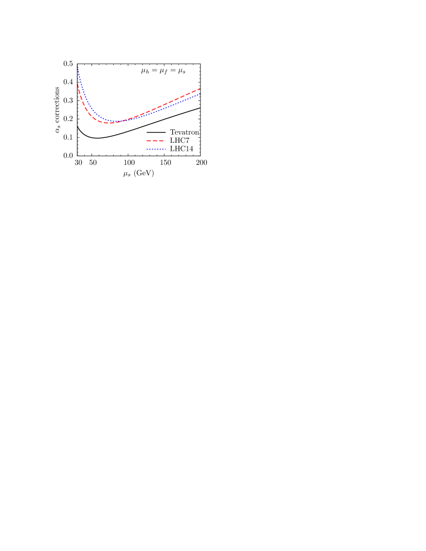
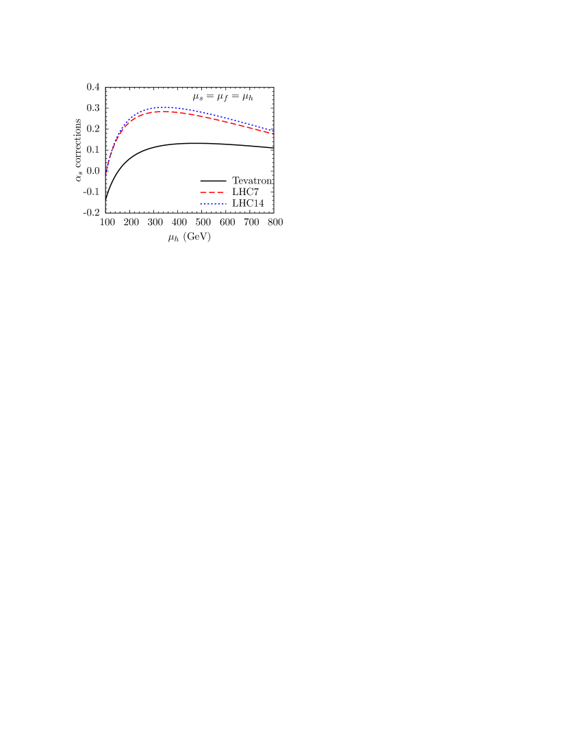
Figure 8: The one-loop correction from the soft function (left) and the hard function (right) to the total cross section, divided by the leading-order result. The solid black line is for the Tevatron, the dashed red line for LHC7, and the dotted blue line for LHC14.

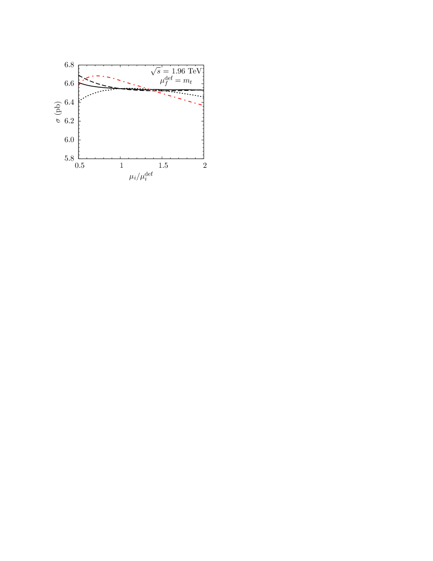
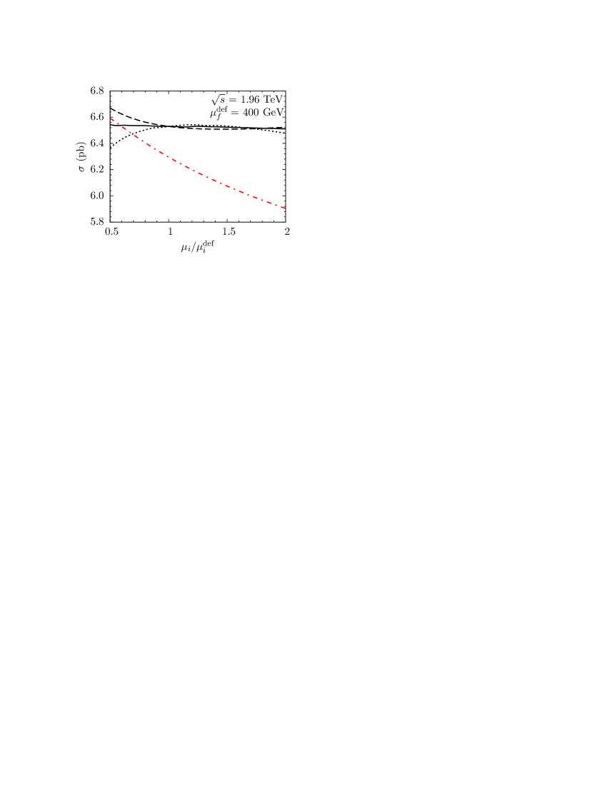
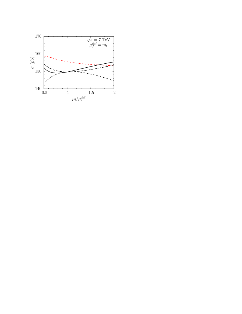
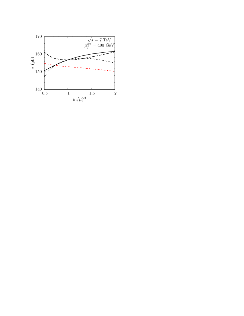
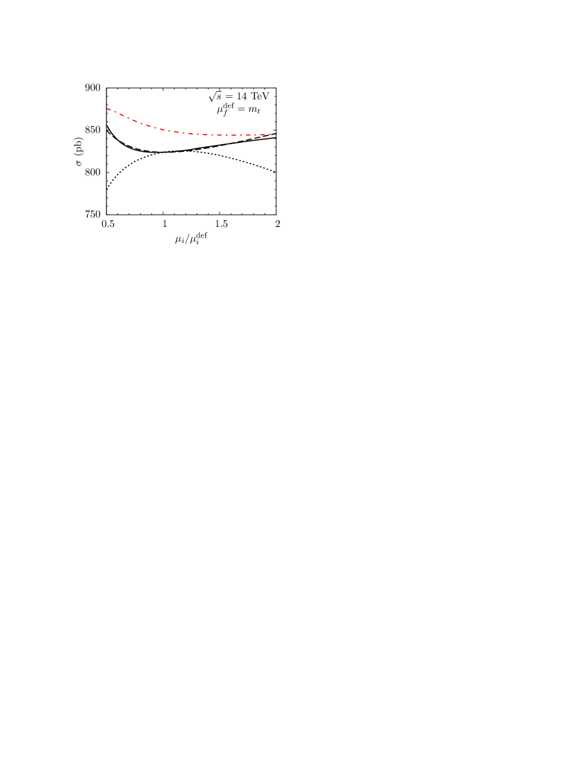
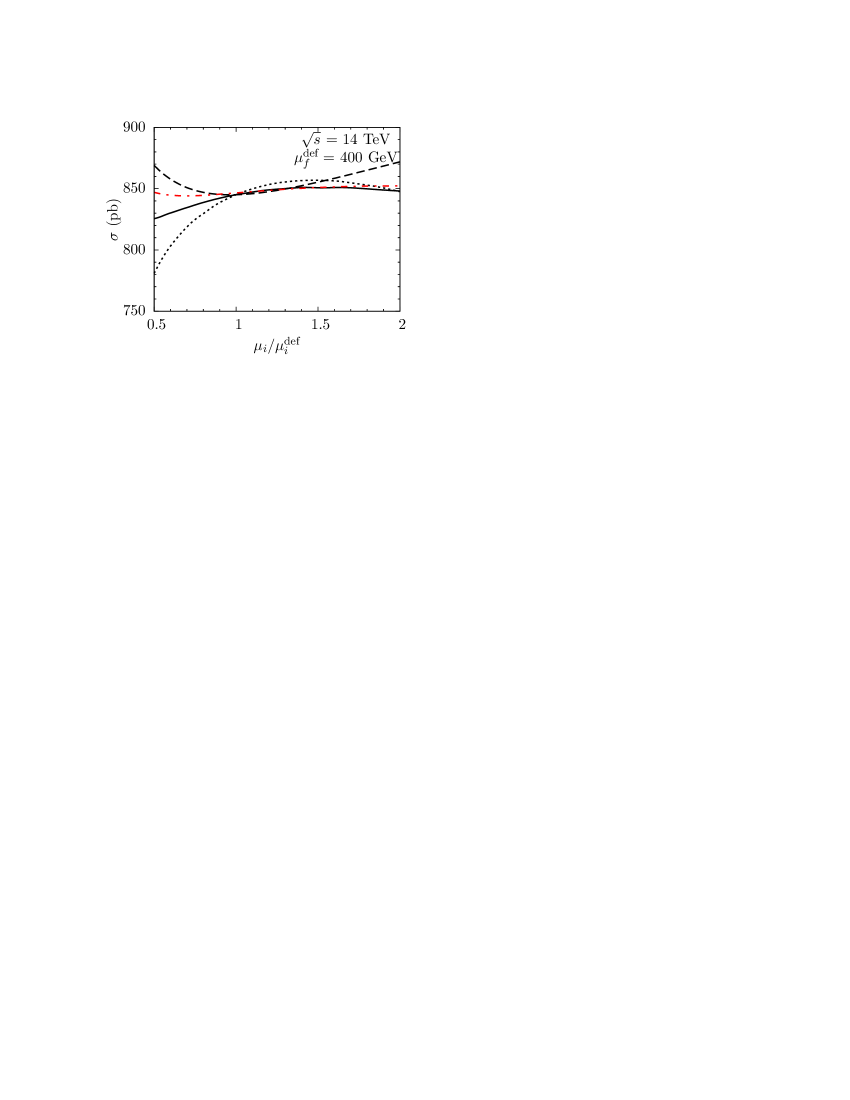
Figure 9: Dependence of the cross section at NLO+NNLL and approximate NNLO in $\text{1PI}_{\text{SCET}}$ on the scales $\mu_{f},\mu_{s}$, and $\mu_{h}$. The dot-dashed red lines show the dependence of the cross section on $\mu_{f}$ in approximate NNLO. The dependence of the cross section on the scales at NLO+NNLL order is represented by the solid black lines ($\mu_{f}$), the dashed black lines ($\mu_{s}$), and the dotted black lines ($\mu_{h}$).

We now have all the ingredients in place to present detailed phenomenological results for the $p_{T}$ and rapidity distributions, the forward-backward asymmetry at the Tevatron, and the total cross section. Before doing so, we review some of the necessary inputs. We have already described our scheme for evaluating the approximate NNLO corrections in Section 3, and that for evaluating the formulas at threshold in Section 4, where our treatment of PDFs and the top-quark mass was also summarized. In addition, we must specify the choice of the matching scales $\mu_{s}$ and $\mu_{h}$, and of the factorization scale $\mu_{f}$.

We begin by discussing our method for determining an appropriate choice of the soft scale $\mu_{s}$. From theoretical arguments, we expect that the perturbative expansion of the soft function should be well-behaved at a scale characteristic of the energy of the real soft radiation, which is generally smaller than the hard scales $m_{t}$ and $\sqrt{\hat{s}}$. As explained in Section 3.4, a general analysis would determine the soft scale by requiring that the corrections from the soft function to the double-differential spectrum are well behaved, after integration over the partonic variables. We have performed such an analysis for the $p_{T}$ distribution and found reasonable results at the Tevatron. This is also the case for the LHC at lower values of $p_{T}$, where the differential cross section is large. As long as we study a relatively modest range in $p_{T}$, an equally valid procedure for determining the soft scale is to study the corrections to the total cross section as a function of $\mu_{s}$. This automatically samples the regions of phase-space where the double-differential cross section is largest. We show the results of such an analysis in Figure 8. To isolate the $\alpha_{s}$ correction from the soft function shown there, we pick out the piece of the NNLL approximation to the hard scattering kernels arising from $\widetilde{\bm{s}}^{(1)}$, evaluate the total cross section using only this piece, and divide the result by that at NLL, working in the $\text{1PI}_{\text{SCET}}$ scheme. We furthermore make the scale choice $\mu_{f}=\mu_{h}=\mu_{s}$, which amounts to looking at the correction at NLO in fixed-order. As seen from the figure, a well-defined minimum in the soft correction appears for $\mu_{s}\sim 60$ GeV at the Tevatron, $\mu_{s}\sim 80$ GeV at the LHC with $\sqrt{s}=7$ GeV, and $\mu_{s}\sim 90$ GeV at the LHC with $\sqrt{s}=14$ GeV. We will use these as the default choices of $\mu_{s}$ in the rest of this section, both for the total cross section and for differential distributions.

One can apply this same procedure to determine an appropriate choice of the hard scale. Since the hard function is the same in PIM and 1PI kinematics, we first recall the analysis of [55], where it was argued that $\mu_{h}=M$ is a reasonable default value. Translated to 1PI kinematics, this would imply the choice $\mu_{h}=\sqrt{\hat{s}}$. The actual result for the $\alpha_{s}$ correction to the total cross section arising from the hard function as a function of $\mu_{h}$ is shown in the right panel of Figure 8. We isolate this correction as we did for the soft function, except for this time we pick out the piece of the NNLL cross section proportional to $\bm{H}^{(1)}$, and examine the result as a function of $\mu_{h}$. As for the analysis with the soft function, we make the choice $\mu_{f}=\mu_{h}=\mu_{s}$. At lower values of $\mu_{h}$ the correction becomes negative and depends strongly on the scale. To avoid sensitivity to that region, we will choose $\mu_{h}=400$ GeV by default, which is close to the average value of $\sqrt{\hat{s}}$ for the total cross section, and in any case will be varied by a factor of two in the error analysis.

For the factorization scale, we will consider the two different choices $\mu_{f}=m_{t}$ and $\mu_{f}=400$ GeV used in [55]. Of course we could also just choose a single, intermediate value of $\mu_{f}$ and vary it in a larger range, but in resummed perturbation theory it is useful to have independent variations of the matching scales $\mu_{h}$ and $\mu_{s}$ for the two different values of $\mu_{f}$. For the differential distributions in the following subsection, on the other hand, we use $\mu_{f}=2m_{t}$ as the central value. A more refined analysis could use other choices, such as $\mu_{f}=m_{\perp}$ for the $p_{T}$ distribution, but since we do not study tails of the distributions we prefer to stick to a single value which is roughly intermediate between the two values used for the total cross section.

We should mention that another method often used to argue for a particular scale choice is to look for areas where the scale dependence of the observable is flat. As part of our analysis below, we show in Figure 9 the dependence of the total cross section on the scales $\mu_{s}$, $\mu_{h}$, and $\mu_{f}$, at NLO+NNLL and approximate NNLO. We note that the scale-dependence of the cross section at NLO+NNLL order is indeed flat close to our default values of $\mu_{s}$ and $\mu_{h}$, and also close to $\mu_{f}=m_{t}$. The approximate NNLO results, on the other hand, do not seem to favor a particular choice of $\mu_{f}$ based on this criteria.

6.1 Rapidity and transverse-momentum distributions

\psfrag{y}[1][90]{$d\sigma/dy$ [fb]}\psfrag{x}{$y$}\psfrag{z}[0.85]{$\sqrt{s}=1.96$\,TeV}\includegraphics[width=186.45341pt]{tev_1960_y_fixed}	\psfrag{y}[1][90]{$d\sigma/dy$ [fb]}\psfrag{x}{$y$ }\psfrag{z}[0.85]{$\sqrt{s}=1.96$\,TeV}\includegraphics[width=186.45341pt]{tev_1960_y_res}
\psfrag{y}[1][90]{$d\sigma/dy$ [pb]}\psfrag{x}{$y$ }\psfrag{z}[0.85]{$\sqrt{s}=7$\,TeV}\includegraphics[width=186.45341pt]{lhc_7000_y_fixed}	\psfrag{y}[1][90]{$d\sigma/dy$ [pb]}\psfrag{x}{$y$ }\psfrag{z}[0.85]{$\sqrt{s}=7$\,TeV}\includegraphics[width=186.45341pt]{lhc_7000_y_res}
\psfrag{y}[1][90]{$d\sigma/dy$ [pb]}\psfrag{x}{$y$ }\psfrag{z}[0.85]{$\sqrt{s}=7$\,TeV}\includegraphics[width=186.45341pt]{lhc_14000_y_fixed}	\psfrag{y}[1][90]{$d\sigma/dy$ [pb]}\psfrag{x}{$y$ }\psfrag{z}[0.85]{$\sqrt{s}=7$\,TeV}\includegraphics[width=186.45341pt]{lhc_14000_y_res}

Figure 10: Left: Fixed-order predictions for the rapidity distribution at LO (light), NLO (darker), and approximate NNLO (dark bands) for the Tevatron (top) and LHC (bottom). Right: Corresponding predictions at NLL (light) and NLO+NNLL (darker bands) in resummed perturbation theory. The width of the bands reflects the uncertainty of the distributions under variations of the matching and factorization scales, as explained in the text.

\psfrag{y}[1][90]{$d\sigma/dp_{T}$ [fb/GeV]}\psfrag{x}{$p_{T}$ [GeV]}\psfrag{z}[0.85]{$\sqrt{s}=1.96$\,TeV}\includegraphics[width=186.45341pt]{tev_1960_pt_fixed}

\psfrag{y}[1][90]{$d\sigma/dp_{T}$ [fb/GeV]}\psfrag{x}{$p_{T}$ [GeV]}\psfrag{z}[0.85]{$\sqrt{s}=1.96$\,TeV}\includegraphics[width=186.45341pt]{tev_1960_pt_res}

Figure 11: Left: Fixed-order predictions for the $p_{T}$ distribution at LO (light), NLO (darker), and approximate NNLO (dark bands) at the Tevatron. Right: Corresponding predictions at NLL (light) and NLO+NNLL (darker bands) in resummed perturbation theory. The width of the bands reflects the uncertainty of the distributions under variations of the matching and factorization scales, as explained in the text.

\psfrag{y}[1][90]{$d\sigma/dp_{T}$ [fb/GeV]}\psfrag{x}{$p_{T}$ [GeV]}\psfrag{z}[0.85]{$\sqrt{s}=1.96$\,TeV}\includegraphics[width=390.25534pt]{p_t-data}

Figure 12: Comparison between our NLO+NNLL predictions, NLO results and recent measurements from the D0 collaboration [79]. The error bands refers to perturbative uncertainties related to scale variations. Furthermore we have enlarged the region of bigger $p_{T}$ for better comparison.

We now present results for the top-quark rapidity and transverse-momentum distributions. We begin by studying rapidity distributions in Figure 10, where we compare results from fixed-order and resummed calculations in the $\text{1PI}_{\text{SCET}}$ scheme at the Tevatron and the LHC with $\sqrt{s}=7$ and 14 TeV. The results within a given perturbative approximation are represented as bands indicating the theoretical uncertainties from scale variations. To make the bands in fixed-order perturbation theory at a given point in $y$, we vary the value of the factorization scale up and down from its default value at $\mu_{f}=2m_{t}$ by a factor of two, and pick out the highest and lowest numbers at that point. To make the bands in resummed perturbation theory, we vary individually $\mu_{f}$, $\mu_{h}$, or $\mu_{s}$ with the others held fixed at their default values, pick out the highest and lowest numbers, and then add the three highest and three lowest numbers in quadrature. The results in the figure clearly show that the higher-order corrections contained in the approximate NNLO and NLO+NNLL formulas tend to reduce the uncertainties due to scale dependence, and slightly raise the central values at a given rapidity to the upper part of the fixed-order NLO band. The error bands for the NLO+NNLL and approximate NNLO results are of similar size at the Tevatron, but at the LHC the approximate NNLO bands are noticeably smaller, a result which we will quantify in more detail when we study the total cross section.

Next, we consider the top-quark transverse-momentum distribution. In this case, we focus our analysis on the Tevatron, where experimental measurements are available. In Figure 11 we show our predictions for this distribution within the different perturbative approximations, comparing the fixed-order and resummed results. As with the rapidity distributions, the higher-order perturbative corrections serve to decrease the scale dependence, and also to slightly raise the central values of the results at a given $p_{T}$. We compare the NLO+NNLL results for the $p_{T}$ distribution with a recent measurement at the Tevatron performed by the D0 collaboration using the lepton+jets channel [79] in Figure 12, showing also the NLO calculation for illustration. Since the D0 analysis uses $m_{t}=170$ GeV, for the purposes of this study we deviate from our default choice and also adopt this value. We observe that the slight increase in the the differential cross section due to resummation leads to a better agreement with the data compared to the NLO predictions. In general, the measured spectrum and the NLO+NNLL theory prediction agree within the errors, both in the shape and the normalization. This is true even at higher values of $p_{T}$, although one should keep in mind that our scale-setting procedure was designed to work in areas where the differential cross section is large, and at $p_{T}\sim 400$ GeV it would also be interesting to perform a more involved analysis where $\mu_{f},\mu_{s}$, and $\mu_{h}$ are chosen as dynamical functions of $p_{T}$.

6.2 The forward-backward asymmetry at the Tevatron

The top-quark pair charge asymmetry is an important observable at the Tevatron. It originates from the difference in the production rates for top and anti-top quarks at fixed scattering angle or rapidity [22, 23]. Due to charge-conjugation invariance in QCD, it can also be interpreted as a forward-backward asymmetry using (9). This asymmetry vanishes at LO in $\alpha_{s}$ and is only about 5%–10% at NLO, so it is potentially sensitive to new physics contributions and has received much interest for that reason.

The forward-backward asymmetry depends on the frame in which it is measured. Experimentally the asymmetry has been measured both in the laboratory frame and in the $t\bar{t}$ rest frame [8, 7]. In [55], we used results from PIM kinematics to calculate the asymmetry to NLO+NNLL and approximate fixed order in the partonic center-of-mass frame, with the aim of improving the NLO fixed-order calculations from [23] and the NLL results from [62]. In what follows we use our results for 1PI kinematics to obtain NLO+NNLL and approximate NNLO predictions directly in the laboratory frame.

	$0.2<\mu_{f}/{\rm TeV}<0.8$		$m_{t}/2<\mu_{f}<2m_{t}$
	$\Delta\sigma_{\rm FB}$ [pb]	$A^{t}_{\text{FB}}$ [%]	$\Delta\sigma_{\rm FB}$ [pb]	$A^{t}_{\text{FB}}$ [%]
NLL, $\text{1PI}_{\text{SCET}}$	0.234${}^{+0.099}_{-0.116}$	4.12${}^{+2.11}_{-2.06}$	0.238${}^{+0.105}_{-0.119}$	4.24${}^{+2.17}_{-2.12}$
NLO leading, $\text{1PI}_{\text{SCET}}$	0.164${}^{+0.077}_{-0.049}$	4.40${}^{+0.38}_{-0.33}$	0.262${}^{+0.141}_{-0.085}$	4.86${}^{+0.46}_{-0.39}$
NLO	0.163${}^{+0.076}_{-0.048}$	4.36${}^{+0.36}_{-0.32}$	0.260${}^{+0.140}_{-0.084}$	4.81${}^{+0.45}_{-0.39}$
NLO+NNLL, $\text{1PI}_{\text{SCET}}$	0.295${}^{+0.026}_{-0.032}$	4.61${}^{+0.27}_{-0.26}$	0.312${}^{+0.027}_{-0.035}$	4.88${}^{+0.20}_{-0.23}$
NNLO approx, $\text{1PI}_{\text{SCET}}$	0.241${}^{+0.023}_{-0.030}$	4.27${}^{+0.31}_{-0.26}$	0.270${}^{+0.037}_{-0.023}$	4.01${}^{+0.54}_{-0.00}$

Table 3: The asymmetric cross section and forward-backward asymmetry at the Tevatron, evaluated at different orders in perturbation theory in the $p\bar{p}$ center-of-mass frame. The errors refer to perturbative uncertainties related to scale variations, as explained in the text.

We define the forward-backward asymmetry as the ratio

$$A^{t}_{\text{FB}}=\frac{\Delta\sigma_{\text{FB}}}{\sigma}\,,$$ (58)

where the asymmetric cross section for the difference between the production of top quarks in the forward and backward directions is

$$\Delta\sigma_{\text{FB}}\equiv\int_{0}^{y_{+}}dy\int_{0}^{p_{T}^{\rm max}}\!dp_{T}\,\frac{d^{2}\sigma^{p\bar{p}\to tX_{\bar{t}}}}{dp_{T}dy}-\int_{-y_{+}}^{0}dy\int_{0}^{p_{T}^{\rm max}}\!dp_{T}\,\frac{d^{2}\sigma^{p\bar{p}\to tX_{\bar{t}}}}{dp_{T}dy}\,,$$ (59)

with

$$y_{+}=\frac{1}{2}\ln\frac{1+\sqrt{1-4m_{t}^{2}/s}}{1-\sqrt{1-4m_{t}^{2}/s}}\,,\qquad p_{T}^{\rm max}=\frac{\sqrt{s}}{2}\sqrt{\frac{1}{\cosh^{2}y}-\frac{4m_{t}^{2}}{s}}\,.$$ (60)

In Table 3, we show the results for the asymmetric cross section and forward-backward asymmetry obtained in different perturbative approximations. In calculating the asymmetry, we first evaluate the numerator and denominator of the ratio $A^{t}_{\text{FB}}=\Delta\sigma_{\text{FB}}/\sigma$ to the order indicated in the table (using our scheme for the PDFs from Table 1), and then further expand the ratio itself, as appropriate at that order. We have obtained the fixed-order NLO results using the formulas from Appendix A of [23] and cross-checked them using MCFM. As seen from the table, the higher-order corrections contained in the NLO+NNLL and approximate NNLO formulas stabilize the asymmetric cross section at values not far from the NLO calculation with $\mu_{f}=m_{t}$. The forward-backward asymmetry shows a wider spread, and its value is not correlated with the asymmetric cross section in a straightforward way. For instance, at $\mu_{f}=m_{t}$, the central value of the asymmetric cross section in fixed order is essentially unchanged but has noticeably smaller scale uncertainties at approximate NNLO compared to NLO. Yet the asymmetry itself decreases and the errors are not reduced in proportion to those for the asymmetric cross section. However, simply taking the higher and lowest numbers from the NLO+NNLL and approximate NNLO numbers leads to predictions in the range of roughly 4%–5.6%, so the message of this analysis is that the NLO prediction is rather stable under radiative corrections. For comparison, the most recent measurement made by the CDF collaboration of the inclusive forward-backward asymmetry in the laboratory frame is $A^{t}_{\text{FB}}=(15.0\pm 5.5)\%\,\mbox{(stat.+sys.)}$ [9]; roughly, the experimental result exceeds the theoretical predictions it Table 3 by two standard deviations. The paper [9] also reports a measurement of the asymmetry in the $t\bar{t}$ frame as a function of the pair invariant mass; in the high mass region the experimental measurement exceeds the NLO QCD prediction by more than three standard deviations. It is possible to calculate the forward-backward asymmetry as a function of the invariant mass up to NLO+NNLL accuracy by employing the results of [55]. The results of such an analysis will be presented elsewhere [80].

6.3 Total Cross Section

	Tevatron	LHC (7 TeV)	LHC (8 TeV)	LHC (14 TeV)
$\sigma_{\text{NLO leading, $\text{1PI}_{\text{SCET}}$}}$	5.92${}^{+0.74}_{-0.80}$${}^{+0.33}_{-0.22}$	149${}^{+13}_{-16}$${}^{+8}_{-8}$	214${}^{+16}_{-22}$${}^{+10}_{-10}$	853${}^{+35}_{-65}$${}^{+29}_{-30}$
$\sigma_{\text{NLO leading, $\text{PIM}_{\text{SCET}}$}}$	5.50${}^{+0.78}_{-0.78}$${}^{+0.31}_{-0.20}$	134${}^{+16}_{-17}$${}^{+7}_{-7}$	192${}^{+21}_{-23}$${}^{+9}_{-9}$	761${}^{+64}_{-75}$${}^{+25}_{-26}$
$\sigma_{\text{NLO, $q\bar{q}+gg$}}$	5.89${}^{+0.77}_{-0.81}$	142${}^{+14}_{-17}$	203${}^{+21}_{-23}$	801${}^{+67}_{-77}$
$\sigma_{\rm NLO}$	5.79${}^{+0.79}_{-0.80}$${}^{+0.33}_{-0.22}$	133${}^{+21}_{-19}$${}^{+7}_{-7}$	192${}^{+30}_{-27}$${}^{+9}_{-9}$	761${}^{+105}_{-96}$${}^{+26}_{-27}$
$\sigma_{\text{NLO+NNLL, $\text{1PI}_{\text{SCET}}$}}$	6.53${}^{+0.14}_{-0.17}$${}^{+0.32}_{-0.23}$	157${}^{+7}_{-11}$${}^{+8}_{-8}$	223${}^{+9}_{-15}$${}^{+10}_{-11}$	845${}^{+27}_{-67}$${}^{+27}_{-29}$
$\sigma_{\text{NLO+NNLL, $\text{PIM}_{\text{SCET}}$}}$	6.29${}^{+0.19}_{-0.20}$${}^{+0.31}_{-0.23}$	149${}^{+7}_{-6}$${}^{+8}_{-8}$	212${}^{+10}_{-9}$${}^{+10}_{-10}$	820${}^{+40}_{-44}$${}^{+28}_{-29}$
$\sigma_{\text{NNLO approx, $\text{1PI}_{\text{SCET}}$}}$	6.30${}^{+0.30}_{-0.39}$${}^{+0.32}_{-0.23}$	153${}^{+2}_{-3}$${}^{+8}_{-8}$	219${}^{+2}_{-3}$${}^{+10}_{-11}$	847${}^{+6}_{-0}$${}^{+28}_{-30}$
$\sigma_{\text{NNLO approx, $\text{PIM}_{\text{SCET}}$}}$	6.12${}^{+0.43}_{-0.47}$${}^{+0.31}_{-0.23}$	145${}^{+8}_{-7}$${}^{+8}_{-8}$	207${}^{+11}_{-9}$${}^{+10}_{-10}$	811${}^{+38}_{-25}$${}^{+27}_{-29}$

Table 4: Results for the total cross section in pb, using the default choice $\mu_{f}=400$ GeV. The first set of errors refers to perturbative uncertainties associated with scale variations, and the second to PDF uncertainties.

	Tevatron	LHC (7 TeV)	LHC (8 TeV)	LHC (14 TeV)
$\sigma_{\text{NLO leading, $\text{1PI}_{\text{SCET}}$}}$	6.79${}^{+0.20}_{-0.70}$${}^{+0.38}_{-0.24}$	163${}^{+0}_{-11}$${}^{+9}_{-9}$	232${}^{+0}_{-14}$${}^{+11}_{-12}$	887${}^{+0}_{-66}$${}^{+30}_{-32}$
$\sigma_{\text{NLO leading, $\text{PIM}_{\text{SCET}}$}}$	6.42${}^{+0.42}_{-0.76}$${}^{+0.35}_{-0.23}$	152${}^{+7}_{-15}$${}^{+8}_{-8}$	217${}^{+8}_{-20}$${}^{+10}_{-11}$	836${}^{+18}_{-60}$${}^{+29}_{-30}$
$\sigma_{\text{NLO, $q\bar{q}+gg$}}$	6.80${}^{+0.27}_{-0.73}$	160${}^{+5}_{-15}$	228${}^{+6}_{-20}$	879${}^{+21}_{-62}$
$\sigma_{\rm NLO}$	6.72${}^{+0.36}_{-0.76}$${}^{+0.37}_{-0.24}$	159${}^{+20}_{-21}$${}^{+8}_{-9}$	227${}^{+28}_{-30}$${}^{+11}_{-12}$	889${}^{+107}_{-106}$${}^{+31}_{-32}$
$\sigma_{\text{NLO+NNLL, $\text{1PI}_{\text{SCET}}$}}$	6.55${}^{+0.16}_{-0.14}$${}^{+0.32}_{-0.24}$	150${}^{+7}_{-7}$${}^{+8}_{-8}$	214${}^{+10}_{-10}$${}^{+10}_{-11}$	824${}^{+41}_{-44}$${}^{+28}_{-30}$
$\sigma_{\text{NLO+NNLL, $\text{PIM}_{\text{SCET}}$}}$	6.46${}^{+0.18}_{-0.19}$${}^{+0.32}_{-0.24}$	147${}^{+7}_{-6}$${}^{+8}_{-8}$	210${}^{+10}_{-8}$${}^{+10}_{-11}$	811${}^{+45}_{-42}$${}^{+29}_{-30}$
$\sigma_{\text{NNLO approx, $\text{1PI}_{\text{SCET}}$}}$	6.63${}^{+0.00}_{-0.27}$${}^{+0.33}_{-0.24}$	155${}^{+3}_{-2}$${}^{+8}_{-9}$	222${}^{+5}_{-3}$${}^{+11}_{-11}$	851${}^{+25}_{-5}$${}^{+29}_{-31}$
$\sigma_{\text{NNLO approx, $\text{PIM}_{\text{SCET}}$}}$	6.62${}^{+0.05}_{-0.40}$${}^{+0.33}_{-0.24}$	155${}^{+8}_{-8}$${}^{+8}_{-9}$	221${}^{+12}_{-12}$${}^{+11}_{-12}$	860${}^{+46}_{-43}$${}^{+30}_{-33}$

Table 5: Same as Table 5, but with the scale choice $\mu_{f}=m_{t}$.

Our main new results concerning the total cross section are the NLO+NNLL and approximate NNLO expressions in the $\text{1PI}_{\text{SCET}}$ scheme, obtained here for the first time. In addition to presenting these numbers, we also pay attention to a comparison with the $\text{PIM}_{\text{SCET}}$ results, and a main outcome of this study is that the total cross sections obtained within the two types of kinematics are in good agreement, as long as the subleading terms identified within the SCET formalism are included. This is arguably not the case in the traditional 1PI or PIM schemes used in previous calculations, a point we discuss in more detail in Section 6.4.

Our results for the total cross section within different approximations are summarized in Tables 5 and 5. We have also shown the scale dependence of the $\text{1PI}_{\text{SCET}}$ results at NLO+NNLL and approximate NNLO in more detail in Figure 9. The main phenomenological results are the NLO+NNLL and approximate NNLO numbers in the bottom half of the tables, but for comparison we also give the NLO predictions obtained within the different approximations. In that case, we also present the sum of the $q\bar{q}$ and $gg$ channels alone, without the extra piece from the $gq$ and $g\bar{q}$ channels; this allows for a more direct comparison with the leading-singular results in the $\text{1PI}_{\text{SCET}}$ and $\text{PIM}_{\text{SCET}}$ schemes at NLO, neither of which includes those pieces. In the fixed-order results, the scale uncertainties are obtained by varying the factorization scale up and down by a factor of two. In the resummed results, we vary independently $\mu_{h},\mu_{s}$ and $\mu_{f}$ up and down by a factor of two with the other scales held fixed, and then add the three uncertainties together in quadrature to obtain the perturbative uncertainties shown in the tables. The resummed results in the $\text{PIM}_{\text{SCET}}$ scheme are obtained with the choices of $\mu_{h}$ and $\mu_{s}$ used in [55]. We have included PDF uncertainties obtained by evaluating the cross section with the set of MSTW2008 PDFs at 90% confidence level.

In all cases, the results in the $\text{1PI}_{\text{SCET}}$ and $\text{PIM}_{\text{SCET}}$ schemes within a given perturbative approximation are compatible with one another, once the uncertainties estimated from scale variations are taken into account. The $\text{1PI}_{\text{SCET}}$ results tend to come out higher and the $\text{PIM}_{\text{SCET}}$ results lower, but the differences are not dramatic. At NLO, the central values of the exact results always fall between the predictions obtained by retaining only the leading singular pieces in the two types of kinematics. The $\mu_{f}$ dependence is also taken into account relatively well by the two types of kinematics, although at higher collider energies the $qg$ and $\bar{q}g$ channels give an important contribution to the exact NLO result at lower values of $\mu_{f}$, which is not taken into account by the leading-singular pieces of the threshold expansions. The NLO+NNLL and approximate NNLO formulas include these NLO corrections through the matching, and the fact that these higher-order approximations have a rather small scale dependence even without the NNLO corrections from the $qg$ channel can be taken as an indication that such corrections are small, but this is a point which should nonetheless be kept in mind when applying approximate formulas to the LHC with $\sqrt{s}=14$ TeV.

Another noticeable pattern has to do not with the difference between the $\text{1PI}_{\text{SCET}}$ and $\text{PIM}_{\text{SCET}}$ schemes, but rather between the NLO+NNLL and approximate NNLO results: the NLO+NNLL results are higher for $\mu_{f}=400$ GeV, but lower for $\mu_{f}=m_{t}$. We can learn more about the scale variations in the NLO+NNLL and approximate NNLO results in the $\text{1PI}_{\text{SCET}}$ scheme by examining Figure 9. Compared to both the NLO+NNLL approximations and the approximate NNLO numbers in the $\text{PIM}_{\text{SCET}}$ scheme, the approximate NNLO results in the $\text{1PI}_{\text{SCET}}$ scheme have very small scale uncertainties around a given $\mu_{f}$, particularly at the LHC. When $\mu_{f}$ is considered in the entire range $m_{t}/2<\mu_{f}<800$ GeV, on the other hand, the approximate NNLO results are in good agreement with the resummed results in that same range. This is not an unreasonable means of comparison, since at a given $\mu_{f}$ the resummed results probe scales ranging from $\mu_{s}^{\rm def}\sim 75$ GeV to $\mu_{h}\sim 400$ GeV, so in estimating errors in fixed-order one should arguably focus on a similar range instead of just using $m_{t}/2<\mu_{f}<2m_{t}$, as is often done in the literature.

\psfrag{y}[1][90]{$\sigma$ [pb]}\psfrag{x}{$m_{t}$ [GeV]}\psfrag{z}[0.85]{$\sqrt{s}=1.96$\,TeV}\includegraphics[width=186.45341pt]{mt_dep_tev}

\psfrag{y}[1][90]{$\sigma$ [pb]}\psfrag{x}{$m_{t}$ [GeV]}\psfrag{z}[0.85]{$\sqrt{s}=1.96$\,TeV}\includegraphics[width=190.79385pt]{mt_dep_lhc7}

Figure 13: Left: Dependence of the total cross section on top-quark mass defined in the pole-mass scheme. The $\text{1PI}_{\text{SCET}}$ and $\text{PIM}_{\text{SCET}}$ NLO+NNLL bands reflect the linearly combined scale and PDF uncertainties. The blue band shows the dependence of a D0 measurement of the total cross section on $m_{t}$ [81]. Right: The same for the LHC but with a comparison to recent CMS [11] and ATLAS [12] measurements.

As emphasized in Section 3.4, due to our method for determining the soft scale $\mu_{s}$, the NLO+NNLL predictions contain slightly different information than the approximate NNLO formulas. In particular, the NNLO expansion of the resummed formulas differ in the structure of the $P_{n}$ distributions. For instance, the approximate NNLO results contain $P_{3}$ distributions, but the equivalent terms in the direct NNLO expansion of the resummed formula are of the form $P_{2}\ln(\mu_{s}/\mu_{f})$. These contribute at the same order in the counting of RG-improved perturbation theory, but there are obviously numerical differences between the two forms of the expansion. This issue is discussed in more detail in the Appendix. Since the analysis in Figure 8 was done at NLO and at that order one encounters at most $P_{1}$ distributions, it is worthwhile to ask whether the choice of scale of $\mu_{s}$ deduced there is really appropriate to account for the mismatch between the two approximations. If this were not the case, our NLO+NNLL predictions would become unstable upon the inclusion of the higher-order matching corrections and it would make more sense to use the approximate fixed-order NNLO results. To address this issue, we have also calculated the cross section where we add the NNLO matching coefficients on top of the NLO+NNLL resummation. More precisely, we include the pieces of the matching functions specified in (40), but still including the NLL evolution matrices in the trace, as in (3.2). In the case where $\mu_{f}=\mu_{h}=\mu_{s}$, this approximation reduces to the approximate NNLO result (compared to the NLO+NNLL result, which reduces to the NLO result in this limit). We have checked that the numerical results in this “NNLO+NNLL” approximation are within the uncertainties estimated by the NLO+NNLL calculation. This provides evidence that our scale-setting procedure is indeed appropriate for effectively including the higher-order corrections.

In Figure 13 we show the total cross section calculated in the $\text{1PI}_{\text{SCET}}$ and $\text{PIM}_{\text{SCET}}$ schemes as a function of the top-quark mass defined in the pole-mass scheme. The bands represent linearly combined errors from scale and PDF uncertainties. On the left side we compare these with the dependence of a D0 measurement on $m_{t}$ at the Tevatron [81]. We have converted our error bands to $68$% CL ($1\sigma$) to match the confidence level of the experimental errors. On the right side we present our predictions for the $m_{t}$-dependent cross section in combination with new measurements done by the CMS [11] and ATLAS [12] collaborations. Both analyses use a top-quark mass of 172.5 GeV, but we have set them aside in Figure 13 for clarity. Both for the Tevatron and LHC there is good agreement between theoretical predictions and measurements. It would be interesting to use a more physical mass scheme like $\overline{\text{MS}}$ both in theoretical and experimental analyses. This will be discussed in a forthcoming article [80].

6.4 Comparison with previous results

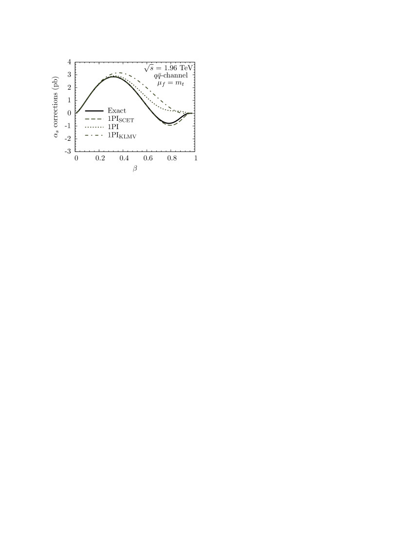
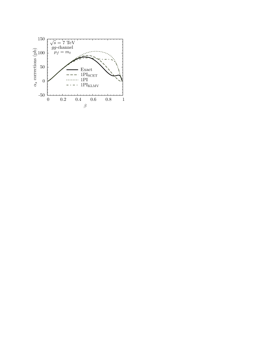
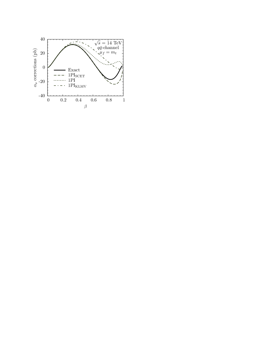
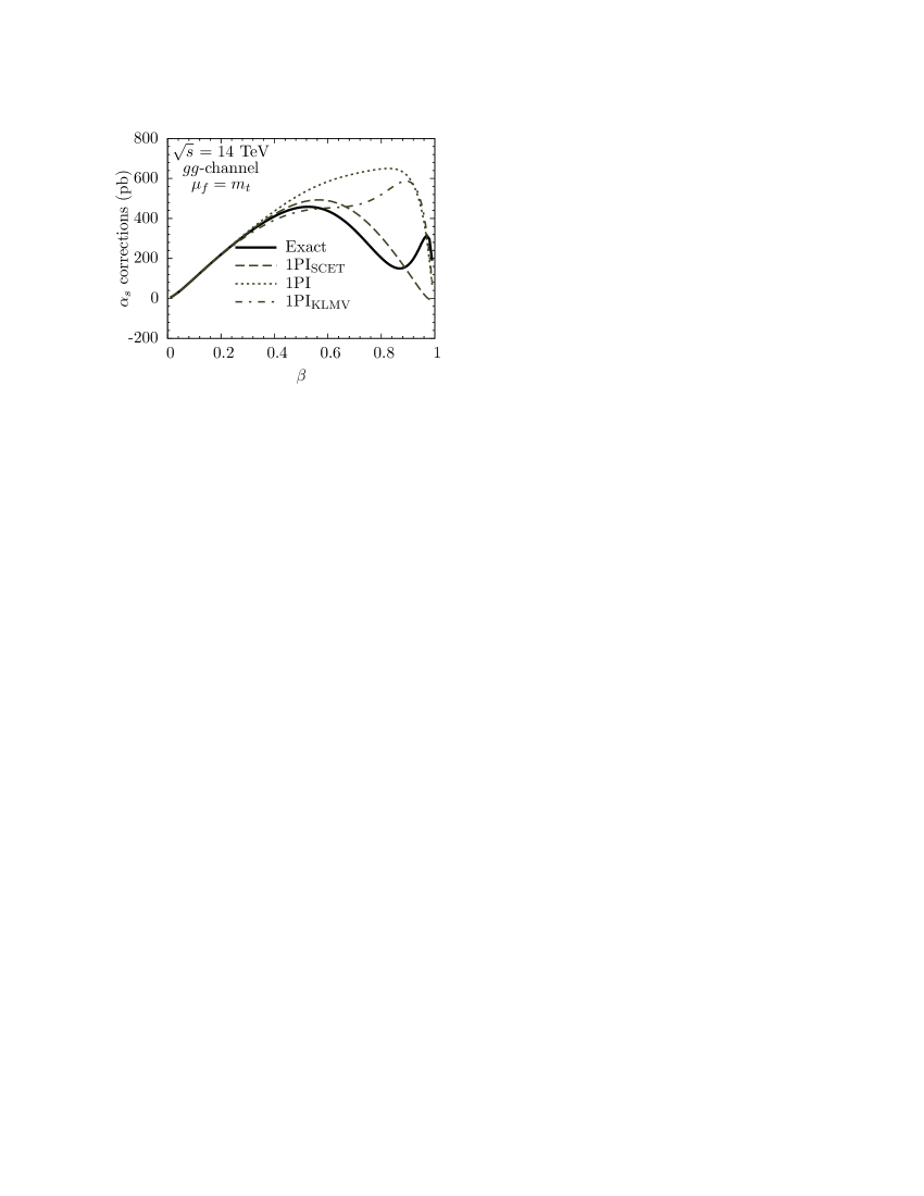
Figure 14: The $\alpha_{s}$ corrections to $d\sigma/d\beta$ for the choice $\mu_{f}=m_{t}$. The 1PI and $\text{1PI}_{\text{SCET}}$ results refer to the scheme used in the present work, while the 1PI_KLMV results uses that from [59].

Recently, approximate NNLO cross sections and $p_{T}$ distributions in 1PI kinematics have been calculated in [69]. While the resummation formalism leading to these results is different, we have checked wherever possible that the structure of the NNLO expansion as written in (39) is the same. Therefore, our results in the 1PI scheme (but not the $\text{1PI}_{\text{SCET}}$ scheme, which includes a set of corrections in the $R(s_{4})$ term in that equation), should in principle be the same. However, a direct comparison is complicated for two main reasons. First, no explicit analytic results for the coefficients appearing in (39) were given in [69], which focused instead on recalculating the two-loop anomalous dimension matrix obtained in [82, 83, 84]. As explained in the text after that equation, there are ambiguities in what terms to include in the coefficient multiplying the $\delta$-function term. Second, even if the scheme were fixed and the analytic expressions agreed, there would still be ambiguities in the numerical implementation, as explained in Section 4. In particular, depending on the choice of the variables $\hat{s}^{\prime}$, $\hat{t}_{1}^{\prime}$ and $\hat{u}_{1}^{\prime}$, the corrections stemming from the plus-distributions can be different. Since analytic results and the choice of scheme were not specified in [69], we cannot compare directly with the numerical results given there.

	Tevatron	LHC (7 TeV)	LHC (14 TeV)
$\sigma_{\rm NLO~{}leading,~{}1PI~{}(\text{1PI}_{\text{SCET}})}$	7.23${}^{+0.45}_{-0.86}$ (6.79${}^{+0.20}_{-0.70}$)	183${}^{+6}_{-18}$ (163${}^{+0}_{-11}$)	1024${}^{+0}_{-67}$ (887${}^{+0}_{-66}$)
$\sigma_{\rm NLO~{}leading,~{}PIM~{}(\text{PIM}_{\text{SCET}})}$	6.20${}^{+0.28}_{-0.69}$ (6.42${}^{+0.42}_{-0.76}$)	143${}^{+1}_{-12}$ (152${}^{+7}_{-15}$)	771${}^{+0}_{-42}$ (836${}^{+18}_{-60}$)
$\sigma_{\rm NNLO~{}approx,~{}1PI~{}(\text{1PI}_{\text{SCET}})}$	7.06${}^{+0.00}_{-0.29}$ (6.63${}^{+0.00}_{-0.27}$)	180${}^{+3}_{-8}$ (155${}^{+3}_{-2}$)	1009${}^{+40}_{-54}$ (851${}^{+25}_{-5}$)
$\sigma_{\rm NNLO~{}approx,~{}PIM~{}(\text{PIM}_{\text{SCET}})}$	6.46${}^{+0.18}_{-0.45}$ (6.62${}^{+0.05}_{-0.40}$)	148${}^{+14}_{-11}$ (155${}^{+8}_{-8}$)	823${}^{+78}_{-67}$ (860${}^{+46}_{-43}$)

Table 6: The total cross section in pb in the 1PI and PIM schemes, where the subleading terms produced through the SCET expansion are not included. The uncertainties are estimated from scale variation in the range $m_{t}/2<\mu_{f}<2m_{t}$. The results in the $\text{1PI}_{\text{SCET}}$ and $\text{PIM}_{\text{SCET}}$ schemes (also shown in Table 5) are listed in parentheses for comparison.

Instead, we shall present our own results in the 1PI and PIM schemes, and use those to compare with the $\text{1PI}_{\text{SCET}}$ and $\text{PIM}_{\text{SCET}}$ results. For the default scale choice $\mu_{f}=m_{t}=173.1$ GeV, the numbers in these schemes are shown in Table 6. Comparing with Table 5, we notice that the numbers in the $\text{PIM}_{\text{SCET}}$ and PIM schemes are in much better agreement than those in the $\text{1PI}_{\text{SCET}}$ and 1PI schemes. Actually, the $\text{PIM}_{\text{SCET}}$, $\text{1PI}_{\text{SCET}}$, and PIM results are compatible with each other within the uncertainties estimated through scale variations, while the 1PI results are much higher, especially at the LHC. Since all of our numerical studies have indicated that predictions in 1PI kinematics at LHC energies are susceptible to large power corrections, we are rather hesitant to give much weight to those particular results. We consider the results in PIM kinematics more reliable, and if different kinematics is to be used as a criterion for estimating uncertainties, we believe the situation is more accurately reflected in Tables 5 and 5 than in Table 6.

The approximate NNLO numbers in Table 6 are very close to those of [69] for the Tevatron, but at the LHC they are roughly 10% higher than those in [69]. While we are unable to pinpoint the source of this discrepancy for the reasons explained above, we can compare the leading singular terms in our 1PI expansion at NLO with those obtained in [59]. As explained in Section 4, these were obtained using a different scheme to evaluate the equivalent analytic results at threshold, so the difference between two numbers gives a rough measure of the power-suppressed ambiguities inherent to the formulas at threshold. In Figure 14 we compare the results of [59] with those obtained in our 1PI scheme, in the $\text{1PI}_{\text{SCET}}$ scheme, and with the exact results. As seen from the figure, the leading terms in the $\text{1PI}_{\text{SCET}}$ scheme provide the best approximation to the full results, and differences due to the choice of scheme get larger as the collider energy increases. The numbers in our 1PI scheme are higher than those from [59], which may account for the discrepancy with [69]. For reference, the leading singular terms at NLO with $\mu_{f}=m_{t}$ in the scheme of [59] yield cross sections of $7.42$ pb at the Tevatron, $174$ pb at the LHC with $\sqrt{s}=7$ TeV, and $968$ pb at the LHC with $\sqrt{s}=14$ TeV. In [69], it was stated that in the $gg$ channel the leading singular terms in 1PI kinematics account for over 98% of the NLO correction at both the Tevatron and the LHC. For this NLO correction, the exact results at $\mu_{f}=m_{t}$ are $0.42$ pb at the Tevatron and $280$ pb at the LHC with $\sqrt{s}=14$ TeV, compared to $0.44$ pb and $360$ pb for the leading singular pieces in the 1PI scheme of [59]. The number at the LHC is quite a bit higher than the exact result, and we therefore are not able to confirm the statement made in [69], although we cannot rule out that they were obtained in yet another (unspecified) scheme for evaluating the formulas at threshold.

7 Conclusions

We have used techniques from SCET to study higher-order perturbative corrections to 1PI observables in top-quark pair production at hadron colliders. In particular, we have calculated and collected the perturbative ingredients needed for an analysis at NLO+NNLL and approximate NNLO, and applied them to transverse-momentum and rapidity distributions as well as the total production cross sections at the Tevatron and LHC, and to the forward-backward asymmetry at the Tevatron. The details of factorization and resummation within our approach were mainly taken over from the analogous study in PIM kinematics presented in [55]. However, differences arise from the phase-space integrations for real emission in the soft limit. They affect the matrix-valued soft matching function, which must be calculated from scratch. We presented results for this matching function at NLO in fixed-order perturbation theory, which were previously unknown, and also addressed the differences in its RG equation needed for the resummation of soft gluon corrections to all orders. Along with the anomalous dimensions and matrix-valued hard matching functions already known from [55], these are the essential ingredients for an NLO+NNLL calculation.

Even apart from the new perturbative information included in our results, an important aspect of the SCET approach to threshold resummation is its ability to include a class of logarithmic corrections, which are formally subleading in the exact threshold limit but nonetheless give non-negligible numerical contributions. These arise in the SCET formalism by noticing that in a suitable reference frame the single dimensionful parameter characterizing soft radiation is the total soft energy $E_{s}$ of the emitted gluons, and expressing the logarithmic corrections in terms of $\ln(E_{s}/\mu)$, without further expansion. The subleading terms generated in this way are of the form $\ln(1+s_{4}/m_{t}^{2})/s_{4}$ in 1PI kinematics, and $\ln z/(1-z)$ in PIM kinematics (with $z=M^{2}/\hat{s}$). We have implemented these new terms in our numerical analysis summarized below, where results including them are referred to as the $\text{1PI}_{\text{SCET}}$ and $\text{PIM}_{\text{SCET}}$ schemes. Results neglecting them are referred to as the 1PI and PIM schemes and should correspond with previous results at a given order in perturbation theory.

Our improved calculations of the hard-scattering kernels near threshold are a priori only important in regions of phase space where kinematic restrictions imply the partonic threshold limit $s_{4}\to 0$. However, the differential cross section in such regions is very small. Beyond that, the improved predictions are important if a dynamical threshold enhancement occurs, due to a sharp fall-off of the PDFs away from integration regions where $s_{4}\to 0$. In Section 5 we performed a very detailed discussion of the mechanism of threshold enhancement, and compared its effectiveness in 1PI and PIM kinematics at the level of differential distributions and the total cross section. The main finding was that the leading power corrections to the threshold limit in 1PI kinematics, which scale as $E_{s}/m_{t}\sim s_{4}/m_{t}^{2}$, are in general larger than the leading corrections in PIM kinematics, which scale as $E_{s}/M\sim(1-z)$. At the LHC with $\sqrt{s}=14$ TeV these corrections can become quite large. This makes us somewhat reserved about the utility of the threshold expansion in 1PI kinematics, especially at larger values of $p_{T}$. Including the extra subleading terms unique to the $\text{1PI}_{\text{SCET}}$ approximation seemed to account for the power corrections to a good degree of accuracy in the $q\bar{q}$ channel and also to some level in the $gg$ channel, at least in regions of phase space where the differential cross section is large. Since the top-quark pair production cross section at the Tevatron is dominated by the quark-antiquark channel, the predictions obtained in the $\text{1PI}_{\text{SCET}}$ scheme at the Tevatron center-of-mass energy are expected to provide a reliable approximation to the exact results. In all cases, but especially at the LHC with $\sqrt{s}=14$ TeV, the pure 1PI expansion gave larger corrections compared to any other approximation, and we are rather skeptical of any results obtained in that scheme. For the reasons mentioned above, we limited the phenomenological analysis to areas where the differential distributions are fairly large, or else to integrated quantities such as the forward-backward asymmetry and the total cross section. Our results for the rapidity and transverse-momentum distributions can be found in Figures 10 and 11. As expected, including the higher-order perturbative corrections in the form of NLO+NNLL or approximate NNLO predictions leads to a stabilization of the results under variations of the different perturbative scales. Our main results for the total cross section can be found in Tables 5 and 5. Although we consider the $\text{PIM}_{\text{SCET}}$ numbers more trustworthy, it is reassuring that the $\text{1PI}_{\text{SCET}}$ numbers are actually in very good agreement with them. This is not the case for the pure 1PI numbers, which come out significantly larger in all cases. If different types of kinematics is to be used as a source of uncertainty in predictions based on soft-gluon resummation, we believe the true results are more accurately reflected in Tables 5 and 5.

In Section 6.3 and the Appendix we analyzed in detail the origin of the numerical differences between NLO+NNLL and approximate NNLO calculations. The structure of the plus-distributions considered in the two approaches is different, since in the resummation approach plus-distributions and logarithms of scale ratios are formally of the same order. We showed why our choice of the soft and hard scales for the NLO+NNLL calculations is sound and how the resummed results are stable with respect to reasonable variations of these scales.

In conclusion, we obtained NLO+NNLL predictions for the top-pair transverse-momentum and rapidity distributions at hadron colliders. In the case of the transverse-momentum distribution at the Tevatron, the predictions presented here can be already compared with experimental measurements. By integrating the results for the differential distributions we obtained predictions for fully inclusive observables such as the forward-backward asymmetry and the total cross section. For the total cross section in particular, we analyzed the relations among the $\text{1PI}_{\text{SCET}}$ results obtained here, the $\text{PIM}_{\text{SCET}}$ results of [55], and the ones obtained with a different resummation approach [69]. All the evidence gathered shows that the SCET-based approach provides consistent and reliable results in both types of kinematics.

Appendix A Appendix

In our numerical analysis we considered two different ways of including higher-order perturbative corrections to the hard-scattering kernels: constructing approximate expansions to NNLO in fixed order, and all-orders resummmation to NNLL accuracy. We emphasized that for a fixed numerical value of $\mu_{s}$, the truncation of the NNLL series to NNLO in $\alpha_{s}$ contains a different structure of corrections than the approximate NNLO formula. Here we explain this statement in more detail, and show explicitly what types of higher-order corrections the master formula (3.2) resums. To do so, it is sufficient to ignore the matrix structure of the RG equations, and just consider hard and soft functions which are simple functions of their arguments. Then the treatment of the hard function is straightforward, and the complication for the soft function is its non-locality.

To explain the issue, it is simplest to start with the hard function. Ignoring its matrix structure and dependence on kinematic invariants, its RG equation is of the form

$$\mu\frac{d}{d\mu}\,H(L_{h},\alpha_{s}(\mu))=\left(2\Gamma_{\rm cusp}\ln\frac{M^{2}}{\mu^{2}}+2\gamma^{h}\right)H(L_{h},\alpha_{s}(\mu))\,,$$ (61)

where $L_{h}\equiv\ln(M^{2}/\mu^{2})$. The parameter $M$ is to be understood as a generic hard scale; in the specific case of 1PI kinematics, it would be $M=\sqrt{\hat{s}}$. The RG equation can be used to generate higher-order terms in the perturbative expansion of $H$. For instance, we can solve the equation as a fixed-order series in $\alpha_{s}$ using the ansatz

$$H(L_{h},\alpha_{s}(\mu))=\alpha_{s}^{2}(\mu)\left[h^{(0,0)}+\frac{\alpha_{s}(\mu)}{4\pi}\,\sum_{n=0}^{2}h^{(1,n)}L_{h}^{n}+\dots\right].$$ (62)

In terms of the lowest-order coefficient and the anomalous dimensions and $\beta$-function, whose expansions we define as

$$\Gamma_{\text{cusp}}(\alpha_{s}) =\Gamma_{0}\,\frac{\alpha_{s}}{4\pi}+\Gamma_{1}\left(\frac{\alpha_{s}}{4\pi}\right)^{2}+\Gamma_{2}\left(\frac{\alpha_{s}}{4\pi}\right)^{3}+\ldots\,,$$

$$\beta(\alpha_{s}) =-2\alpha_{s}\left[\beta_{0}\,\frac{\alpha_{s}}{4\pi}+\beta_{1}\left(\frac{\alpha_{s}}{4\pi}\right)^{2}+\beta_{2}\left(\frac{\alpha_{s}}{4\pi}\right)^{3}+\ldots\right],$$ (63)

and similarly for $\gamma^{h}$, the expansion coefficients at NLO can be constructed as

$$H(L_{h},\alpha_{s}(\mu))=\alpha_{s}^{2}(\mu)\left\{h^{(0,0)}+\frac{\alpha_{s}(\mu)}{4\pi}\left[-h^{(0,0)}\left(\frac{\Gamma_{0}}{2}L_{h}^{2}+(\gamma^{h}_{0}+2\beta_{0})L_{h}\right)+h^{(1,0)}\right]+\dots\right\}.$$ (64)

One can obviously generalize this to any order in $\alpha_{s}$ and calculate the coefficients of the logarithms at a given order in terms of the anomalous dimensions and lower-order matching coefficients. This is the method used in constructing approximate fixed-order expansions.

In the effective-theory analysis, one assumes the presence of a second, widely separated scale $\mu_{s}\ll M$ and uses the counting of RG-improved perturbation theory, i.e. $\ln(\mu_{s}/M)\sim 1/\alpha_{s}$. Then the higher-order corrections contain large logarithms, which can be resummed to all-orders by using the exact solution to the RG equation. This solution reads [85]

$$H(L_{h},\alpha_{s}(\mu))=e^{4S(\mu_{h},\mu)-2a_{\gamma^{h}}(\mu_{h},\mu)}\,H\bigg{(}\ln\frac{M^{2}}{\mu_{h}^{2}},\alpha_{s}(\mu_{h})\bigg{)}\left(\frac{M}{\mu_{h}}\right)^{-2\eta_{h}},$$ (65)

where $\eta_{h}=2a_{\Gamma}(\mu_{h},\mu)$. The Sudakov exponent and normal anomalous exponent are

$$S(\mu_{h},\mu)=-\int\limits_{\alpha_{s}(\mu_{h})}^{\alpha_{s}(\mu)}\!d\alpha\,\frac{\Gamma_{\text{cusp}}(\alpha)}{\beta(\alpha)}\int\limits_{\alpha_{s}(\mu_{h})}^{\alpha}\!\frac{d\alpha^{\prime}}{\beta(\alpha^{\prime})}\,,\qquad a_{\Gamma}(\mu_{h},\mu)=-\int\limits^{\alpha_{s}(\mu)}_{\alpha_{s}(\mu_{h})}\!d\alpha\,\frac{\Gamma_{\text{cusp}}(\alpha)}{\beta(\alpha)}\,,$$ (66)

and similarly for $a_{\gamma^{h}}$.

The all-orders solution does not actually depend on $\mu_{h}$, as indicated by the notation. The same is true if the matching coefficient and the exponentials are consistently re-expanded as a series in $\alpha_{s}(\mu)$ in fixed order, in which case one just gets back the approximate formulas above. In practice, however, one must truncate the result at a given level of accuracy (e.g. NNLL), and beyond that level a residual dependence on $\mu_{h}$ remains. To avoid large logarithms in the matching coefficients, one chooses $\mu_{h}\sim M$ and runs to the scale $\mu_{f}$ using the all-orders solution. Then the exponential factors resum logarithms which count as $\ln(M^{2}/\mu_{f}^{2})$ and are large for $\mu_{f}\sim\mu_{s}$. To see this explicitly, we get rid of $\alpha_{s}(\mu_{h})$ everywhere by using (with $a(\mu_{f})\equiv\alpha_{s}(\mu_{f})/4\pi$)

$$a(\mu_{h})=\frac{a(\mu_{f})}{X}-\frac{a(\mu_{f})^{2}}{X^{2}}\,\frac{\beta_{1}}{\beta_{0}}\,\ln X+\dots\,;\qquad X=1+\beta_{0}\,a(\mu_{f})\,\ln\frac{\mu_{h}^{2}}{\mu_{f}^{2}}\,,$$ (67)

and re-expand the solution in (65) as a series in $a(\mu_{f})$. For reference, the expansion of the Sudakov factor and anomalous exponent to NNLO read

$$S(\mu_{h},\mu_{f}) =-a(\mu_{f})\,\frac{\Gamma_{0}}{8}\,L_{hf}^{2}+a(\mu_{f})^{2}\left(\frac{\beta_{0}\Gamma_{0}}{24}L_{hf}^{3}-\frac{\Gamma_{1}}{8}L_{hf}^{2}\right)+\dots\,,$$ (68)

$$a_{\Gamma}(\mu_{h},\mu_{f}) =a(\mu_{f})\,\frac{\Gamma_{0}}{2}\,L_{hf}+a(\mu_{f})^{2}\left(-\frac{\beta_{0}\Gamma_{0}}{4}L_{hf}^{2}+\frac{\Gamma_{1}}{2}L_{hf}\right)+\dots\,,$$ (69)

where $L_{hf}\equiv\ln(\mu_{h}^{2}/\mu_{f}^{2})$. The expansion of $a_{\gamma}$ is identical to the one in (69), with the replacements $\Gamma_{i}\to\gamma_{i}$.

Using the above equations to expand (65) to NLO, one recovers the NLO solution (64). All the dependence on $\mu_{h}$ drops out to that order, as long as we keep the one-loop matching correction. However, this is not the case if we expand our NLL approximation of the resummed hard function to NLO. In that case, the NLO matching coefficient is of higher-order in the counting and not included in the formula, so after expansion to NLO dependence on the scale $\mu_{h}$ remains. The direct expansion of our NLL formula at NLO in fixed order reads

$$\alpha_{s}^{2}(\mu_{f})\,a(\mu_{f})\left\{-h^{(0,0)}\ln\frac{\mu_{h}^{2}}{\mu_{f}^{2}}\left[\frac{\Gamma_{0}}{2}\ln\frac{\mu_{h}^{2}}{\mu_{f}^{2}}+\Gamma_{0}\ln\frac{M^{2}}{\mu_{h}^{2}}+(\gamma^{h}_{0}+2\beta_{0})\right]\right\}.$$ (70)

This is necessarily different than the “approximate NLO” formula one would deduce by dropping the coefficient $h^{(1,0)}$ from (64), because it depends on $\mu_{h}$, but if we set $\mu_{h}=M$ it is the same, and it is for this reason that one can still say the NLL solution “resums logarithms of the form $\ln(M/\mu_{f})$ to all orders”, although a more accurate statement would be that it “resums logarithms of the form $\ln(\mu_{h}/\mu_{f})$ to all orders”, which includes the possibility of other choices such as $\mu_{h}=m_{t}$. Given this fact, it makes little sense to construct an approximate formula for a quantity such as the hard function: if there are large logarithms, it is just as easy to sum them to all orders as it is to construct the fixed-order expansion, and if the logarithms are not large, there is no reason to include that subset of the higher-order corrections without the full answer.

We can repeat the analysis above to compare the structure of approximate fixed-order expansions and resummed formulas for the soft function. In this case the RG equation is non-local, and to solve for the momentum-space soft function one uses the technique of Laplace transforms [71]. The solution for the resummed momentum-space soft function is

$$S(\omega,\mu_{f})=e^{-4S(\mu_{s},\mu_{f})+2a_{\gamma^{s}}(\mu_{s},\mu_{f})}\,\tilde{s}\left(\partial_{\eta},\mu_{s}\right)\frac{1}{\omega}\left(\frac{\omega}{\mu_{s}}\right)^{2\eta}\frac{e^{-2\gamma_{E}\eta}}{\Gamma(2\eta)}\,,$$ (71)

where $\eta=2a_{\Gamma}(\mu_{s},\mu_{f})$, and $\tilde{s}$ is the Laplace-transformed function, which satisfies the local RG equation

$$\frac{d}{d\ln\mu}\,\tilde{s}\bigg{(}\ln\frac{M^{2}}{\mu^{2}},\alpha_{s}(\mu)\bigg{)}=-\left(2\Gamma_{\rm cusp}\ln\frac{M^{2}}{\mu^{2}}+2\gamma_{s}\right)\tilde{s}\bigg{(}\ln\frac{M^{2}}{\mu^{2}},\alpha_{s}(\mu)\bigg{)}\,.$$ (72)

In this case, approximate formulas in fixed order are obtained by first constructing the solution to $\tilde{s}$ using the local RG equation. To NNLO, we use the ansatz

$$\tilde{s}(L,\alpha_{s}(\mu))=1+\frac{\alpha_{s}(\mu)}{4\pi}\,\sum_{n=0}^{2}s^{(1,n)}L^{n}+\left(\frac{\alpha_{s}(\mu)}{4\pi}\right)^{2}\sum_{n=0}^{4}s^{(2,n)}L^{n}+\dots\,,$$ (73)

where we set $s^{(0,0)}=1$ for simplicity. The explicit solution to NNLO reads

$$\tilde{s}(L,\alpha_{s}(\mu)) =1+\frac{\alpha_{s}(\mu)}{4\pi}\left[\frac{\Gamma_{0}}{2}L^{2}+L\gamma^{s}_{0}+s^{(1,0)}\right]$$

$$+\left(\frac{\alpha_{s}(\mu)}{4\pi}\right)^{2}\bigg{[}\frac{\Gamma_{0}^{2}}{8}L^{4}+\left(-\frac{\beta_{0}\Gamma_{0}}{6}+\frac{\Gamma_{0}\gamma^{s}_{0}}{2}\right)L^{3}+\frac{1}{2}\left(\Gamma_{1}-\beta_{0}\gamma^{s}_{0}+(\gamma^{s}_{0})^{2}+\Gamma_{0}s^{(1,0)}\right)L^{2}$$

$$\hskip 73.97733pt+(\gamma^{s}_{1}-\beta_{0}s^{(1,0)}+\gamma^{s}_{0}s^{(1,0)})L+s^{(2,0)}\bigg{]}.$$ (74)

To turn this into an approximate NNLO formula for the momentum-space soft function $S(\omega,\mu_{f})$, one must take the limit $\mu_{s}=\mu_{f}$ and derive replacement rules analogous to (38). This is readily done using the expansion

$$\frac{1}{\omega}\left(\frac{\omega}{\mu_{s}}\right)^{2\eta}=\frac{1}{2\eta}\,\delta(\omega)+\sum_{n=0}^{\infty}\frac{2^{n}}{n!}\,D_{n}(\omega)\,\eta^{n}\,,$$ (75)

where the $D_{n}$ are defined as

$$D_{n}(\omega)=\left[\frac{1}{\omega}\,\ln^{n}\frac{\omega}{\mu_{f}}\right]_{+}.$$ (76)

As was the case with the hard function, the all-orders solution for the resummed soft function does not actually depend on the scale $\mu_{s}$, but its truncation to a given logarithmic order (e.g. NNLL) introduces residual scale dependence. As explained earlier in the paper, our method is to choose $\mu_{s}$ to be close to the numerical value where the corrections from the soft function to the (differential) cross section are minimal. We then adopt the parametric counting $\mu_{s}\sim\omega$ and apply RG-improved perturbation theory with $\ln\mu_{s}/\mu_{f}\sim 1/\alpha_{s}$, and the exponential factors resum logarithms of the form $\ln\mu_{s}/\mu_{f}$ to all orders. Since the scale $\mu_{s}$ is dynamically generated through the numerical analysis, it does not appear in the fixed-order calculation, so the resummation formula deals with different types of corrections than the approximate fixed-order formulas. For this reason, the structure of $D_{n}$ distributions appearing at a given order is not the same in the two approaches.

We now show this in more detail, working first to NLO. In this case, the “approximate NLO” formula derived from the solution (A) reads

$$S(\omega,\mu_{f})\approx 1+a(\mu_{f})\left[4\Gamma_{0}D_{1}(\omega)+2\gamma^{s}_{0}D_{0}(\omega)-\frac{\pi^{2}}{3}\Gamma_{0}\,\delta(\omega)\right].$$ (77)

This should be compared with the expansion of the NLL formula to NLO in fixed order, for which the NLO correction reads (with $L_{s}\equiv\ln\mu_{s}^{2}/\mu_{f}^{2}$)

$$a(\mu_{f})\left[2\Gamma_{0}L_{s}D_{0}(\omega)+\left(\frac{1}{2}\Gamma_{0}L_{s}^{2}+\gamma_{0}^{s}L_{s}\right)\delta(\omega)\right]+\dots\,.$$ (78)

The “approximate NLO” formula has $D_{1}$ distributions, while the NLO expansion of our NLL formula has only $D_{0}$ distributions. In the counting of RG-improved perturbation theory, however, $D_{0}\ln(\mu_{s}/\mu_{f})\sim D_{1}$, so the tower of logarithms produced by the expansion of the NLL formulas is of course correct. The analogous formula at NNLO is rather lengthy, but to illustrate its structure, we focus on the leading correction in the logarithmic power counting, which reads

$$a(\mu_{f})^{2}\Gamma_{0}^{2}\left[12L_{s}D_{2}(\omega)-6L_{s}^{2}D_{1}(\omega)+L_{s}^{3}D_{0}-\frac{1}{8}L_{s}^{4}\,\delta(\omega)\right],$$ (79)

while the leading term of the “approximate NNLO” formula is

$$a(\mu_{f})^{2}\,8\Gamma_{0}^{2}\,D_{3}(\omega)\,.$$ (80)

Again, for $\omega\sim\mu_{s}$ the terms in the two equations are of the same parameteric order but contain different types of distributions: the resummed formulas generate at most $D_{2}$ distributions, while the approximate NNLO formulas generate $D_{3}$ distributions.

From the discussion above it should be obvious that our formula does not literally resum the highest tower of $D_{n}$ distributions to all orders, but rather terms which count that way in RG-improved perturbation theory, when the dynamically generated soft scale satisfies $\mu_{s}\sim\omega$. In the case of the hard function, we noted that the fixed-order corrections produced by expanding the resummed formula were equal to those in the approximate formula for the special choice $\mu_{h}=M$. For the soft function, there is no numerical value of $\mu_{s}$ for which this would be true, but the two are equal if we replace $L_{s}\to\partial_{\eta}$ and take the derivatives before re-expanding $\eta$ in $\alpha_{s}(\mu_{f})$. This procedure can be generalized to all orders by evaluating the formula

$$S(\omega,\mu_{f})=\left\{\left[e^{-4S(\mu_{s},\mu_{f})+2a_{\gamma^{s}}(\mu_{s},\mu_{f})}\tilde{s}\left(0,\alpha_{s}(\mu_{s})\right)\right]\bigg{|}_{\ln(\mu_{s}^{2}/\mu_{f}^{2})\to\partial\eta}\right\}\frac{1}{\omega}\left(\frac{\omega}{\mu_{f}}\right)^{2\eta}\frac{e^{-2\gamma_{E}\eta}}{\Gamma(2\eta)}\bigg{|}_{\eta\to 0}\,,$$ (81)

where the factor in the curly brackets is understood to be expanded to all orders as a series in $\alpha_{s}(\mu_{f})$ and so is a function only of $\ln(\mu_{s}^{2}/\mu_{f}^{2})$. In this way, we exponentiate the derivatives with respect to $\eta$, which are what generate the highest-order distributions, and the expansion of the above formula to any given accuracy in fixed-order reproduces the approximate formulas. For instance, if we include the exact one-loop matching (which is just $s^{(1,0)}$) and the two-loop anomalous dimensions, the expansion of the above object gives back our approximate NNLO formula for the soft function, plus higher-order terms that resum all the higher-order $D_{n}$ distributions at NNLL order, after converting the derivatives with respect to $\eta$ with replacement rules. While this procedure generalizes choosing $\mu_{h}=M$ in the hard function, it is by no means the same conceptually. The exact hard function is independent of $\mu_{h}$, so varying it around values $\mu_{h}\sim M$ gives a way of estimating the higher-order terms. However, it would make no sense to replace, for instance, $\ln(\mu_{s}^{2}/\mu_{f}^{2})\to c_{0}\partial_{\eta}$ in (81), with $c_{0}\neq 1$, since the derivatives generate both $\mu$-independent and $\mu$-dependent terms.

The conclusion of this discussion is that results based on approximate NNLO formulas contain different information than those based on NLO+NNLL resummation. This is not just due to a truncation of the NNLL series to NNLO, but also to the fact that the resummation formula exponentiates logarithms depending on the ratio $\ln\mu_{s}/\mu_{f}$ in combination with higher-order logarithmic plus-distributions, with $\mu_{s}$ a dynamically generated numerical soft scale. Such logarithms do not appear in the fixed-order calculation, which is independent of $\mu_{s}$. Therefore, the choice between using approximate NNLO and NLO+NNLL amounts to whether one takes seriously the improved convergence of the soft function at a numerically small soft scale. If so, one should use the resummed formulas, if not, one should use the approximate fixed-order calculations. In practice, this question can only be answered after a numerical analysis, and for this reason, we have evaluated both types of formulas in the studies in Sections 5 and 6.

References

- [1] CDF and D0 Collaboration, arXiv:1007.3178 [hep-ex].
- [2] H. Flächer, M. Goebel, J. Haller, A. Hocker, K. Monig and J. Stelzer, Eur. Phys. J. C 60, 543 (2009) [arXiv:0811.0009 [hep-ph]].
- [3] R. Frederix and F. Maltoni, JHEP 0901, 047 (2009) [arXiv:0712.2355 [hep-ph]].
- [4] V. Barger, T. Han and D. G. E. Walker, Phys. Rev. Lett. 100, 031801 (2008) [arXiv:hep-ph/0612016].
- [5] U. Baur and L. H. Orr, Phys. Rev. D 77, 114001 (2008) [arXiv:0803.1160 [hep-ph]].
- [6] C. T. Hill and S. J. Parke, Phys. Rev. D 49, 4454 (1994) [arXiv:hep-ph/9312324].
- [7] T. Aaltonen et al. [CDF Collaboration], Phys. Rev. Lett. 101, 202001 (2008) [arXiv:0806.2472 [hep-ex]].
- [8] V. M. Abazov et al. [D0 Collaboration], Phys. Rev. Lett. 100, 142002 (2008) [arXiv:0712.0851 [hep-ex]].
- [9] T. Aaltonen et al. [CDF Collaboration], arXiv:1101.0034 [hep-ex].
- [10] F. Abe et al. [CDF Collaboration], Phys. Rev. Lett. 74, 2626 (1995) [arXiv:hep-ex/9503002].
- [11] V. Khachatryan et al. [CMS Collaboration], Phys. Lett. B 695, 424 (2011) [arXiv:1010.5994 [hep-ex]].
- [12] G. Aad et al. [ATLAS Collaboration], arXiv:1012.1792 [hep-ex].
- [13] W. Bernreuther, arXiv:1008.3819 [hep-ph].
- [14] W. Bernreuther, J. Phys. G 35, 083001 (2008) [arXiv:0805.1333 [hep-ph]].
- [15] P. Nason, S. Dawson and R. K. Ellis, Nucl. Phys. B 303, 607 (1988).
- [16] W. Beenakker, H. Kuijf, W. L. van Neerven and J. Smith, Phys. Rev. D 40, 54 (1989).
- [17] W. Beenakker, W. L. van Neerven, R. Meng, G. A. Schuler and J. Smith, Nucl. Phys. B 351, 507 (1991).
- [18] M. Czakon and A. Mitov, Nucl. Phys. B 824, 111 (2010) [arXiv:0811.4119 [hep-ph]].
- [19] P. Nason, S. Dawson and R. K. Ellis, Nucl. Phys. B 327, 49 (1989) [Erratum-ibid. B 335, 260 (1990)].
- [20] M. L. Mangano, P. Nason and G. Ridolfi, Nucl. Phys. B 373, 295 (1992).
- [21] S. Frixione, M. L. Mangano, P. Nason and G. Ridolfi, Phys. Lett. B 351, 555 (1995) [arXiv:hep-ph/9503213].
- [22] J. H. Kühn and G. Rodrigo, Phys. Rev. Lett. 81, 49 (1998) [arXiv:hep-ph/9802268].
- [23] J. H. Kühn and G. Rodrigo, Phys. Rev. D 59, 054017 (1999) [arXiv:hep-ph/9807420].
- [24] M. Czakon, A. Mitov and S. Moch, Phys. Lett. B 651, 147 (2007) [arXiv:0705.1975 [hep-ph]].
- [25] M. Czakon, A. Mitov and S. Moch, Nucl. Phys. B 798, 210 (2008) [arXiv:0707.4139 [hep-ph]].
- [26] M. Czakon, Phys. Lett. B 664, 307 (2008) [arXiv:0803.1400 [hep-ph]].
- [27] R. Bonciani, A. Ferroglia, T. Gehrmann, D. Maitre and C. Studerus, JHEP 0807, 129 (2008) [arXiv:0806.2301 [hep-ph]].
- [28] R. Bonciani, A. Ferroglia, T. Gehrmann and C. Studerus, JHEP 0908, 067 (2009) [arXiv:0906.3671 [hep-ph]].
- [29] R. Bonciani, A. Ferroglia, T. Gehrmann, A. Manteuffel and C. Studerus, JHEP 1101, 102 (2011) [arXiv:1011.6661 [hep-ph]].
- [30] J. G. Korner, Z. Merebashvili and M. Rogal, Phys. Rev. D 77, 094011 (2008) [arXiv:0802.0106 [hep-ph]].
- [31] C. Anastasiou and S. M. Aybat, Phys. Rev. D 78, 114006 (2008) [arXiv:0809.1355 [hep-ph]].
- [32] B. Kniehl, Z. Merebashvili, J. G. Korner and M. Rogal, Phys. Rev. D 78, 094013 (2008) [arXiv:0809.3980 [hep-ph]].
- [33] S. Dittmaier, P. Uwer and S. Weinzierl, Phys. Rev. Lett. 98, 262002 (2007) [arXiv:hep-ph/0703120].
- [34] S. Dittmaier, P. Uwer and S. Weinzierl, Nucl. Phys. Proc. Suppl. 183, 196 (2008) [arXiv:0807.1223 [hep-ph]].
- [35] G. Bevilacqua, M. Czakon, C. G. Papadopoulos and M. Worek, Phys. Rev. Lett. 104, 162002 (2010) [arXiv:1002.4009 [hep-ph]].
- [36] K. Melnikov and M. Schulze, Nucl. Phys. B 840, 129 (2010) [arXiv:1004.3284 [hep-ph]].
- [37] M. Czakon, Phys. Lett. B 693, 259 (2010) [arXiv:1005.0274 [hep-ph]].
- [38] M. Czakon, arXiv:1101.0642 [hep-ph].
- [39] G. Sterman, Nucl. Phys. B 281, 310 (1987).
- [40] S. Catani and L. Trentadue, Nucl. Phys. B 327, 323 (1989).
- [41] E. Laenen, J. Smith and W. L. van Neerven, Nucl. Phys. B 369, 543 (1992).
- [42] E. Laenen, J. Smith and W. L. van Neerven, Phys. Lett. B 321, 254 (1994) [arXiv:hep-ph/9310233].
- [43] E. L. Berger and H. Contopanagos, Phys. Lett. B 361, 115 (1995) [arXiv:hep-ph/9507363].
- [44] E. L. Berger and H. Contopanagos, Phys. Rev. D 54, 3085 (1996) [arXiv:hep-ph/9603326].
- [45] E. L. Berger and H. Contopanagos, Phys. Rev. D 57, 253 (1998) [arXiv:hep-ph/9706206].
- [46] S. Catani, M. L. Mangano, P. Nason and L. Trentadue, Phys. Lett. B 378, 329 (1996) [arXiv:hep-ph/9602208].
- [47] R. Bonciani, S. Catani, M. L. Mangano and P. Nason, Nucl. Phys. B 529, 424 (1998) [Erratum-ibid. B 803, 234 (2008)] [arXiv:hep-ph/9801375].
- [48] S. Moch and P. Uwer, Phys. Rev. D 78, 034003 (2008) [arXiv:0804.1476 [hep-ph]].
- [49] M. Czakon and A. Mitov, Phys. Lett. B 680, 154 (2009) [arXiv:0812.0353 [hep-ph]].
- [50] U. Langenfeld, S. Moch and P. Uwer, Phys. Rev. D 80, 054009 (2009) [arXiv:0906.5273 [hep-ph]].
- [51] M. Beneke, P. Falgari and C. Schwinn, Nucl. Phys. B 828, 69 (2010) [arXiv:0907.1443 [hep-ph]].
- [52] M. Czakon, A. Mitov and G. Sterman, Phys. Rev. D 80, 074017 (2009) [arXiv:0907.1790 [hep-ph]].
- [53] M. Beneke, M. Czakon, P. Falgari, A. Mitov and C. Schwinn, Phys. Lett. B 690, 483 (2010) [arXiv:0911.5166 [hep-ph]].
- [54] M. Beneke, P. Falgari and C. Schwinn, Nucl. Phys. B 842, 414 (2011) [arXiv:1007.5414 [hep-ph]].
- [55] V. Ahrens, A. Ferroglia, M. Neubert, B. D. Pecjak and L. L. Yang, JHEP 1009, 097 (2010) [arXiv:1003.5827 [hep-ph]].
- [56] N. Kidonakis and G. Sterman, Phys. Lett. B 387, 867 (1996).
- [57] N. Kidonakis and G. Sterman, Nucl. Phys. B 505, 321 (1997) [arXiv:hep-ph/9705234].
- [58] N. Kidonakis, Phys. Rev. D 64, 014009 (2001) [arXiv:hep-ph/0010002].
- [59] N. Kidonakis, E. Laenen, S. Moch and R. Vogt, Phys. Rev. D 64, 114001 (2001) [arXiv:hep-ph/0105041].
- [60] N. Kidonakis and R. Vogt, Phys. Rev. D 68, 114014 (2003) [arXiv:hep-ph/0308222].
- [61] A. Banfi and E. Laenen, Phys. Rev. D 71, 034003 (2005) [arXiv:hep-ph/0411241].
- [62] L. G. Almeida, G. Sterman and W. Vogelsang, Phys. Rev. D 78, 014008 (2008) [arXiv:0805.1885 [hep-ph]].
- [63] N. Kidonakis and R. Vogt, Phys. Rev. D 78, 074005 (2008) [arXiv:0805.3844 [hep-ph]].
- [64] V. Ahrens, A. Ferroglia, M. Neubert, B. D. Pecjak and L. L. Yang, Phys. Lett. B 687, 331 (2010) [arXiv:0912.3375 [hep-ph]].
- [65] T. Becher, M. Neubert and G. Xu, JHEP 0807, 030 (2008) [arXiv:0710.0680 [hep-ph]].
- [66] V. Ahrens, T. Becher, M. Neubert and L. L. Yang, Phys. Rev. D 79, 033013 (2009) [arXiv:0808.3008 [hep-ph]].
- [67] V. Ahrens, T. Becher, M. Neubert and L. L. Yang, Eur. Phys. J. C 62, 333 (2009) [arXiv:0809.4283 [hep-ph]].
- [68] E. Laenen, G. Oderda and G. Sterman, Phys. Lett. B 438, 173 (1998) [arXiv:hep-ph/9806467].
- [69] N. Kidonakis, Phys. Rev. D 82, 114030 (2010) [arXiv:1009.4935 [hep-ph]].
- [70] S. Fleming, A. H. Hoang, S. Mantry and I. W. Stewart, Phys. Rev. D 77, 074010 (2008) [arXiv:hep-ph/0703207].
- [71] T. Becher and M. Neubert, Phys. Rev. Lett. 97, 082001 (2006) [arXiv:hep-ph/0605050].
- [72] T. Becher, M. Neubert and B. D. Pecjak, JHEP 0701, 076 (2007) [arXiv:hep-ph/0607228].
- [73] C. W. Bauer, N. D. Dunn and A. Hornig, arXiv:1010.0243 [hep-ph].
- [74] A. D. Martin, W. J. Stirling, R. S. Thorne and G. Watt, Eur. Phys. J. C 64, 653 (2009) [arXiv:0905.3531 [hep-ph]].
- [75] H. L. Lai, J. Huston, Z. Li, P. Nadolsky, J. Pumplin, D. Stump and C. P. Yuan, Phys. Rev. D 82, 054021 (2010) [arXiv:1004.4624 [hep-ph]].
- [76] J. M. Campbell and R. K. Ellis, Phys. Rev. D 62, 114012 (2000) [arXiv:hep-ph/0006304].
- [77] J. Alwall et al., JHEP 0709, 028 (2007) [arXiv:0706.2334 [hep-ph]].
- [78] R. Frederix, S. Frixione, F. Maltoni and T. Stelzer, JHEP 0910, 003 (2009) [arXiv:0908.4272 [hep-ph]].
- [79] V. M. Abazov et al. [D0 Collaboration], Phys. Lett. B 693, 515 (2010) [arXiv:1001.1900 [hep-ex]].
- [80] V. Ahrens, A. Ferroglia, M. Neubert, B. D. Pecjak and L. L. Yang, in preparation.
- [81] V. M. Abazov et al. [D0 Collaboration], Phys. Rev. D 80, 071102 (2009) [arXiv:0903.5525 [hep-ex]].
- [82] T. Becher and M. Neubert, Phys. Rev. D 79, 125004 (2009) [Erratum-ibid. D 80, 109901 (2009)] [arXiv:0904.1021 [hep-ph]].
- [83] A. Ferroglia, M. Neubert, B. D. Pecjak and L. L. Yang, Phys. Rev. Lett. 103, 201601 (2009) [arXiv:0907.4791 [hep-ph]].
- [84] A. Ferroglia, M. Neubert, B. D. Pecjak and L. L. Yang, JHEP 0911, 062 (2009) [arXiv:0908.3676 [hep-ph]].
- [85] S. W. Bosch, R. J. Hill, B. O. Lange and M. Neubert, Phys. Rev. D 67, 094014 (2003) [arXiv:hep-ph/0301123].