Investigating a model of optimised AGN feedback

Abstract

Feedback heating from AGN in massive galaxies and galaxy clusters can be thought of as a naturally occurring control system which plays a significant role in regulating both star formation rates and the X-ray luminosity of the surrounding hot gas. In the simplest case, negative feedback can be viewed as a system response that is ‘optimised’ to minimise deviations from equilibrium, such that the system rapidly evolves towards a steady state. However, a general solution of this form appears to be incompatible with radio observations which indicate intermittent AGN outbursts. Here, we explore an energetically favourable scenario in which feedback is required to both balance X-ray gas cooling, and minimise the sum of the energy radiated by the gas and the energy injected by the AGN. This specification is equivalent to ensuring that AGN heating balances the X-ray gas cooling with minimum black hole growth. It is shown that minimum energy heating occurs in discrete events, and not at a continuous, constant level. Furthermore, systems with stronger feedback experience proportionally more powerful heating events, but correspondingly smaller duty cycles. Interpreting observations from this perspective would imply that stronger feedback occurs in less massive objects - elliptical galaxies, rather than galaxy clusters. One direct consequence of this effect would be that AGN heating events are sufficiently powerful to expel hot gas from the gravitational potential of a galaxy, but not a galaxy cluster, which is consistent with theoretical explanations for the steepening of the $L_{\rm X}-T$ relation at temperatures below 1-2 keV.

1 Introduction

The cooling time of X-ray emitting gas in the cores of many massive galaxies and galaxy clusters is much shorter than the Hubble time. In the absence of heat sources, the gas will cool and form stars. However, high-resolution X-ray spectroscopy of galaxies and clusters has shown that the rate at which gas cools to low temperatures is significantly reduced compared to preliminary expectations (e.g. Peterson et al., 2001; Tamura et al., 2001; Xu et al., 2002; Sakelliou et al., 2002; Peterson et al., 2003; Kaastra et al., 2004; Peterson & Fabian, 2006) suggesting that the gas is somehow being reheated.

Numerous possible heating mechanisms have been suggested, most notably energy injection by Active Galactic Nuclei (AGN) (e.g. Binney & Tabor, 1995; Tucker & David, 1997; Ciotti & Ostriker, 2001) and the inward flux of thermal energy from large radii due to thermal conduction (e.g. Bregman & David, 1988; Gaetz, 1989; Zakamska & Narayan, 2003; Pope et al., 2005). Quantifying these heating processes is difficult due our incomplete understanding of the microphysics of the X-ray emitting plasma (see Cho et al., 2003; Parrish et al., 2009, for example). Nevertheless, due to its strong temperature dependence, thermal conduction alone probably cannot provide a general solution to the cooling flow problem (e.g. Voigt & Fabian, 2004; Pope et al., 2006; Guo et al., 2008).

Instead, it is generally assumed that energy input by a central AGN is predominantly responsible for reheating the gas. This is partly based on a wealth of observational evidence which indicates that radio AGN outflows are triggered in response to the thermal state of their environment (e.g. Burns, 1990; Best et al., 2005; Bîrzan et al., 2004; Dunn et al., 2005; Best, 2007; Rafferty et al., 2008; Cavagnolo et al., 2008; Mittal et al., 2009). If true, this suggests that AGN activity is part of a negative feedback loop which may regulate properties of its environment.

Theoretical studies have also provided complimentary evidence highlighting the importance of AGN feedback. For example, implementations of AGN heating in semi-analytic models of galaxy formation have shown that, in principle, AGN can both reheat cooling flows and explain the exponential cutoff at the bright end of the galaxy luminosity function (e.g. Benson et al., 2003; Croton et al., 2006; Bower et al., 2006; Short & Thomas, 2009). More recently, AGN heating has been shown to be fundamental in shaping the X-ray luminosity-temperature of massive galaxies (e.g. Puchwein et al., 2008; Bower et al., 2008; Pope, 2009).

Broadly speaking, theoretical studies employ AGN heating as an input with which to control star formation rates and the X-ray luminosity of the hot gas that permeates massive galaxies and galaxy clusters. Essentially, this conceptualises AGN feedback as a control system similar to a thermostat (c.f. Kaiser, 2007). This approach can be highly informative; AGN feedback is an extremely complex phenomenon which depends on poorly understood physical processes occurring across a huge range of spatial scales. As yet, numerical hydrodynamic simulations do not include sufficient physical processes to naturally reproduce observations without being complemented by additional numerical prescriptions. Yet, even if the simulations were physically complete, the outcomes would still need to be interpreted.

For this reason, we investigate AGN feedback in the most general way, by expressing its overall effect in terms of well-defined global quantities, and comparing the main results with observations. For example, consider the simplest case, in which AGN heating is regulated only by negative feedback. Negative feedback can be defined as a response which occurs to oppose its cause. Therefore, unless forced to do otherwise, it will tend to minimise deviations from some equilibrium condition. Thus, in general, a system regulated purely by negative feedback will rapidly tend towards a steady state in which the controller is permanently active at a constant value. Notably, this does not appear to be the case for AGN feedback, and it is imperative to note that minimising deviations from an equilibrium state is only one measure of the performance of feedback. Depending on additional constraints it can also be favourable to minimise other quantities, such as the energy invested in controlling the system. Importantly, a system regulated by feedback subject to additional constraints generally behaves quite differently to the simplest case described above.

The choice of constraint adopted in this article is influenced by two principle sets of observations. In particular, radio data (e.g. Best et al., 2005, 2007; Shabala et al., 2008) can be used to infer the fraction of time (duty cycle) an AGN spends producing kinetic outflows, which couple strongly to the ambient gas. Therefore, a feedback model which yields continual and constant heating would appear to be inconsistent with data. In addition, any appropriate model must also grow black holes of the masses we observe. For example, Fujita & Reiprich (2004) found that, in some cases, the accretion energy liberated in growing the supermassive black holes at cluster centres seems to be insufficient to have offset the ICM X-ray luminosity over the lifetimes of the clusters. That is, the some black hole masses are lower than expected. As a result, the aim of this article is to find a plausible constraint which forces a simple feedback system to exhibit features that are broadly similar to these observations; heating should proceed in the form of discrete events and at low black hole growth rates, while still balancing gas cooling.

Guided by these observations, we investigate an energetically favourable model in which feedback heating acts to balance gas cooling, but is also constrained to minimise the total energy output of the system. This means that feedback minimises the sum of the energy radiated by the X-ray emitting gas and the energy injected by the AGN, which is equivalent to balancing gas cooling with the minimum black hole growth. Such constraints are implemented, with the minimum number of assumptions, by employing optimal control theory . Using this approach, we also show that the constraint prevents continuous, constant AGN power output, but favours discrete AGN outbursts with a duty cycle which depends only on the feedback strength. Therefore, despite being largely empirical, the constraint warrants investigation as a baseline model against which both observations and numerical simulations can be compared. However, we note that there may be other equally plausible interpretations, and explanations, of these observations.

The outline of the article is as follows. Section 2 outlines a simple feedback model. In Section 3, we investigate the effect of the mimumum energy constraint which is implemented using optimal control theory. The findings are discussed in section 4 and summarised in section 5.

2 A simple model

Current interpretation of observations suggests that radio AGN heating is related to the cooling rate of the hot, X-ray emitting gas (e.g. Best et al., 2005; Bîrzan et al., 2004; Dunn et al., 2005; Nulsen et al., 2007), which itself must evolve according to the difference between the AGN heating and gas cooling rates. The precise details of the interaction between a collimated AGN outflow and the ambient gas may be relevant on kiloparsec scales, but are much less so on larger scales, since the injected energy is eventually dissipated more or less isotropically (see Heinz et al., 2006). Therefore, on large spatial scales, AGN heating can be approximated as supplying thermal energy alone (e.g. Pope, 2009; Fabjan et al., 2010) and it is reasonable to expect the heating/cooling system to be explicable by a relatively simple model. In terms of general expectations, radiative cooling from the hot gas is a positive feedback process - as energy is radiated, the gas loses pressure support, contracts and radiates at an accelerating rate. As a result, the $N$th time derivative, ${\rm d}^{\rm N}L_{\rm X}/{\rm d}t^{\rm N}$, must itself be related to $L_{\rm X}(t)$, in some way. Conversely, heating will cause the X-ray emitting gas to expand, thereby reducing its luminosity. With this in mind, and without making any unnecessary assumptions, suppose that $H(t)$ and $L_{\rm X}(t)$ can be related by a continuous time, linear, $N$-th order differential equation of the form

$$a_{\rm N}\frac{{\rm d}^{\rm N}L_{\rm X}}{{\rm d}t^{\rm N}}+a_{\rm N-1}\frac{{\rm d}^{\rm N-1}L_{\rm X}}{{\rm d}t^{\rm N-1}}+...$$ (1)

$$...+a_{2}\frac{{\rm d}^{2}L_{\rm X}}{{\rm d}t^{2}}+a_{1}\frac{{\rm d}L_{\rm X}}{{\rm d}t}+a_{0}L_{\rm X}=H(t).$$

Note that, in its present form, equation (1) is a generic description for the variation of the X-ray luminosity, $L_{\rm X}(t)$, in response to an externally applied heating rate, $H(t)$. However, heating rates derived from observations of X-ray cavities inflated by AGN seem to correlate with the X-ray luminosity of the host cluster (e.g. Bîrzan et al., 2004; Dunn & Fabian, 2008), suggesting $H(t)\propto L_{\rm X}(t)$. Furthermore, Rafferty et al. (2008) (see also Cavagnolo et al., 2008) showed that AGN in cluster centres seem to be activated when the central cooling time of the ICM is below $\approx 0.5\,{\rm Gyr}$. For this reason, we can express the heating rate as $H(t)=\alpha(t)k_{1}L_{\rm X}(t)$, where $k_{1}$ is a constant of proportionality (the feedback strength), and $\alpha(t)$ is a parameter which varies between 0 and 1 depending on the central cooling time.

The physical processes that govern how $\alpha(t)$ varies are highly uncertain, as mentioned in the introduction. They relate to how material from the ICM reaches the black hole, and how the resulting energy output from the AGN outflow is dissipated in the surrounding medium. Rather than trying to solve the gas physics explicitly, we can pose the problem in a different way. From observations indicating recurrent discrete AGN outbursts (e.g. Best et al., 2005, 2007; Shabala et al., 2008), we conclude that $\alpha(t)$ does vary and is probably close to zero for a significant fraction of the time, but also close to unity at other times. This suggests that AGN heating causes the central cooling time of the ICM to significantly overshoot the critical value of $\approx 0.5\,{\rm Gyr}$. As a result, it is clear that AGN heating influences $\alpha(t)$, and $\alpha(t)$ influences AGN heating. The crucial question then is: how must $\alpha(t)$ be made to vary in order to explain the observed radio AGN duty cycles (e.g. Best et al., 2005, 2007; Shabala et al., 2008)? One possible solution is obtained by employing optimal control theory.

For convenience, equation (1) can be expressed in matrix form as a system of first order differential equations. These describe the evolution of the state variables of the system (e.g. Fairman, 1998), which are defined as $q_{1}(t)$, $q_{2}(t)$….$q_{\rm N}(t)$ where $q_{1}=L_{\rm X}$, $q_{2}(t)={\rm d}L_{\rm X}/{\rm d}t$ up to $q_{\rm N}={\rm d}^{\rm N-1}L_{\rm X}/{\rm d}t^{\rm N-1}$. Therefore, the time derivatives of the state variables are $\dot{q}_{1}=q_{2}$, $\dot{q}_{2}=q_{3}$ up to $\dot{q}_{\rm N}=-[a_{\rm N-1}q_{\rm N}+a_{\rm N-2}q_{\rm N-1}+a_{\rm 0}q_{1}-H(t)]/a_{\rm N}$. The system can then be written compactly as

$$\mathbf{\dot{q}}(t)=\mathbf{A}\mathbf{q}(t)+\mathbf{B}H(t),$$

$$L_{\rm X}(t)=\mathbf{C}\mathbf{q}(t),$$ (2)

where $\mathbf{q}(t)$ is the column vector containing the state variables, $\mathbf{\dot{q}}(t)$ is its time derivative and $\mathbf{A}$ is called the system matrix. For a system that has $m$ inputs and $p$ outputs, and $N$ state variables, $\mathbf{A}$ is an $N\times N$ matrix, $\mathbf{B}$ is an $N\times m$ matrix and $\mathbf{C}$ an $p\times N$ matrix. Therefore, for the case described above $\mathbf{B}$ is a column vector and $\mathbf{C}$ is a row vector.

The most convenient way to express the feedback equation is to assume the control is linearly proportional to all of the states of the system: $\mathbf{H}(t)=\alpha(t)\mathbf{K}\mathbf{q}(t)$, where $\mathbf{K}$ is the feedback matrix - a row vector governing the strength of the feedback (e.g. DiStefano et al., 1994). For a first order system $\mathbf{K}=[k_{1}]$, while for a second-order system $\mathbf{K}=[k_{1},k_{2}]$, where $k_{1}$ and $k_{2}$ denote how the heating is coupled to $L_{\rm X}$ and $\dot{L}_{\rm X}$, respectively. To maintain generality, $\mathbf{H}(t)$ has been expressed as a column vector so that it can, in principle, be related to any of the derivatives of $L_{\rm X}(t)$ as well as $L_{\rm X}(t)$ itself. However, it seems likely that only the primary coupling constant, $k_{1}$, will be non-zero; as a result $H(t)$ is only related to $L_{\rm X}(t)$.

By assuming feedback control, equation (2) reduces to

$$\mathbf{\dot{q}}(t)=[\mathbf{A}+\alpha(t)\mathbf{BK}]\mathbf{q}(t)$$ (3)

and is said to be controllable if the matrix $\mathbf{K}$ exists such that it can yield any desired set of roots for the characteristic polynomial of the closed-loop system, $|\lambda\mathbf{I}-[\mathbf{A}+\alpha(t)\mathbf{BK}]|=0$ (e.g. DiStefano et al., 1994).

3 AGN feedback models with additional constraints

The aim of optimal control theory is to determine how the control variable must be varied in order to minimise the ‘cost’ associated with the constraint. The solutions are derived using the calculus of variations and are, therefore, optimal in the same sense as a solution of the Euler-Lagrange equations in classical mechanics; by this definition a natural system must reside in an ‘optimal’ state. As a result, the behaviour of a system, if interpreted correctly, provides valuable information about important constraints and the underlying physical processes at work. In the present example, the control variable is $\alpha(t)$. Given that $0\leq\alpha(t)\leq 1$, we investigate how it should be varied to minimise the total energy output of the system.

As described in the introduction, the motivation for this choice of constraint is influenced by i) radio data (e.g. Best et al., 2005, 2007; Shabala et al., 2008) indicating that AGN heating may occur in discrete outbursts; ii) mass estimates of black holes in some Brightest Cluster Galaxies (e.g. Fujita & Reiprich, 2004), which may be interpreted as having liberated insufficient accretion energy to have offset the ICM X-ray luminosity over the lifetime of the host cluster. Below, we outline a model that exhibits features which are broadly similar to standard interpretations of these observations: AGN feedback which acts to minimise the total energy output from the system (i.e. gas cooling + AGN heating) will balance gas cooling in the form of discrete heating events, and in a way that minimises black hole growth.

3.1 Optimised AGN feedback

In this section, we use optimal control theory to determine how $\alpha(t)$ should be varied in order to minimise the total energy output of the system. The method is somewhat mathematical, but the results are very general and there is no need to make any assumptions about the particular mode of accretion, only that AGN heating is optimal with respect to the imposed constraint.

In optimal control theory (see Burghes & Downs, 1975; Kirk, 2004, for example), the control must maximise the so-called objective function, $J$, which is written as

$$J=\int_{t_{0}}^{t_{1}}L[\mathbf{q}(t),\alpha(t)]\,{\rm d}t,$$ (4)

where, $L$ is the Lagrangian which quantifies the constraints on the system and is a function of the state and control variables as shown. For a minimisation, the appropriate objective function is simply the the maximising objective function multiplied by $-1$.

The Hamiltonian, $F$, of the system is generated by adjoining the system dynamics, $f[\mathbf{q}(t),\alpha(t)]$, to the Lagrangian, such that

$$F=\mathbf{y}(t)f[\mathbf{q}(t),\alpha(t)]+L[\mathbf{q}(t),\alpha(t)],$$ (5)

where $\mathbf{y}(t)$ is called the costate vector, and is the dynamic equivalent of the Lagrange multipliers in static problems of maximisation. From equation (3), the system dynamics can be written $f[\mathbf{q}(t),\alpha(t)]=\mathbf{\dot{q}}(t)-[\mathbf{A}+\alpha(t)\mathbf{BK}]\mathbf{q}(t)$.

Optimal control theory also makes use of Pontryagin’s maximum principle, which states that the optimal state $\mathbf{q}^{*}(t)$, optimal control $\alpha^{*}(t)$ and corresponding costate vector $\mathbf{y}^{*}(t)$, must maximise the Hamiltonian (e.g. Burghes & Downs, 1975). Therefore, the condition for optimality is

$$\frac{\partial F}{\partial\alpha}=0.$$ (6)

For a complete solution, it is also necessary to solve the Euler-Lagrange equations of the Hamiltonian

$$\frac{\partial F}{\partial\mathbf{q}}-\frac{\rm d}{{\rm d}t}\bigg{(}\frac{\partial F}{\partial\mathbf{\dot{q}}}\bigg{)}=0$$ (7)

$$\frac{\partial F}{\partial\mathbf{y}}-\frac{\rm d}{{\rm d}t}\bigg{(}\frac{\partial F}{\partial\mathbf{\dot{y}}}\bigg{)}=0.$$

Full solutions can then be obtained by applying the appropriate boundary conditions, which depend on the specific problem. In this case, it is assumed that the end time, $t_{1}$, and its corresponding state, $L_{\rm X}(t_{1})$, are unknown. This requires an additional boundary condition, given by $y_{1}(t_{1})=0$, where $y_{1}$ is the first element of the costate vector. The initial X-ray luminosity is defined as $L_{\rm X}(t_{0})$.

The minimum energy output constraint corresponds to a Lagrangian of the form $L[\mathbf{q}(t),\alpha(t)]=-[1+\alpha(t)\mathbf{K}]\mathbf{q}(t)$. Using this, the Hamiltonian must be

$$F=-[1+\alpha(t)\mathbf{K}]\mathbf{q}(t)+\mathbf{y}(t)\{\mathbf{\dot{q}}(t)-[\mathbf{A}+\alpha(t)\mathbf{BK}]\mathbf{q}(t)\}.$$ (8)

Since $F$ is linear in $\alpha(t)$, it will be minimised when $\alpha(t)$ takes its largest value (if $\partial F/\partial\alpha>0$), or its smallest possible value (if $\partial F/\partial\alpha<0$) (e.g. Alexander, 1996).

More specifically, for a first-order system ($N=1$), dimensional analysis suggests $a_{1}\approx-\tau$, where $\tau$ is a characteristic cooling timescale, with $a_{0}\sim 1$. Then, equation (6) yields

$$\frac{\partial F}{\partial\alpha}=k_{1}L_{\rm X}(t)\bigg{[}\frac{y_{1}(t)}{\tau}-1\bigg{]}=0.$$ (9)

Since the terminal boundary condition for the costate variable is $y_{1}(t_{1})=0$, equation (9) will be negative late in a given heating/cooling cycle. Thus, $\alpha(t)$ should optimally be zero in this limit. Earlier in the cycle, $\lambda(t)$ may be large enough to make $\partial F/\partial\alpha>0$, in which case the optimal control is $\alpha(t)=1$ (e.g. Alexander, 1996). This is a highly significant result for all Hamiltonians which are linear in the control variable: the optimal control always lies on a boundary of the control set, but can switch from one boundary point to the other - the so-called ‘bang-bang’ solution.

Equation (6) will be satisfied when $y_{1}(t_{*})=\tau$, where $t_{*}$ denotes the time after the start of each cycle at which $\alpha(t)$ switches from $1\rightarrow 0$. The value of $t_{*}$ is usually obtained by solving equation (7), which itself yields a differential equation for the time-dependence of $y_{1}$. However, since the initial value of $y_{1}(t_{0})$ is unknown, we must estimate $t_{*}$ by minimising the total energy output with respect to $t_{*}$, using

$$\frac{\partial}{\partial t_{*}}\int_{t_{0}}^{t_{1}}[L_{\rm X}(t)+H(t)]\,{\rm d}t=0.$$ (10)

For this calculation, we require the complete solution for the time-evolution of the X-ray luminosity of the gas, as outlined below.

Since, $\alpha(t)$ is initially 1 and subsequently switches to 0, there will be two distinct regimes per cycle; the AGN will be active during the interval $[t_{0},t_{0}+t_{*}]$, but inactive during the subsequent interval, $[t_{0}+t_{*},t_{1}]$. Then, according to the boundary conditions, the solution must be

$$L_{\rm X}(t)=\left\{\begin{array}[]{rl}L_{\rm X}(t_{0})\exp\bigg{[}(1-k_{1})\frac{(t-t_{0})}{\tau}\bigg{]},&\\ \mbox{ if $t_{0}\leq t<t_{0}+t_{*}$}\\ \\ L_{\rm X}(t_{0})\exp\bigg{[}(1-k_{1})\frac{(t_{*}+t_{0})}{\tau}\bigg{]}\exp\bigg{[}\frac{[t-(t_{0}+t_{*})]}{\tau}\bigg{]},&\\ \mbox{ if $t_{0}+t_{*}\leq t<t_{1}$}.\end{array}\right.$$

Similarly, the AGN heating rate is

$$H(t)=\left\{\begin{array}[]{rl}k_{1}L_{\rm X}(t),&\mbox{ if $t_{0}\leq t<t_{0}+t_{*}$}\\ \\ 0,&\mbox{ if $t_{0}+t_{*}\leq t<t_{1}$}.\end{array}\right.$$

Then, substituting for $L_{\rm X}(t)$ and $H(t)$ in equation (10), we find the optimal switching time to be $t_{*}=(t_{1}-t_{0})-\tau\ln 2$.

Without making further assumptions, it is not possible to calculate the precise value of $t_{*}$. However, in general terms, since AGN heating probably does not reduce the X-ray luminosity by a large factor during each cycle, the switching time should scale as $t_{*}\sim\tau/(k_{1}-1)$. Indeed, assuming that the AGN is re-triggered when the ambient conditions return to a state that is similar to the initial configuration (i.e. $L(t_{1})\approx L(t_{0})$), a heating/cooling cycle will have a duration $t_{1}-t_{0}\approx\tau k_{1}\ln(2)/(k_{1}-1)$, and switching time, $t_{*}\approx\tau\ln(2)/(k_{1}-1)$. Therefore, for optimal, periodic heating the duty cycle will be $\delta\equiv t_{*}/(t_{1}-t_{0})=1/k_{1}$.

Figure 1 shows the time-evolution of the AGN heating rate and X-ray luminosity for this first-order heating/cooling system under the assumptions of periodic, optimal feedback. In the figure, the feedback strength is $k_{1}=10$, so that the duty cycle of AGN heating is $\delta\approx 0.1$.

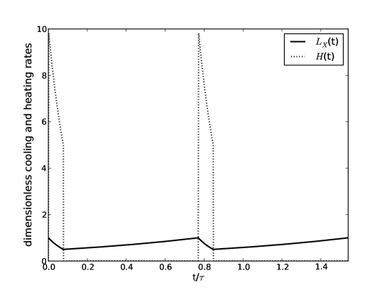
Figure 1: Two heating/cooling cycles of the X-ray luminosity, $L_{\rm X}(t)$, and AGN heating rate, $H(t)$, for a first-order, linear feedback system, subject to the minimum energy constraint. The values on the $y$-axis are given by $L_{\rm X}(t)/L_{\rm X}(t_{0})$ and $H(t)/L_{\rm X}(t_{0})$, while the x-axis is in units of the characteristic timescale of the system, $\tau$. In this example, the feedback strength is $k_{1}=10$, so that duty cycle is $\delta\approx 0.1$.

Under the assumption of periodic heating, the energy injected by the AGN each cycle is the same as the energy radiated by the gas. For optimal heating, this quantity is $E_{\rm heat}=E_{\rm cool}=L_{\rm X}(t_{0})\tau k_{1}/[2(k_{1}-1)]$. Thus, the total energy produced each cycle, is $E_{\rm out}=E_{\rm heat}+E_{\rm cool}=L_{\rm X}(t_{0})\tau k_{1}/(k_{1}-1)$. In addition, given that the time-averaged AGN power output is rate is $\langle H\rangle=E_{\rm heat}/(t_{1}-t_{0})$, the time-averaged black hole growth rate must be $\langle\dot{M}_{\rm BH}\rangle=\langle H\rangle/(\eta c^{2})=L_{\rm X}(t_{0})/(\eta c^{2}\ln 4)$, where $\eta$ is the standard accretion efficiency and $c$ is the speed of light. During the accretion phase, the average accretion rate of the black hole growth rate is a factor $k_{1}=1/\delta$ greater, and can be approximated by $\dot{M}_{\rm BH}=L_{\rm X}(t_{0})/(\delta\eta c^{2}\ln 4)$. Consequently, systems with characteristically small duty cycles will experience brief phases of rapid black hole growth. In contrast, black hole growth in systems with duty cycles closer to unity will be much more uniform.

4 Discussion

Observationally, the radio AGN duty cycle is found to increase steeply with the stellar mass of the host galaxy (e.g. Best et al., 2005), and is higher still for Brightest Cluster Galaxies (Best et al., 2007). In the context of the model presented here, this suggests that the feedback strength decreases with increasing stellar mass.

If the argument above holds, the ratio of the instantaneous heating and cooling rates ($H/L_{\rm X}=k_{1}$) will also decrease with increasing stellar mass of the host galaxy. Consequently, lower mass systems must experience proportionally more powerful heating events. As a result, the momentum and energy supplied by the AGN would be much more capable of expelling X-ray emitting material from the gravitational potential of an elliptical galaxy than a galaxy cluster. This scenario would appear to be consistent with recent theoretical interpretations of the steepening of the $L_{\rm X}-T$ relation below 1-2 keV (e.g. Puchwein et al., 2008; Bower et al., 2008; Pope, 2009).

A plausible relationship between $k_{1}$ and the average temperature of the ambient gas, is as follows. When activated, the AGN heating rate is assumed to be proportional to the X-ray luminosity, such that $H(t)=\eta\dot{M}_{\rm BH}c^{2}=k_{1}L_{\rm X}(t)$, where $\dot{M}_{\rm BH}$ is the black hole fuelling rate, and the other quantities are as previously defined. The classical mass flow rate for an X-ray emitting atmosphere with luminosity $L_{\rm X}(t)$, and average temperature $T$, is defined as $L_{\rm X}=(5/2)k_{\rm B}T\dot{M}_{\rm clas}/\mu m_{\rm p}$, where $k_{\rm B}$ is the Boltzmann constant and $\mu m_{\rm p}$ is the mean mass per particle. Thus, if a fraction, $\phi$, of the classical mass flow rate reaches the supermassive black hole, we can write $\dot{M}_{\rm BH}=\phi\dot{M}_{\rm clas}$, and it can be shown that $k_{1}=2\phi\eta\mu m_{\rm p}c^{2}/(5k_{\rm B}T)$. Therefore, stronger feedback (and smaller duty cycles) should be observed in cooler, less massive systems, as is consistent with standard interpretations of radio AGN observations (Best et al., 2005, 2007; Shabala et al., 2008).

To calculate a numerical value for $k_{1}$, we assume a canonical accretion efficiency of $\eta=0.1$, which yields $k_{1}=1/\delta\approx 260(\phi/0.01)(T/10^{7}\,{\rm K})^{-1}$. For low mass elliptical galaxies, Best et al. (2005) found $\delta\sim 10^{-4}-10^{-3}$ which, in the context of the present model suggests $k_{1}\sim 10^{3}-10^{4}$. Thus, for a characteristic X-ray temperature of $T\sim 10^{6}\,{\rm K}$, a value of $k_{1}\sim 10^{3}-10^{4}$ can only be obtained if $\phi\sim 10^{-2}$. In contrast, the duty cycle of radio AGN activity in Brightest Cluster Galaxies is $\delta\sim 0.1-1$ (e.g. Best et al., 2007), suggesting that $k_{1}\sim 1-10$. Given that the typical X-ray temperature in such systems is $T\sim 10^{8}\,{\rm K}$, the fraction of the classical cooling flow rate accreted by the black hole must be $\phi\sim 10^{-4}-10^{-3}$.

If the reasoning outlined above approximates reality, we might infer that the accreted fraction, $\phi$, tends to decrease in hotter (more spatially extended) systems. The simplest qualitative explanation for such a phenomenon is that the black hole predominantly accretes material from the central region of a galaxy or cluster. Therefore, the fraction of material accreted from the entire cooling flow will be governed by the size of this central region relative to the size of the region within which the classical cooling flow rate applies.

5 Summary

The aim of this article has been to demonstrate how standard techniques optimal control theory can be used to investigate some of the fundamental characteristics of feedback which may be applicable to AGN heating in massive galaxies and galaxy clusters. Although it has not yet been possible to construct a completely satisfactory model for AGN heating, the application of optimal control theory has elucidated some potentially important features of constrained feedback systems. The main findings are described below.

1. Optimal control theory provides a way to impose additional constraints on the system, with the minimum number of assumptions. In general terms, constraints are extremely useful for conceptualising the interaction between the AGN and its environment and interpreting observational signatures. More specifically, we have shown that AGN heating (regulated by feedback) which acts to minimise the total energy output of the system, occurs in the form of discrete, periodic events. This constraint ensures that AGN heating balances gas cooling with the minimum black hole growth and produces behaviour which is broadly compatible with a range of observations. However, this is only one interpretation and explanation of the observations. In principle, there may be other effects or constraints which achieve similar outcomes.

2. The duty cycle for periodic AGN activity in a first-order, linear feedback system is $\delta\approx 1/k_{1}$, where $k_{1}$ is the feedback strength. If this interpretation is applied to observations which show radio AGN duty cycles increasing with the stellar mass of the host galaxy (Best et al., 2005, 2007; Shabala et al., 2008), we would infer that the feedback strength decreases as the system stellar mass increases. In turn, this would mean that AGN outbursts in lower mass systems are proportionally stronger than those in more massive environments so that AGN heating events may be sufficiently powerful to expel hot gas from the gravitational potential of a galaxy, but not a galaxy cluster. A description of this sort is in qualitative agreement with recent theoretical explanations for the steepening of the $L_{\rm X}-T$ relation for temperatures below 1-2 keV (e.g. Puchwein et al., 2008; Bower et al., 2008; Pope, 2009).

6 Acknowledgements

The author would like to thank CITA for funding through a National Fellowship.

References

- Alexander (1996) Alexander R., 1996, Optima for Animals. Princeton University Press
- Bîrzan et al. (2004) Bîrzan L., Rafferty D. A., McNamara B. R., Wise M. W., Nulsen P. E. J., 2004, ApJ, 607, 800
- Benson et al. (2003) Benson A. J., Bower R. G., Frenk C. S., Lacey C. G., Baugh C. M., Cole S., 2003, ApJ, 599, 38
- Best (2007) Best P. N., 2007, New Astronomy Review, 51, 168
- Best et al. (2005) Best P. N., Kauffmann G., Heckman T. M., Brinchmann J., Charlot S., Ivezić Ž., White S. D. M., 2005, MNRAS, 362, 25
- Best et al. (2007) Best P. N., von der Linden A., Kauffmann G., Heckman T. M., Kaiser C. R., 2007, MNRAS, 379, 894
- Binney & Tabor (1995) Binney J., Tabor G., 1995, MNRAS, 276, 663
- Bower et al. (2006) Bower R. G., Benson A. J., Malbon R., Helly J. C., Frenk C. S., Baugh C. M., Cole S., Lacey C. G., 2006, MNRAS, 370, 645
- Bower et al. (2008) Bower R. G., McCarthy I. G., Benson A. J., 2008, MNRAS, 390, 1399
- Bregman & David (1988) Bregman J. N., David L. P., 1988, ApJ, 326, 639
- Burghes & Downs (1975) Burghes D. N., Downs A. M., 1975, Modern Introduction to Classical Mechanics, Control Mathematics and Its Applications. Ellis Horwood Ltd
- Burns (1990) Burns J. O., 1990, ApJ, 99, 14
- Cavagnolo et al. (2008) Cavagnolo K. W., Donahue M., Voit G. M., Sun M., 2008, ApJ, 683, L107
- Cho et al. (2003) Cho J., Lazarian A., Honein A., Knaepen B., Kassinos S., Moin P., 2003, ApJ, 589, L77
- Ciotti & Ostriker (2001) Ciotti L., Ostriker J. P., 2001, ApJ, 551, 131
- Croton et al. (2006) Croton D. J., Springel V., White S. D. M., De Lucia G., Frenk C. S., Gao L., Jenkins A., Kauffmann G., Navarro J. F., Yoshida N., 2006, MNRAS, 365, 11
- DiStefano et al. (1994) DiStefano J. J., Stubberud A. R., Williams I. J., 1994, Feedback and control systems. McGraw-Hill
- Dunn & Fabian (2008) Dunn R. J. H., Fabian A. C., 2008, MNRAS, 385, 757
- Dunn et al. (2005) Dunn R. J. H., Fabian A. C., Taylor G. B., 2005, MNRAS, 364, 1343
- Fabjan et al. (2010) Fabjan D., Borgani S., Tornatore L., Saro A., Murante G., Dolag K., 2010, MNRAS, 401, 1670
- Fairman (1998) Fairman F. W., 1998, Linear Control Theory: The State Space Approach. John Wiley and Sons
- Fujita & Reiprich (2004) Fujita Y., Reiprich T. H., 2004, ApJ, 612, 797
- Gaetz (1989) Gaetz T. J., 1989, ApJ, 345, 666
- Guo et al. (2008) Guo F., Oh S. P., Ruszkowski M., 2008, ApJ, 688, 859
- Haggag & Safko (2003) Haggag S., Safko J. L., 2003, Ap. & Sp. Sci., 283, 369
- Heinz et al. (2006) Heinz S., Brüggen M., Young A., Levesque E., 2006, MNRAS, 373, L65
- Kaastra et al. (2004) Kaastra J. S., Tamura T., Peterson J. R., Bleeker J. A. M., Ferrigno C., Kahn S. M., Paerels F. B. S., Piffaretti R., Branduardi-Raymont G., Böhringer H., 2004, A&A, 413, 415
- Kaiser (2007) Kaiser C. R., 2007, Astronomy and Geophysics, 48, 040000
- Kirk (2004) Kirk D. E., 2004, Optimal Control Theory: An Introduction. Dover publications
- Mittal et al. (2009) Mittal R., Hudson D. S., Reiprich T. H., Clarke T., 2009, A&A, 501, 835
- Nulsen et al. (2007) Nulsen P. E. J., Jones C., Forman W. R., David L. P., McNamara B. R., Rafferty D. A., Bîrzan L., Wise M. W., 2007, in Böhringer H., Pratt G. W., Finoguenov A., Schuecker P., eds, Heating versus Cooling in Galaxies and Clusters of Galaxies AGN Heating Through Cavities and Shocks. pp 210–+
- Parrish et al. (2009) Parrish I. J., Quataert E., Sharma P., 2009, ApJ, 703, 96
- Peterson & Fabian (2006) Peterson J. R., Fabian A. C., 2006, Physical Reports, 427, 1
- Peterson et al. (2003) Peterson J. R., Kahn S. M., Paerels F. B. S., Kaastra J. S., Tamura T., Bleeker J. A. M., Ferrigno C., Jernigan J. G., 2003, ApJ, 590, 207
- Peterson et al. (2001) Peterson J. R., Paerels F. B. S., Kaastra J. S., Arnaud M., Reiprich T. H., Fabian A. C., Mushotzky R. F., Jernigan J. G., Sakelliou I., 2001, A&A, 365, L104
- Pope (2009) Pope E. C. D., 2009, MNRAS, pp 494–+
- Pope et al. (2005) Pope E. C. D., Pavlovski G., Kaiser C. R., Fangohr H., 2005, MNRAS, 364, 13
- Pope et al. (2006) Pope E. C. D., Pavlovski G., Kaiser C. R., Fangohr H., 2006, MNRAS, 367, 1121
- Puchwein et al. (2008) Puchwein E., Sijacki D., Springel V., 2008, ApJ, 687, L53
- Rafferty et al. (2008) Rafferty D. A., McNamara B. R., Nulsen P. E. J., 2008, ApJ, 687, 899
- Sakelliou et al. (2002) Sakelliou I., Peterson J. R., Tamura T., Paerels F. B. S., Kaastra J. S., Belsole E., Böhringer H., Branduardi-Raymont G., Ferrigno C., den Herder J. W., Kennea J., Mushotzky R. F., Vestrand W. T., Worrall D. M., 2002, A&A, 391, 903
- Shabala et al. (2008) Shabala S. S., Ash S., Alexander P., Riley J. M., 2008, MNRAS, 388, 625
- Short & Thomas (2009) Short C. J., Thomas P. A., 2009, ApJ, 704, 915
- Tamura et al. (2001) Tamura T., Kaastra J. S., Peterson J. R., Paerels F. B. S., Mittaz J. P. D., Trudolyubov S. P., Stewart G., Fabian A. C., Mushotzky R. F., Lumb D. H., Ikebe Y., 2001, A&A, 365, L87
- Tucker & David (1997) Tucker W., David L. P., 1997, ApJ, 484, 602
- Voigt & Fabian (2004) Voigt L. M., Fabian A. C., 2004, MNRAS, 347, 1130
- Xu et al. (2002) Xu H., Kahn S. M., Peterson J. R., Behar E., Paerels F. B. S., Mushotzky R. F., Jernigan J. G., Brinkman A. C., Makishima K., 2002, ApJ, 579, 600
- Zakamska & Narayan (2003) Zakamska N. L., Narayan R., 2003, ApJ, 582, 162