A new numerical strategy with space-time adaptivity and error control for multi-scale streamer discharge simulations

Abstract

This paper presents a new resolution strategy for multi-scale streamer discharge simulations based on a second order time adaptive integration and space adaptive multiresolution. A classical fluid model is used to describe plasma discharges, considering drift-diffusion equations and the computation of electric field. The proposed numerical method provides a time-space accuracy control of the solution, and thus, an effective accurate resolution independent of the fastest physical time scale. An important improvement of the computational efficiency is achieved whenever the required time steps go beyond standard stability constraints associated with mesh size or source time scales for the resolution of the drift-diffusion equations, whereas the stability constraint related to the dielectric relaxation time scale is respected but with a second order precision. Numerical illustrations show that the strategy can be efficiently applied to simulate the propagation of highly nonlinear ionizing waves as streamer discharges, as well as highly multi-scale nanosecond repetitively pulsed discharges, describing consistently a broad spectrum of space and time scales as well as different physical scenarios for consecutive discharge/post-discharge phases, out of reach of standard non-adaptive methods.

1 Introduction

In recent years, plasma discharges at atmospheric pressure have been studied for an increasing list of applications such as chemical and biological decontamination, aerodynamic flow control and combustion [1, 2]. In all these physical configurations, the discharges take usually the form of thin plasma filaments driven by highly nonlinear ionizing waves, also called streamers. These ionizing waves occur as a consequence of the high electric field induced by the fast variations of the net charge density ahead of an electron avalanche with large amplification. The streamer discharge dynamics are mainly governed by the Courant, the effective ionization and the dielectric relaxation times scales [3], which are usually of the order of $10^{-14}-10^{-12}$s, whereas the typical time scale of the discharge propagation in centimeter gaps, is about a few tens of nanoseconds. On the other hand, a large variation of space scales needs also to be taken into account, since the Debye length at atmospheric pressure can be as small as a few micrometers, while the inter-electrode gaps, where discharges propagate, are usually of the order of a few centimeters. As a result, the detailed physics of the discharges reveals an important time-space multi-scale character [4, 5].

More complex applications include plasma assisted combustion or flow control, for which the enhancement of the gas flow chemistry or momentum transfer during typical time scales of the flow of $10^{-4}-10^{-3}$s, is due to consecutive discharges generated by high frequency (in the kHz range) sinusoidal or pulsed applied voltages [6, 7]. Therefore, during the post-discharge phases of the order of tens of microseconds, not only the time scales are very different from those of the discharge phases of a few tens of nanoseconds, but a completely different physics is taking place. Then, to the rapid multi-scale configuration during discharges, we have to add other rather slower multi-scale phenomena in the post-discharge, such as recombination of charged species, heavy-species chemistry, diffusion, gas heating and convection. Therefore, it is very challenging to accurately simulate the physics of plasma/flow interactions due to the synergy effects between the consecutive discharge/post-discharge phases.

In most numerical models of streamer discharges, the motion of electrons and ions is governed by drift-diffusion equations coupled with Poisson’s equation. Early simulation studies were limited to simplified situations where the streamer is considered as a cylinder of constant radius [8, 9, 10, 11], in which the charged particle densities are assumed to be constant along the radial extension of the streamer: the 1.5D model approach. In this model, the spatio-temporal evolution of the charged particle densities is solved only along one spatial dimension in the direction of propagation, whereas the electric field is calculated in two dimensions using the so-called disc method, based on a direct integration of analytical results. A 2D model for the electric field is indeed essential to properly calculate the electric field enhancement by the space charge in the streamer head. After the first 2D streamer simulations using the Poisson’s equation resolution were performed [12], many studies have been carried out in 2D [3, 13, 14, 15, 16, 17, 18] and 3D [19, 20, 21, 22].

Being aware of the complexity of fully coupled resolutions of these modeling equations, a decoupling strategy is usually adopted, which considers an independent and successive numerical resolution of Poisson’s equation with a fixed charge distribution, and of the drift-diffusion equations with a fixed electric field during each decoupling time step. These computations might be performed explicitly in time with standard first or even second order schemes [23, 24]. In these cases, the time steps are usually limited for the sake of stability by the various characteristic times scales (Courant, ionization, dielectric relaxation), whereas the accuracy of simulations is assumed to be given by the resolution of the fastest physical time scale. In order to somehow overcome the dielectric relaxation limitation, some semi-implicit approaches were developed [25, 26, 27], based on a predictive approximation of the space charge ahead in time during the electric field computation, even though the other time scale constraints remain. This gain of stability allows important improvements in terms of computational efficiency but the accuracy of simulations becomes rather difficult to quantify.

Another performing technique to improve the efficiency of simulations considers an asynchronous explicit time integration of the drift-diffusion equations with self-adaptive local time-stepping, for which the local time steps are based either on local dynamic increments of the solution [28, 29] or on local Courant conditions [30]. These techniques are the subject of several studies [31, 32, 33] and are mainly conceived to avoid expensive computations whenever the whole system is unnecessarily advanced in time with a global time step prescribed by the fastest scale. Even though these methods yield efficient strategies, specially in terms of CPU time savings, with stable and flux-conserving time integrations, it is rather difficult to conduct an accuracy control on the resolution of the time dependent equations or on their coupling with the electric field resolution for plasma models.

In this work, a numerical study is conducted in order to build a second order explicit in time decoupling scheme for the resolution of the electric field and the electron and ion densities. A lower order and embedded method is taken into account to dynamically compute the decoupling time steps that guarantee an accurate description with error control of the global physical coupling. At this stage, the only limiting time scale is the dielectric relaxation characteristic time for stability reasons. In a second level, the drift-diffusion equations are solved using a Strang second order operator splitting scheme in order to guarantee the global order of the strategy [34, 35]. This time integration scheme considers high order dedicated methods during each splitting time step, which is dynamically adapted by an error control procedure [36]. In this way, even though there is a global advance in time given by the splitting time step, the latter is determined by the desired accuracy of the global physics, which is not necessarily related to the stability constraints associated with the mesh size or the fastest source time scales as demonstrated in [37]. As a consequence, this technique provides an error control procedure and stands as an alternative way to local stepping schemes to overcome time step limitations related to the reaction, diffusion and convection phenomena.

Both the electric field and density resolutions are performed on an adapted mesh obtained by a spatial multiresolution method, based on Harten’s pioneering work [38] and further developed in [39], taking into account the spatial multi-scale features of these phenomena with steep spatial gradients. In particular, some grid adaptation techniques for 2D structured meshes were already used [23, 4, 20] and extensions to 3D have been also proposed [20, 19] for streamer simulations. However, one of the main advantages of the multiresolution approach is that it is based on a wavelet representation technique and an error of the spatial approximation can be then mathematically estimated. Consequently, an effective error control is achieved for both the time and space resolution of the multi-scale phenomena under study.

The performance of the method is first evaluated for a propagating streamer problem with the multi-scale features previously discussed, for which the various simulation parameters are studied. Once the physical configuration is settled, a 1.5D streamer model is adopted in order to obtain an electric field resolution strategy based on direct computations and derived from analytical expressions, suitable for adapted finite volume discretizations [40]. In a second step, a more complex physical configuration is considered for the simulation of repetitively pulsed discharges, for which a time-space adaptive method is required to efficiently overcome some highly multi-scale features in order to fully describe the various physical phenomena. In this work, only a 1.5D model is considered but extensions to higher dimensions is straightforward for instance with a Poisson’s equation solver for adapted grids as it has been implemented in [23, 4, 20]. However, in this paper we focus on the development and validation of new numerical methods for the resolution of the drift-diffusion equations and its coupling with the electric field computation, which are independent of the dimension of the problem. Numerical illustrations of multidimensional problems with the same time-space adaptive strategy with error control will be the subject of future work.

The paper is organized as follows: in Section 2, we present the physical configuration and the modeling equations. The numerical strategy is presented in Section 3, in which the second order adaptive time integration technique is detailed along with the resolution of drift-diffusion equations and the electric field, as well as the spatial multiresolution adaptive procedure. Numerical illustrations are summarized in Section 4 for two configurations given by single propagating and multi-pulsed discharges. We end with some concluding remarks and prospects on future developments and applications.

2 Model formulation

In this work, we consider positive streamer discharges in air at atmospheric pressure in a point-to-plane geometry, as shown in Figure 1. The tip of the anode is placed $1\,$cm from the planar cathode and the radius of curvature of the anode is $324\,\mu$m. The most common and effective model to study streamer dynamics is based on the following drift-diffusion equations for electrons and ions, coupled with Poisson’s equation [41, 42]:

$$\left.\begin{array}[]{rcl}\partial_{t}n_{\rm e}-\partial_{\bf x}\cdot n_{\rm e}\,{\bf v}_{\!\rm e}-\partial_{\bf x}\cdot(D_{\rm e}\ \partial_{\bf x}n_{\rm e})&=&n_{\rm e}\alpha|{\bf v}_{\rm e}|-n_{\rm e}\eta|{\bf v}_{\rm e}|+n_{\rm e}n_{\rm p}\beta_{\rm ep}+n_{\rm n}\gamma,\\ \partial_{t}n_{\rm p}+\partial_{\bf x}\cdot n_{\rm p}{\bf v}_{\!\rm p}-\partial_{\bf x}\cdot(D_{\rm p}\,\partial_{\bf x}n_{\rm p})&=&n_{\rm e}\alpha|{\bf v}_{\rm e}|-n_{\rm e}n_{\rm p}\beta_{\rm ep}+n_{\rm n}n_{\rm p}\beta_{\rm np},\\ \partial_{t}n_{\rm n}-\partial_{\bf x}\cdot n_{\rm n}{\bf v}_{\!\rm n}-\partial_{\bf x}\cdot(D_{\rm n}\,\partial_{\bf x}n_{\rm n})&=&n_{\rm e}\eta|{\bf v}_{\rm e}|-n_{\rm n}n_{\rm p}\beta_{\rm np}-n_{\rm n}\gamma,\end{array}\right\}$$ (1)

$$\varepsilon_{0}\,\partial_{\bf x}^{2}V=-q_{\rm e}(n_{\rm p}-n_{\rm n}-n_{\rm e}),$$ (2)

where ${\bf x}\in\mathbb{R}^{d}$, $n_{i}$ is the density of species $i$ (e: electrons, p: positive ions, n: negative ions), $V$ is the electric potential, ${\bf v}_{i}=\mu_{i}{\bf E}$ (${\bf E}$ being the electric field) is the drift velocity. $D_{i}$ and $\mu_{i}$, are the diffusion coefficient and the absolute value of mobility of the charged species $i$, $q_{\rm e}$ is the absolute value of an electron charge, and $\varepsilon_{0}$ is the permittivity of free space. $\alpha$ is the impact ionization coefficient, $\eta$ stands for the electron attachment on neutral molecules, $\beta_{\rm ep}$ and $\beta_{\rm np}$ account respectively for the electron-positive ion and the negative-positive ion recombination, and $\gamma$ is the detachment coefficient.

Figure 1: Computational domain for the studied point-to-plane geometry.

The electric field ${\bf E}$ and the potential $V$ are related by

$${\bf E}=-\partial_{\bf x}V,$$ (3)

and thus, the Poisson’s equation (2) becomes:

$$\varepsilon_{0}\,\partial_{\bf x}\cdot{\bf E}=q_{\rm e}(n_{\rm p}-n_{\rm n}-n_{\rm e}).$$ (4)

All the coefficients of the model are assumed to be functions of the local reduced electric field $E/N_{\rm gas}$, where $E$ is the electric field magnitude and $N_{\rm gas}$ is the air neutral density. For test studies presented in this paper, the transport parameters for air are taken from [43]; detachment and attachment coefficients, respectively from [44] and [45]; and other reaction rates, also from [43]. Diffusion coefficients for ions are derived from mobilities using classical Einstein relations.

In simulations of positive streamer discharges in air at atmospheric pressure without any preionization, the photoionization term is crucial to produce seed charges in front of the streamer head and then to ensure the streamer propagation [24]. However, in repetitive discharges, [46] and recently [47] have shown that even at low frequency, a significant amount of seed charges from previous discharges may be present in the inter-electrode gap. In this work, we have neglected the photoionization source term and considered discharge conditions with a preionization background to ensure a stable propagation of the discharge without impacting the main discharge characteristics [15, 46, 18, 48].

3 Construction of the numerical strategy

In this section, we introduce a new numerical technique for multi-scale streamer discharge simulations, based on a second order decoupled resolution of the electric field and the drift-diffusion equations for electrons and ions, with self-adaptive decoupling time steps with error control. The drift-diffusion equations are then solved using a dedicated Strang time operator splitting scheme for multi-scale phenomena. On the other hand, the electric field is computed based on a parallel computing method, specially conceived for the configuration under study in 1.5D geometry. Both resolutions are conducted on a dynamic adaptive mesh using spatial multiresolution transformation with error control of the spatial adapted representation.

3.1 Second order adaptive time integration strategy

Let us write the semi-discretized equations (1) and (4) in the following way just for analysis purposes:

$$\left.\begin{array}[]{rcl}{\rm d}_{t}\psi&=&\Psi(\psi,\phi),\\ 0&=&\Phi(\psi,\phi),\end{array}\right\}$$ (5)

for $t>t_{0}$, where $\psi:\mathbb{R}\to\mathbb{R}^{N\times m}$ and $\phi:\mathbb{R}\to\mathbb{R}^{N\times d}$ stand respectively for the spatial discretization of $(n_{\rm e},n_{\rm p},n_{\rm n})$, i.e. $m=3$, and of ${\bf E}$ over $N$ points. Supposing that all functions are sufficiently differentiable in all their variables and using the Taylor expansion of the true solution, one can write after some time $\Delta t$ from initial time $t_{0}$,

$$\psi(t_{0}+\Delta t)=\psi_{0}+\Delta t\Psi(\psi_{0},\phi_{0})+\displaystyle{\frac{\Delta t^{2}}{2}}\left[\partial_{\psi}\Psi\,\Psi+\partial_{\phi}\Psi\,{\rm d}_{t}\phi\right]_{t=t_{0}}+\mathcal{O}(\Delta t^{3}),$$ (6)

with $\psi_{0}=\psi(t_{0})$, $\phi_{0}=\phi(t_{0})$.

A second order in time resolution of system (5) must then verify (6) locally for each $\Delta t$. However, as it was stated before, solving simultaneously (1) and (2) (or (4)), or equivalently (5), involves important numerical difficulties, considering for instance the different nature of equations (1) and (2) (or (4)). Therefore, a decoupled approach is often used in which one aims at solving the drift-diffusion equations and the electric field independently. This amounts to solve

$${\rm d}_{t}\tilde{\psi}=\Psi(\tilde{\psi},\phi^{\star}),\quad t\in\,]t_{0},t_{0}+\Delta t],$$ (7)

with fixed $\phi^{\star}=\phi(t^{\star})$, $t^{\star}\in[t_{0},t_{0}+\Delta t]$ and $\tilde{\psi}(t_{0})=\psi_{0}$.

The most common technique considers $t^{\star}=t_{0}$, that is, to previously compute the electric field at $t_{0}$ from $\Phi(\psi_{0},\phi_{0})=0$, and then solve (7) with $\phi^{\star}=\phi_{0}$. This can be interpreted as a standard first order operator splitting method that yields an approximation of order 1, $\tilde{\psi}_{1}(t)$, of the exact solution, $\psi(t)$, based on classical numerical analysis results obtained by confronting (6) with

$$\tilde{\psi}_{1}(t_{0}+\Delta t)=\psi_{0}+\Delta t\Psi(\psi_{0},\phi_{0})+\displaystyle{\frac{\Delta t^{2}}{2}}\left[\partial_{\psi}\Psi\,\Psi\right]_{t=t_{0}}+\mathcal{O}(\Delta t^{3}).$$ (8)

The same result follows for $\tilde{\phi}_{1}(t_{0}+\Delta t)$ computed out of $\Phi(\tilde{\psi}_{1}(t_{0}+\Delta t),\tilde{\phi}_{1}(t_{0}+\Delta t))=0$ or equivalently, out of its explicit representation $\tilde{\phi}_{1}(t_{0}+\Delta t)=\Upsilon(\tilde{\psi}_{1}(t_{0}+\Delta t))$, assuming a Lipschitz condition:

$$\left\|\Upsilon(\psi)-\Upsilon(\psi^{\star})\right\|\leq L\left\|\psi-\psi^{\star}\right\|.$$ (9)

Considering now any $t^{\star}\in[t_{0},t_{0}+\Delta t]$ into (7), the only second order solution, $(\tilde{\psi}_{2}(t),\tilde{\phi}_{2}(t))$, will be given by resolution of (7) with $\phi^{\star}=\phi_{\frac{1}{2}}$ for $t^{\star}=t_{0}+\Delta t/2$, for which

$$\tilde{\psi}_{2}(t_{0}+\Delta t)=\psi_{0}+\Delta t\Psi(\psi_{0},\phi_{\frac{1}{2}})+\displaystyle{\frac{\Delta t^{2}}{2}}\left[\partial_{\psi}\Psi\,\Psi\right]_{\psi\to\psi_{0},\phi_{\frac{1}{2}}}+\mathcal{O}(\Delta t^{3}),$$ (10)

where

$$\Psi(\psi_{0},\phi_{\frac{1}{2}}) = \Psi\left(\psi_{0},\phi\left(t_{0}+\frac{\Delta t}{2}\right)\right)$$ (11)

$$= \Psi\left(\psi_{0},\phi_{0}+\displaystyle{\frac{\Delta t}{2}}\left.{\rm d}_{t}\phi\right|_{t=t_{0}}+\mathcal{O}(\Delta t^{2})\right)$$

$$= \Psi(\psi_{0},\phi_{0})+\displaystyle{\frac{\Delta t}{2}}\left[\partial_{\phi}\Psi\,{\rm d}_{t}\phi\right]_{t=t_{0}}+\mathcal{O}(\Delta t^{2}),$$

and hence,

$$\tilde{\psi}_{2}(t_{0}+\Delta t)=\psi_{0}+\Delta t\Psi(\psi_{0},\phi_{0})+\displaystyle{\frac{\Delta t^{2}}{2}}\left[\partial_{\psi}\Psi\,\Psi+\partial_{\phi}\Psi\,{\rm d}_{t}\phi\right]_{t=t_{0}}+\mathcal{O}(\Delta t^{3});$$ (12)

and

$$\tilde{\phi}_{2}(t_{0}+\Delta t)=\Upsilon(\tilde{\psi}_{2}(t_{0}+\Delta t)).$$ (13)

Nevertheless, this second order approximation, $\tilde{\psi}_{2}(t)$, is based on the previous knowledge of $\phi_{\frac{1}{2}}=\phi(t_{0}+\Delta t/2)$, and thus, of $\psi(t_{0}+\Delta t/2)$. In order to overcome this difficulty, one can solve (7) with $\phi^{\star}=\tilde{\phi}_{1}(t_{0}+\Delta t/2)=\Upsilon(\tilde{\psi}_{1}(t_{0}+\Delta t/2))$, that is, computing first $\tilde{\psi}_{1}(t_{0}+\Delta t/2)$ with the first order method. In particular, this does not change the previous order estimates as it follows from

$$\psi(t_{0}+\Delta t)-\tilde{\psi}_{2}(t_{0}+\Delta t) = \displaystyle{\frac{\Delta t^{2}}{2}}\left[\partial_{\phi}\Psi\,{\rm d}_{t}(\phi-\tilde{\phi}_{1})\right]_{t=t_{0}}+\mathcal{O}(\Delta t^{3})$$ (14)

$$= \displaystyle{\frac{\Delta t^{2}}{2}}\left[\partial_{\phi}\Psi\,\partial_{\psi}\Upsilon\,{\rm d}_{t}(\psi-\tilde{\psi}_{1})\right]_{t=t_{0}}+\mathcal{O}(\Delta t^{3})$$

$$= \mathcal{O}(\Delta t^{3}).$$

Taking into account both methods,

$$\left(\begin{array}[]{c}\tilde{\psi}_{1}(t_{0}+\Delta t)\\ \tilde{\phi}_{1}(t_{0}+\Delta t)\end{array}\right)=\mathcal{T}_{1}^{\Delta t}\left(\begin{array}[]{c}\psi_{0}\\ \phi_{0}\end{array}\right),\quad\left(\begin{array}[]{c}\tilde{\psi}_{2}(t_{0}+\Delta t)\\ \tilde{\phi}_{2}(t_{0}+\Delta t)\end{array}\right)=\mathcal{T}_{2}^{\Delta t}\left(\begin{array}[]{c}\psi_{0}\\ \phi_{0}\end{array}\right),$$ (15)

we perform computations with a second order scheme $\mathcal{T}_{2}^{\Delta t}$, which uses an embedded and lower order scheme $\mathcal{T}_{1}^{\Delta t/2}$, as it was previously detailed. An adaptive time step strategy is then implemented in order to control the accuracy of computations by tuning the duration of the decoupled resolution. It is based on a local error estimate, dynamically computed at the end of each decoupling time step $\Delta t$, given by

$$\big{\|}\mathcal{T}_{2}^{\Delta t}(\psi_{0},\phi_{0})^{t}-\mathcal{T}_{1}^{\Delta t}(\psi_{0},\phi_{0})^{t}\big{\|}\approx\mathcal{O}({\Delta t}^{2}).$$ (16)

Therefore, for a given accuracy tolerance $\eta_{\mathcal{T}}$,

$$\big{\|}\mathcal{T}_{2}^{\Delta t}(\psi_{0},\phi_{0})^{t}-\mathcal{T}_{1}^{\Delta t}(\psi_{0},\phi_{0})^{t}\big{\|}<\eta_{\mathcal{T}}$$ (17)

must be verified in order to accept the current computation with $\Delta t$, while the new time step is calculated by

$$\Delta t^{\rm new}=\Delta t\sqrt{\frac{\eta_{\mathcal{T}}}{\big{\|}\mathcal{T}_{2}^{\Delta t}(\psi_{0},\phi_{0})^{t}-\mathcal{T}_{1}^{\Delta t}(\psi_{0},\phi_{0})^{t}\big{\|}}}.$$ (18)

Several dedicated solvers can be then implemented for each subproblem (1) and (2) while the theoretical error estimates of the decoupling schemes analyzed in this section remain valid. In this way, the independent choice of appropriate numerical schemes allows to strongly reduce the computational complexity of the global numerical strategy, and an error control procedure such as the one proposed in this work allows to effectively calibrate this decoupling within a prescribed accuracy tolerance.

3.2 Resolution of the drift-diffusion equations

We consider now the numerical resolution of the drift-diffusion equations (1), that can be written in the general form of a convection-reaction-diffusion system of equations:

$$\left.\begin{array}[]{rcll}\displaystyle{\partial_{t}{\bf u}-\partial_{{\bf x}}\left({\bf F}\left({\bf u}\right)+{\bf D}({\bf u})\partial_{{\bf x}}{\bf u}\right)}&=&{\displaystyle{\bf f}\left({\bf u}\right),}&t>t_{0},\\ \displaystyle{{\bf u}(t_{0},{\bf x})}&=&{\displaystyle{\bf u}_{0}({\bf x}),}&t=t_{0},\end{array}\right\}$$ (19)

where ${\bf F}$, ${\bf f}:\mathbb{R}^{m}\to\mathbb{R}^{m}$ and ${\bf u}:\mathbb{R}\times\mathbb{R}^{d}\to\mathbb{R}^{m}$, with a tensor of order $d\times d\times m$ as diffusion matrix ${\bf D}({\bf u})$. In particular, ${\bf u}=(n_{\rm e},n_{\rm p},n_{\rm n})^{t}$ with $m=3$ in this study.

The system (19) corresponds to problem (7) for a fixed electric field, and it is solved during each decoupling time step $\Delta t$ into $\mathcal{T}_{2}$ (or $\mathcal{T}_{1}$) scheme, using a Strang time operator scheme with dedicated high order time integrators on a dynamic adaptive mesh, based on a strategy introduced in [34]. This resolution is briefly detailed in following sections.

3.2.1 Time operator splitting

An operator splitting procedure allows to consider dedicated solvers for the reaction part which is decoupled from other physical phenomena like convection, diffusion or both, for which there also exist dedicated numerical methods. These dedicated methods chosen for each subsystem are then responsible for dealing with the fastest scales associated with each one of them, in a separate manner, while the reconstruction of the global solution by the splitting scheme should guarantee an accurate description with error control of the global physical coupling, without being related to the stability constraints of the numerical resolution of each subsystem.

Considering problem (19) and in order to remain consistent with the second order $\mathcal{T}_{2}$ scheme, a second order Strang scheme is implemented [49]

$$\mathcal{S}^{\Delta t_{\rm s}}({\bf u}_{0})=\mathcal{R}^{\Delta t_{\rm s}/2}\mathcal{D}^{\Delta t_{\rm s}/2}\mathcal{C}^{\Delta t_{\rm s}}\mathcal{D}^{\Delta t_{\rm s}/2}\mathcal{R}^{\Delta t_{\rm s}/2}({\bf u}_{0}),$$ (20)

where operators $\mathcal{R}$, $\mathcal{D}$, $\mathcal{C}$ indicate respectively the independent resolution of the reaction, diffusion and convection problems with a splitting time step, $\Delta t_{\rm s}$, taken inside the overall decoupling time step, $\Delta t_{\rm s}\leq\Delta t$. Usually, for propagating reaction waves where for instance, the speed of propagation is much slower than some of the chemical scales, the fastest scales are not directly related to the global physics of the phenomenon, and thus, larger splitting time steps might be considered [34, 35]. Nevertheless, order reductions may then appear due to short-life transients associated with fast variables and in these cases, it has been proven in [50] that better performances are expected while ending the splitting scheme by operator $\mathcal{R}$ or in a more general case, the part involving the fastest time scales of the phenomenon.

The resolution of (19) should be precise enough to guarantee theoretical estimates given in Section 3.1. Therefore, an adaptive splitting time step strategy, based on a local error estimate at the end of each splitting time step $\Delta t_{\rm s}$, is also implemented in order to control the accuracy of computations [37]. In this context, a second, embedded and lower order Strang splitting method $\widetilde{\mathcal{S}}^{\Delta t_{\rm s}}$ was developed by [36], which allows to dynamically calculate a local error estimate that should verify

$$\big{\|}\mathcal{S}^{\Delta t_{\rm s}}({\bf u}_{0})-\widetilde{\mathcal{S}}^{\Delta t_{\rm s}}({\bf u}_{0})\big{\|}\approx\mathcal{O}({\Delta t_{\rm s}}^{2})<\eta_{\rm split},$$ (21)

in order to accept the current computation with $\Delta t_{\rm s}$, and thus, the new splitting time step is given by

$$\Delta t_{\rm s}^{\rm new}=\min\left(\Delta t_{\rm s}\sqrt{\frac{\eta_{\rm split}}{\big{\|}\mathcal{S}^{\Delta t_{\rm s}}({\bf u}_{0})-\widetilde{\mathcal{S}}^{\Delta t_{\rm s}}({\bf u}_{0})\big{\|}}},\ t_{0}+\Delta t-\hat{t}\right),$$ (22)

with $\eta_{\rm split}\leq\eta_{\mathcal{T}}$ and $\hat{t}=\sum_{i}\Delta t_{{\rm s}_{i}}$ while $\hat{t}\in\,]t_{0},t_{0}+\Delta t]$.

The choice of suitable time integration methods to numerically approximate $\mathcal{R}$, $\mathcal{D}$ and $\mathcal{C}$ during each $\Delta t_{\rm s}$ is mandatory not only to guarantee the theoretical framework of the numerical analysis but also to take advantage of the particular features of each independent subproblem. A new operator splitting for reaction-diffusion systems was recently introduced [34, 35], which considers a high fifth order, A-stable, L-stable method like Radau5 [51], based on implicit Runge-Kutta schemes for stiff ODEs, that solves with a local cell by cell approach the reaction term: a system of stiff ODEs without spatial coupling in a splitting context. For the diffusion problem, another high fourth order method like ROCK4 [52] is considered, which is based on explicit stabilized Runge-Kutta schemes that feature extended stability domains along the negative real axis. The ROCK4 solver is then very appropriate for diffusion problems because of the usual predominance of negative real eigenvalues. Both methods incorporate adaptive time integration tools, similar to (18) and (22), in order to control the accuracy of the integrations for given accuracy tolerances $\eta_{\rm Radau5}$ and $\eta_{\rm ROCK4}$, chosen such that $\eta_{\rm Radau5}<\eta_{\rm split}$ and $\eta_{\rm ROCK4}<\eta_{\rm split}$. In particular, in the case of multi-scale propagating waves, it can be proven that the local treatment plus the adaptive time stepping of the reaction solver allow to discriminate the cells of high reactive activity only present in the neighborhood of the localized wavefront, saving as a consequence a large quantity of integration time [35].

An explicit high order in time and in space one step monotonicity preserving scheme OSMP [53] is used as convective scheme. It combines monotonicity preserving constraints for non-monotone data to avoid extrema clipping, with TVD features to prevent spurious oscillations around discontinuities or sharp spatial gradients. Classical CFL stability restrictions are though imposed inside each splitting time step $\Delta t_{\rm s}$ for operator $\mathcal{C}^{\Delta t_{\rm s}}$. The overall combination of an explicit treatment of the spatial phenomena as convection and diffusion, with a local implicit integration of stiff reaction implies important savings in computing time and memory resources [34], as well as an important reduction of computational complexity with respect to a fully implicit coupled resolution of problem (19). On the other hand an explicit coupled treatment of (19) will have a very limited efficiency for stiff problems unless more sophisticated strategies as the asynchronous local time-stepping techniques [28, 29, 30] are considered even though these schemes do not provide a precise measurement of the accuracy of the integration.

Finally, the numerical errors of the splitting scheme are effectively handled by an error control procedure which furthermore allows to determine the coupling time scales of the global phenomenon that can be several orders of magnitude slower than the fastest time scales of each subproblem treated by each dedicated solver. In this way a decoupling of the time scale spectrum of the problem is achieved that leads to more efficient performances within a prescribed accuracy tolerance whenever this decomposition of scales is possible.

3.2.2 Mesh refinement technique

Regarding problem (19), we are concerned with the propagation of reacting wavefronts, hence important reactive activity as well as steep spatial gradients are localized phenomena. This implies that if we consider the resolution of the reaction problem, a considerable amount of computing time is spent on nodes that are practically at (partial) equilibrium. Moreover, there is no need to represent these quasi-stationary regions with the same spatial discretization needed to describe the reaction front, so that the convection and the diffusion problems might also be solved over a smaller number of nodes. An adapted mesh obtained by a multiresolution process which discriminates the various space scales of the phenomenon, turns out to be a very convenient solution to overcome these difficulties [34, 54]. Furthermore, in plasma applications, the resolution of Poisson’s equation takes usually $\sim$$80\%$ of the computing time. Thus, important savings are achieved with a mesh adaptive technique, as a consequence of the strong reduction of cells.

In practice, if one considers a set of nested spatial grids from the coarsest to the finest one, a multiresolution transformation allows to represent a discretized function as values on the coarsest grid plus a series of local estimates at all other levels of such nested grids [39]. These estimates correspond to the wavelet coefficients of a wavelet decomposition obtained by inter-level transformations, and retain the information on local regularity when going from a coarse to a finer grid. Hence, the main idea is to use the decay of the wavelet coefficients to obtain information on the local regularity of the solution: lower wavelet coefficients are associated with locally regular spatial configurations and vice-versa. The basis of this strategy is presented in the following. For further details on adaptive multiresolution techniques, we refer to the books of [55] and [56].

3.2.3 Basis of a multiresolution representation

To simplify the presentation let us consider nested finite volume discretizations of (19) with only one component, $m=1$. For $l=0,1,\cdots,L$ from the coarsest to the finest grid, we have then regular disjoint partitions (cells) $(\Omega_{\gamma})_{\gamma\in S_{l}}$ of an open subset $\Omega\subset\mathbb{R}^{d}$, such that each $\Omega_{\gamma}$, $\gamma\in S_{l}$, is the union of a finite number of cells $\Omega_{\mu}$, $\mu\in S_{l+1}$, and thus, $S_{l}$ and $S_{l+1}$ are consecutive embedded grids. We denote $\mathbf{U}_{l}:=(u_{\gamma})_{\gamma\in S_{l}}$ as the representation of $u$ on the grid $S_{l}$ where $u_{\gamma}$ represents the cell-average of $u:\mathbb{R}\times\mathbb{R}^{d}\to\mathbb{R}$ in $\Omega_{\gamma}$,

$$u_{\gamma}:=|\Omega_{\gamma}|^{-1}\int_{\Omega_{\gamma}}u(t,\mathbf{x})\,{\rm d}\mathbf{x}.$$ (23)

The data at different levels of discretization are related by two inter-level transformations which are defined as follows:

1. The projection operator $P^{l}_{l-1}$, which maps $\mathbf{U}_{l}$ to $\mathbf{U}_{l-1}$. It is obtained through exact averages computed at the finer level by

   $$u_{\gamma}=|\Omega_{\gamma}|^{-1}\sum_{|\mu|=|\gamma|+1,\Omega_{\mu}\subset\Omega_{\gamma}}|\Omega_{\mu}|u_{\mu},$$ (24)

   where $|\gamma|:=l$ if $\gamma\in S_{l}$. As far as grids are nested, this projection operator is exact and unique [55].

2. The prediction operator $P^{l-1}_{l}$, which maps $\mathbf{U}_{l-1}$ to an approximation $\hat{\mathbf{U}}_{l}$ of $\mathbf{U}_{l}$. There is an infinite number of choices to define $P^{l-1}_{l}$, but we impose at least two basic constraints [39]:

   1. The prediction is local, i.e., $\hat{u}_{\mu}$ for a given $\Omega_{\mu}$ depends on a set of values $u_{\gamma}$ in a finite stencil $R_{\mu}$ surrounding $\Omega_{\mu}$, where $|\mu|=|\gamma|+1$.

   2. The prediction is consistent with the projection in the sense that

      $$|\Omega_{\gamma}|u_{\gamma}=\sum_{|\mu|=|\gamma|+1,\Omega_{\mu}\subset\Omega_{\gamma}}|\Omega_{\mu}|\hat{u}_{\mu};$$ (25)

      i.e., $P_{l-1}^{l}\circ P_{l}^{l-1}=Id$.

With these operators, we define for each cell $\Omega_{\mu}$ the prediction error or detail as the difference between the exact and predicted values:

$$d_{\mu}:=u_{\mu}-\hat{u}_{\mu},$$ (26)

or in terms of inter-level operations:

$$d_{\mu}=u_{\mu}-P_{|\mu|}^{|\mu|-1}\circ P_{|\mu|-1}^{|\mu|}u_{\mu}.$$ (27)

We can then construct a detail vector $\mathbf{D}_{l}$ as shown in [39] in order to get a one-to-one correspondence from expressions (26) and (25):

$$\mathbf{U}_{l}\longleftrightarrow(\mathbf{U}_{l-1},\mathbf{D}_{l}).$$ (28)

Hence, by iteration of this decomposition, we finally obtain a multi-scale representation of $\mathbf{U}_{L}$ in terms of $\mathbf{M}_{L}=(\mathbf{U}_{0},\mathbf{D}_{1},\mathbf{D}_{2},\cdots,\mathbf{D}_{L})$:

$$\mathcal{M}:\mathbf{U}_{L}\longmapsto\mathbf{M}_{L},$$ (29)

where the details computed with (27) stand for the wavelet coefficients in a wavelet basis.

One of the main interests of carrying on such a wavelet decomposition is that this new representation defines a whole set of regularity estimators all over the spatial domain and thus, a data compression might be achieved by deleting cells whose detail verifies

$$|d_{\mu}|<\varepsilon_{l},\quad l=|\mu|,\quad\varepsilon_{l}=2^{\frac{d}{2}(l-L)}\eta_{\rm MR},$$ (30)

where $\eta_{\rm MR}$ is a threshold value defined for the finest level $L$ [38].

An important theoretical result is that if we denote by $\mathbf{V}^{n}_{L}:=(v_{\lambda}^{n})_{\lambda\in S_{L}}$, the solution fully computed on the finest grid, and denote by $\mathbf{U}^{n}_{L}$, the solution reconstructed on the finest grid that used adaptive multiresolution (keeping in mind that the time integration was really performed on a compressed representation of $\mathbf{U}^{n}$); then, for a fixed time $T=n\Delta t$, it can be shown [38, 39] that the approximation error made by using this space adaptive representation is proportional to the threshold value $\eta_{\rm MR}$:

$$\|\mathbf{U}^{n}_{L}-\mathbf{V}^{n}_{L}\|_{L^{2}}\propto n\eta_{\rm MR}.$$ (31)

3.3 Computation of the electric field

In this part, we are concerned with the resolution of the electric field according to the $\mathcal{T}_{2}$ (or $\mathcal{T}_{1}$) scheme at some fixed time for a given distribution of charges $(n_{\rm e},n_{\rm p},n_{\rm n})$, considering a 1.5D model. This computation is also performed on the adapted mesh obtained by the previous multiresolution analysis.

3.3.1 Discretization of the computational domain

According to Figure 1, the computational domain is limited by a planar cathode at $x=0$ and the tip of a hyperbolic anode at $x=L_{x}$. The anode is not included in the domain. We consider streamers of fixed radius $R_{\rm s}$ along the axis of symmetry. The computational domain is divided into $n_{x}$ cells of different size corresponding to the multiresolution adapted mesh, with faces $x_{\rm f}^{i}$, where $i\in[0,n_{x}]$ and cell centers $x_{\rm c}^{j}$, where $j\in[1,n_{x}]$. The face $x_{\rm f}^{0}$ corresponds to the position of the cathode and $x_{\rm f}^{n_{x}}$ corresponds to the position of the tip of the anode. Therefore for each cell $x_{\rm c}^{i}$, there is its left face $x_{\rm f}^{i-1}$, and its right face $x_{\rm f}^{i}$. For each cell $x_{\rm c}^{j}$ we define a width $w_{j}=x_{\rm f}^{j}-x_{\rm f}^{j-1}$ (see Figure 2).

Figure 2: Definition of the grid: the cell centers are located at $x_{\rm c}^{j}$, whereas cell faces are located at $x_{\rm f}^{i}$. The domain is bounded by faces $x_{\rm f}^{0}$ (cathode) and $x_{\rm f}^{n_{x}}$ (tip of the anode).

3.3.2 Resolution of the electric field in a 1.5D model

To determine the electric field during the propagation of the streamer, the space charge of the streamer is considered as a set of finite cylinders of width $w_{j}$, bounded by cell faces $x_{\rm f}^{j-1}$ and $x_{\rm f}^{j}$. As the computational domain is bounded by conducting electrodes of fixed potential, each volume charge $\rho_{j}$ creates an infinite series of image charges [8, 9]. Then the principle of superposition is used to sum individual contributions from all the cylindrical space charges in the domain, their image charges, and the Laplacian electric field (computed based on classical results [57]). An advantage of this approach dwells in the fact that the electric field contributions from individual cylinders can be expressed analytically in a simple form and the determination of the electric field in each point of the domain can be performed in parallel.

In the configurations we have studied, the cathode is grounded whereas an electric voltage is applied on the anode. These boundary conditions are taken into account by the Laplacian electric field and by including a series of image charges of the charges in the gap. It is important to note that the computation of the Laplacian electric field takes into account the real geometry of electrodes as shown in Figure 1. However, in this work, to simplify the computation of image charges we have assumed that both electrodes are planar. For a volume charge $\rho_{j}$ centered at $x_{\rm c}^{j}$, there exist image charges of the first order with charge $-\rho_{j}$ at $x=2L_{x}-x_{\rm c}^{j}$ mirrored through the anode, see Figure 3a, and at $x=-x_{\rm c}^{j}$ mirrored through the cathode, see Figure 3b. And for each of these image charges there exist higher order image charges of opposite signs and so forth. All the image charges of $\rho_{j}$ up to order three are depicted in Figure 3c.

Figure 3: Image charges up to the third order: (a) charge $\rho_{j}$ is first mirrored behind the anode ($x=L_{x}$), (b) charge $\rho_{j}$ is first mirrored behind the cathode ($x=0$), (c) charge $\rho_{j}$ and its images.

Integrating the generalized Coulomb’s law [58] and using the principle of superposition, we find that the cylinder charges of cells $j\in[1,n_{x}]$ of width $w_{j}$, radius $R_{\rm s}$, charged with densities $\rho_{j}$ (see Figure 4), and the Laplacian electric field $E_{L}(x_{\rm f}^{i})$ at $x_{\rm f}^{i}$ [57], create the electric field $E$ at position $x_{\rm f}^{i}$ as follows:

$$E(x_{\rm f}^{i})=E_{L}(x_{\rm f}^{i})+\sum_{j=1}^{n_{x}}s{\rho_{j}w_{j}\over 2\varepsilon_{0}}\left(1-{w_{j}+2h_{i,j}\over\sqrt{h_{i,j}^{2}+R_{\rm s}^{2}}+\sqrt{\left(h_{i,j}+w_{j}\right)^{2}+R_{\rm s}^{2}}}\right),$$ (32)

where

$$h_{i,j}=\cases{x_{\rm f}^{i}-x_{\rm f}^{j}&for $i\geq j$\cr x_{\rm f}^{j-1}-x_{\rm f}^{i}&for $i<j$}\quad\hbox{and}\quad s=\cases{+1&for $i\geq j$\cr-1&for $i<j$}$$

Figure 4: Charged cylinder considered to compute the electric field in the 1.5D model.

The positive sign of $s$ accounts for the electric field calculated on the right from the position of the charged cylinder and vice-versa. The same formula applies for the image charges, but an appropriate sign of the charge has to be carefully taken into account according to Figure 3. In particular, in a shared memory computing environment, a straightforward parallelization is accomplished for equation (32), in which each core solves successively the electric field on one single position $x_{\rm f}^{i}$, and where neither synchronization stages nor data exchange are needed among nodes.

Note that for $R_{\rm s}\rightarrow\infty$ (infinite plane charges), equation (32) yields the exact electric field for a planar front:

$$E_{\rm inf}=\sum_{j=1}^{n_{x}}s{\rho_{j}w_{j}\over 2\varepsilon_{0}}.$$

For finite radius $R_{\rm s}$ the solution (32) is valid only on the axis of the discharge, but when applied to a discharge of a small radius, the electric field will vary only negligibly over the cross section of the discharge. This approach is expected to be more accurate for any finite radius than any discretization of Poisson’s equation [8].

4 Numerical results

In this section, we present some numerical illustrations of the proposed numerical strategy for the simulations of positive streamers using a 1.5D model in a point-to-plane geometry. First, we will consider a discharge propagation with constant applied voltage for which different features of the numerical strategy are discussed, e.g., error estimates, data compression values and computing time, in order to properly choose the simulation parameters. Then, the potential of the method is fully exploited for a more complex configuration of repetitive discharges generated by high frequency pulsed applied voltages, followed by a long time scale relaxation, for which a complete physical description of the discharge and the post-discharge phases is achieved.

4.1 Propagation of a positive streamer with constant applied voltage

We consider a point-to-plane geometry with a $1\,$cm gap between the tip of the electrode and the plane, and a constant applied voltage of $13\,$kV at $x=L_{x}$. For the following simulations, the discharge is initiated by placing a neutral plasma cloud with a Gaussian distribution close to the tip of the anode. The initial distributions of electrons and ions are then given by

$$\left.n_{{\rm e,p}}(x)\right|_{t=0}=n_{\rm max}\exp\left(-(x-c)^{2}/w^{2}\right)+n_{0},\quad\left.n_{\rm n}(x)\right|_{t=0}=0,$$ (33)

where $w=0.027\,$cm, $c=1\,$cm, $n_{\rm max}=10^{14}\,$cm^-3, and with a preionization of $n_{0}=10^{8}\,$cm^-3. There are no negative ions as initial condition. The streamer radius is set to $R_{\rm s}=0.05\,$cm to have a typical electric field magnitude in the streamer head of $120\,$kV/cm [59]. Homogeneous Neumann boundary conditions were considered for the drift-diffusion equations.

Figure 5: Positive streamer propagation at $t=6\,$ns (left) and $t=10\,$ns (right). Top: electric field; middle: charged species density; and bottom: grid levels. Finest grid: 4096, $\eta_{\mathcal{T}}=\eta_{\rm split}=\eta_{\rm MR}=10^{-4}$.

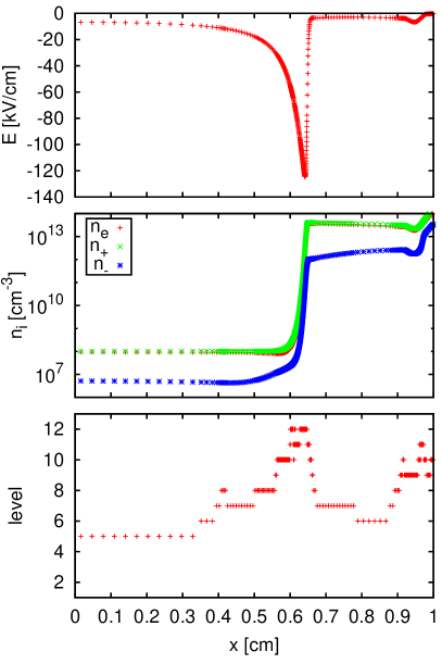
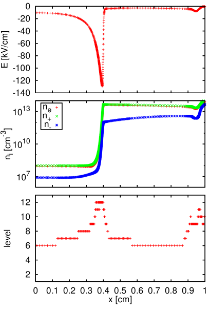
Two instances of the discharge propagation are shown in Figure 5, for $12$ nested grids equivalent to $4096$ cells on the finest grid, $L=12$, and for accuracy tolerances of $\eta_{\mathcal{T}}=\eta_{\rm split}=\eta_{\rm MR}=10^{-4}$; the spatial refinement takes place only where it is required. Fine tolerances were chosen in all cases for the solvers, $\eta_{\rm Radau5}=\eta_{\rm ROCK4}=10^{-7}$, to guarantee accurate integrations. For all the simulation cases, the detail in each cell is taken as the maximum of the details computed according to (27) for each variable, where the prediction operator is a polynomial interpolation of degree $2$, performed on normalized $\log{\bf u}$ of the density variables in order to properly discriminate the streamer heads from the highly ionized plasma channel; this logarithmic scale guarantees a correct spatial representation of the phenomenon as seen in Figure 5 for the density profiles.

In order to perform an analysis of the numerical results, we define the reference solution as a fine resolution with the $\mathcal{T}_{2}$ scheme that considers a fixed decoupling time step, $\Delta t=10^{-14}\,$s and a uniform grid of $4096$ cells. For this reference solution, the memory requirements are acceptable and the simulation is still feasible, but it requires about 14 days of real simulation time on an AMD Opteron 6136 Processor cluster, while running the electric field computation in parallel on 16 CPU cores. In this case, the computation of the electric field, based on a direct integration of individual contributions of the charged cylinders, represents 80% of total CPU time per time step (about $3.2\,$s).

Figure 6: Normalized $L^{2}$ errors between the reference and the $\mathcal{T}_{1}$ (first order) and $\mathcal{T}_{2}$ (second order) solutions for several decoupling time steps $\Delta t$ on a uniform grid of 4096 cells. Top: electron (left) and positive ions (right); and bottom: negative ions.

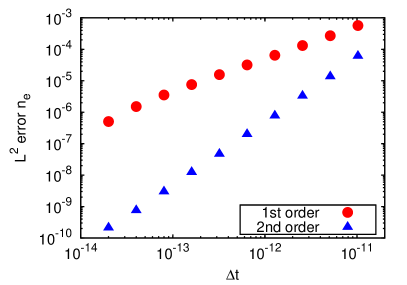
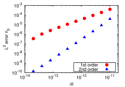
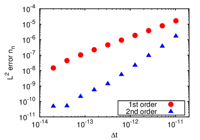
First of all, we must verify the previous order estimates for the $\mathcal{T}_{1}$ and $\mathcal{T}_{2}$ schemes given in Section 3.1. We consider as initial condition the reference solution at $t=10\,$ns. In order to only evaluate errors coming from the decoupling techniques, $\mathcal{T}_{1}$ and $\mathcal{T}_{2}$, we consider a fine splitting time step, $\Delta t_{\rm s}=10^{-14}\,$s, to solve the drift-diffusion problem (1) and a uniform grid; then, we solve (5) with both schemes for several decoupling time steps $\Delta t_{i}$, and calculate the normalized $L^{2}$ error between the first/second order and reference solutions after time $t=2^{10}\Delta t_{\rm s}=1.024\times 10^{-11}\,$s. Figure 6 shows results with $\Delta t_{i}=2^{i}\Delta t_{\rm s}$, where $i\in[1,10]$, which clearly verify first and second order in time for the $\mathcal{T}_{1}$ and $\mathcal{T}_{2}$ schemes, respectively, and prove important gains in accuracy for same time steps. For instance, for $\Delta t\leq 10^{-12}\,$s the second order scheme provides solutions with $L^{2}$ errors at least $100$ times lower than those obtained with the first order method.

Figure 7: Time evolution of the normalized $L^{2}$ errors between the reference and adapted solutions with $\eta=\eta_{\mathcal{T}}=\eta_{\rm split}=\eta_{\rm MR}=10^{-4}$, $10^{-3}$, and $10^{-2},$ and 4096 cells corresponding to the finest discretization. Top: electron (left) and positive ions (right); and bottom: negative ions.

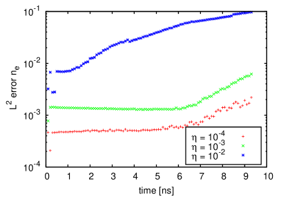
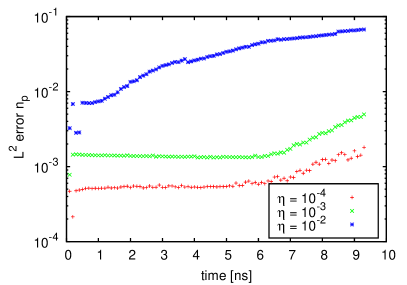
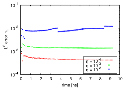
Figure 7 shows the time evolution of the normalized $L^{2}$ error for each variable between the time-space adapted and reference solutions for several tolerances, $\eta_{\mathcal{T}}=\eta_{\rm split}=\eta_{\rm MR}=10^{-4}$, $10^{-3}$, and $10^{-2}$. These are rather approximations of the error since the reference and adapted solutions are not evaluated exactly at the same time, and therefore, they are often slightly shifted of about $\sim$$10^{-14}-10^{-13}$s. In these tests, the decoupling time steps $\Delta t$ were limited by the dielectric relaxation time step, $\Delta t_{DR}$, after noticing an important amount of rejections of computed time steps according to (18), whenever $\Delta t\gtrsim$$1.5\times\Delta t_{DR}$. Otherwise, $\Delta t$ is dynamically chosen in order to locally satisfy the required accuracy $\eta_{\mathcal{T}}$, but it does not show important variations considering the self-similar propagating phenomenon.

Figure 8: Top: adapted grids (left) and electric fields (right) at $t=8\,$ns with 4096 cells corresponding to the finest discretization, and $\eta=\eta_{\mathcal{T}}=\eta_{\rm split}=\eta_{\rm MR}=10^{-4}$, $10^{-3}$, and $10^{-2}$. Bottom: zoom on the electron distributions (left) and the electric field (right) with the same parameters, and the reference solution.

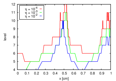
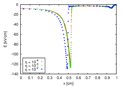
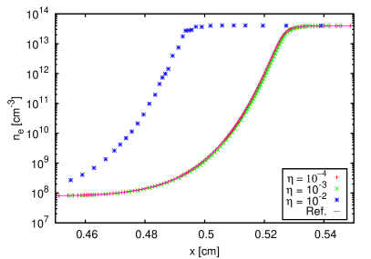
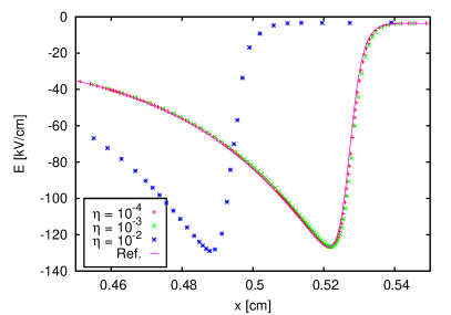
In Figure 8, we can see the corresponding adapted grid to each previous configuration with different tolerances. The representation of the electric field and the densities shows that for $\eta_{\mathcal{T}}=\eta_{\rm split}=\eta_{\rm MR}=10^{-2}$, the streamer front propagates faster than in the reference case, with a slightly higher peak of the electric field in the front. On the other hand, for $\eta_{\mathcal{T}}=\eta_{\rm split}=\eta_{\rm MR}\leq 10^{-3}$, we observe a quite good agreement between the adapted and reference resolutions.

Figure 9: Adapted grids (left) and electric fields (right) at $t=8\,$ns, for several finest spatial discretization $L=10$, 11 and 12, $\eta_{\mathcal{T}}=\eta_{\rm split}=\eta_{\rm MR}=10^{-4}$, and the reference solution.

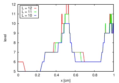
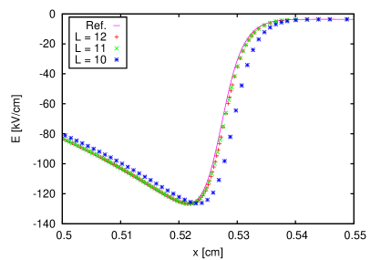
We consider now an accurate enough resolution with $\eta_{\mathcal{T}}=\eta_{\rm split}=\eta_{\rm MR}=10^{-4}$ and investigate the influence of the number of grids, that is, the finest spatial discretization at level $L$ that should be taken into account. Figure 9 shows the adapted grids for $L=10$, $11$ and $12$, respectively equivalent to $1024$, $2048$ and $4096$ cells in the finest grid; and a close-up of the corresponding electric fields in the discharge head at $t=8\,$ns. We see that for this level of tolerances, the streamer front propagates slightly slower than the reference case for $L=10$, whereas $L=11$ gives already good resolutions compared with the reference solution and with $L=12$. In particular, higher values of $L$ would need lower tolerances in order to retain regions at the finest level; this is already the case for $L=13$ (equivalent to $8192$ cells). Therefore, $L=11$ with $2048$ cells at the finest level seems to be an appropriate choice for this level of accuracy.

Table 1 summarizes the number of cells in the adapted grid ($\#AG$) at time $t=8$ns, and the corresponding data compression ($DC$) defined as the percentage of active cells with respect to the equivalent number of cells for the finest discretization, in this case $2048$ for $L=11$. For this propagating case, the data compression remains of the same order during the time simulation interval. The CPU computing times correspond to a time domain of study of $t\in[0,10]\,$ns computed by one sole CPU core. If we consider for example total computing time for $L=11$ and tolerances $\eta_{\mathcal{T}}=\eta_{\rm split}=\eta_{\rm MR}=10^{-4}$, it is $\sim$$44$ times less expensive with respect to a resolution on a uniform grid with $2048$ cells and $\eta_{\mathcal{T}}=\eta_{\rm split}=10^{-4}$ (CPU time of $8552\,$s). This is quite reasonable, taking into account that the computing time for the electric field resolution is proportional to at least $\mathcal{O}(N^{2})$ for $N$ computing cells, after (32).

Table 1: Number of cells in the adapted grid ($\#AG$) and data compression ($DC$) at time $t=8$ns, CPU computing time for $t\in[0,10]$ ns, $L=11$, and several tolerances $\eta=\eta_{\mathcal{T}}=\eta_{\rm split}=\eta_{\rm MR}$.

$\eta$ $\#AG$ $DC$% CPU(s) $10^{-6}$ $724$ $35.35$ $1360$ $10^{-5}$ $421$ $20.56$ $\phantom{0}517$ $10^{-4}$ $263$ $12.84$ $\phantom{0}193$ $10^{-3}$ $138$ $\phantom{0}6.74$ $\phantom{00}66$ $10^{-2}$ $\phantom{0}70$ $\phantom{0}3.42$ $\phantom{00}24$

In conclusion, in this section we have shown that the numerical strategy developed can be efficiently applied to simulate the propagation of highly nonlinear ionizing waves as streamer discharges. An important reduction of computing time results from significant data compression with still accurate resolutions. In addition, this study allows to properly tune the various simulation parameters in order to guarantee a fine resolution of more complex configurations, based on the time-space accuracy control capabilities of the method.

4.2 Simulation of multi-pulsed discharges

In this section, we analyze the performance of the proposed numerical strategy on the simulation of nanosecond repetitively pulsed discharges [6, 60]. The applied voltage profile for this type of discharges is a high voltage pulse followed by a zero voltage relaxation phase. The typical pulse duration is $\sim$$10^{-8}\,$s, while the relaxation phase takes over $\sim$$10^{-4}\,$s. The detailed experimental study of these discharges in air has shown that the cumulative effect of repeated pulsing achieves a steady-state behavior [60]. In the following illustrations, we choose a pulse duration of $T_{\rm p}=15\,$ns, which is approximately equal to the time that is needed for the discharge to cross the inter-electrode gap. The rise time considers the time needed to go from zero to the maximum voltage and it is set to $T_{\rm r}=2\,$ns. The pulse repetition period is set to $T_{\rm P}=10^{-4}\,$s, equal to $10\,$kHz of repetition frequency, a typical value used in experiments [6]. We model the voltage pulse $P$ by using sigmoid functions

$$P(t,s,r,p)=1-\sigma(-t,-s,r)-\sigma(t,s+p,r),$$ (34)

with

$$\sigma(t,s,r)=\frac{1}{1+\exp(-8(t-s)/r)},$$ (35)

for time $t$, where $s$ indicates when the pulse starts; $r$ is the rise time; and $p$ is the pulse duration; $t$, $s$, $r$, $p\in[0,T_{\rm P}]$. With a maximum applied voltage $V_{\rm max}$, the applied voltage $V(t)$ is computed by

$$V(t)=V_{\rm max}\cdot P\left(t-\left\lfloor\frac{t}{T_{\rm P}}\right\rfloor\cdot T_{\rm P},T_{\rm r},T_{\rm r},T_{\rm p}\right).$$ (36)

In repetitively pulse discharges at atmospheric pressure and $300\,$K, as discussed in [46, 47], electrons attach rapidly to $O_{2}$ molecules during the interpulse to form negative ions (characteristic time scale of $20\,$ns). Then, the rate of the plasma decay is determined by ion-ion recombination [45, 46, 47]. When the next voltage pulse is applied, electrons are detached with a rate taken from [44]. Therefore, as initial condition we assume a distribution similar to the end of the interpulse phase with a homogeneous preionization consisting of positive and negative ions with a density of $10^{9}\,$cm^-3. For electrons, we consider a low homogeneous background of $10^{1}\,$cm^-3. This small amount of electrons as initial condition has a negligible influence on the results.

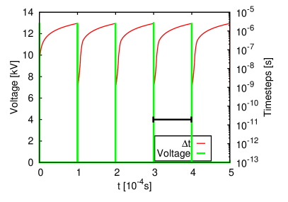
We set the tolerances to $\eta_{\mathcal{T}}=\eta_{\rm split}=\eta_{\rm MR}=10^{-4}$ and consider $L=11$ grid levels, equivalent to $2048$ cells in the finest grid. As in the previous configuration, homogeneous Neumann boundary conditions were considered for the drift-diffusion equations. Figure 10 shows the time evolution of the decoupling time steps and the applied voltage for the first six pulses, even though simulation was performed for 100 pulses, that is $t\in[0,10^{-2}]\,$s. This simulation took over $8$h$44$m while running the electric field computation in parallel on $6$ CPU cores of the same AMD Opteron 6136 Processor cluster; this gives an average of $5.24$ minutes per pulse period. Figure 10 shows also the fourth pulse for which the steady-state of the periodic phenomenon was already reached and almost the same numerical performance is reproduced during the rest of computations. The time steps are about $\sim$$10^{-11}\,$s during pulses, then increase from $\sim$$10^{-12}\,$s up to about $\sim$$10^{-6}\,$s during a period $\sim$$6000$ times longer, for which standard stability constraints are widely overcome according to the required accuracy tolerance. Solving this problem for such different scales with a constant time step is out of question and even a standard strategy that considers the minimum of all time scales would limit considerably the efficiency of the method as it is shown in the representation. In this particular case, the dielectric relaxation is the governing time scale during the discharge as in the previous case with constant applied voltage, whereas the post-discharge phase is alternatively ruled by diffusive or convective CFL, or by ionization time scale, with all security factors and CFL conditions set to one in Figure 10.

Figure 10: Time evolution of the applied voltage and the decoupling time steps $\Delta t$ for a multi-pulse simulation for the first 6 pulses (left) and for the 4th one (right) with its subsequent relaxation. Rejected time steps are marked with black crosses, while the minimum time scale corresponds to the blue line.

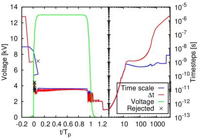
The computation is initialized with a time step included in the pulse duration. Nevertheless, after each relaxation phase, since the new time step is computed based on the previous one according to (18), this new time step will surely skip the next pulse. In order to avoid this, each time we get into a new period, that is when $\lfloor t/T_{\rm P}\rfloor$ changes, we initialize the time step with $\Delta t=0.5T_{\rm r}=1\,$ns. This time step is obviously rejected as seen in Figure 10, as well as the next ones, until we are able to retrieve the right dynamics of the phenomenon for the required accuracy tolerance. No other intervention is needed neither for modeling parameters nor for numerical solvers in order to automatically adapt the time step needed to describe the various time scales of the phenomenon within a prescribed accuracy.

Figure 11 represents the time evolution of the data compression which ranges from $\sim$$2\%$ up to $\sim$$16\%$ during each pulse period. Regarding only the electric field resolution with the same time integration strategy, a grid adaptation technique involves resolutions $\sim$$39$ to $\sim$$2500$ times faster, based on a really rough estimate for $\mathcal{O}(N^{2})$ operations.

Figure 11: Time evolution of the data compression for a multi-pulse simulation for the first six pulses (left) and for the fourth one (right) with its subsequent relaxation.

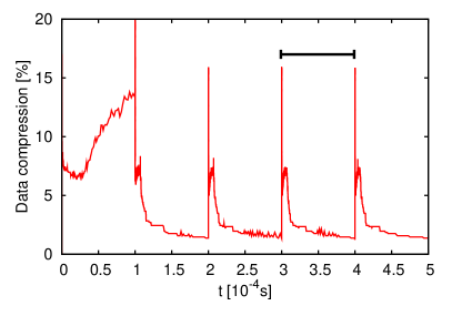
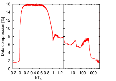
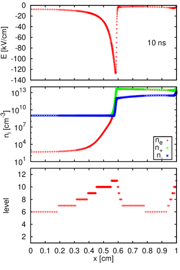
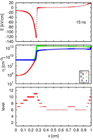
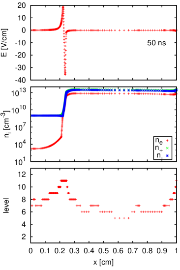
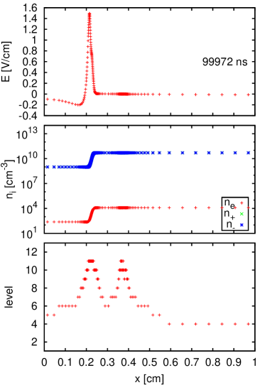
Figure 12 presents the discharge dynamics for the first period. First, we observe at $t=10\,$ns after the beginning of the pulse, the propagation of a positive streamer in the gap. In Section 4.1, a preionization of positive ions and electrons was used to ensure the positive streamer propagation. In this section, seed electrons ahead of the streamer front are created as the front propagates by detachment of negative ions initially present. We note that at $15\,$ns, which corresponds to almost the end of the plateau before the decrease of the applied voltage, the discharge has crossed $\sim$$0.75\,$cm of the $1\,$cm gap. As a consequence, during the voltage decrease and at the beginning of the relaxation phase where the applied voltage is zero, there is a remaining space charge and steep gradients of charged species densities in the gap. Then for $t=50\,$ns, Figure 12 shows that the electric field in the discharge is almost equal to zero except in a small area where steep gradients of the electric field are observed but with peak values of only $30\,$V/cm. We have checked that this area corresponds to the location of the streamer head at the end of its propagation as it is seen in the representation. We note that in the post-discharge, electrons are attaching and then at $t=50\,$ns, the density of positive ions is almost equal to the density of negative ions in the whole gap. At $t=99972\,$ns, the densities of charged species have significantly decreased due to charged species recombination. However, it is interesting to note that the location of the previous streamer head can still be observed at the same location as at $t=50\,$ns, but with much smaller gradients of charged species densities and a very small electric field. This final state is the initial condition of the second pulse with a non-uniform axial preionization with positive and negative ions and a much smaller density of electrons.

Figure 12: First period of pulsed discharges. Top: propagation of the discharge in the domain at $t=10\,$ns after the beginning of the pulse (left); and at $t=15\,$ns (right). Bottom: relaxation on the short time scale $t=50\,$ns; and end of the relaxation phase after $t=99972\,$ns (right).

Figure 13: Steady-state of pulsed discharges (last period). Top: propagation of the discharge in the domain at $t=9900010\,$ns after the beginning of the pulse (left); and at $t=9900015\,$ns (right). Bottom: relaxation on short time scale $t=9900050\,$ns; and end of the relaxation phase $t=9999998\,$ns (right).

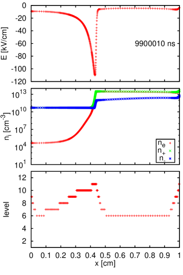
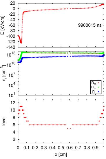
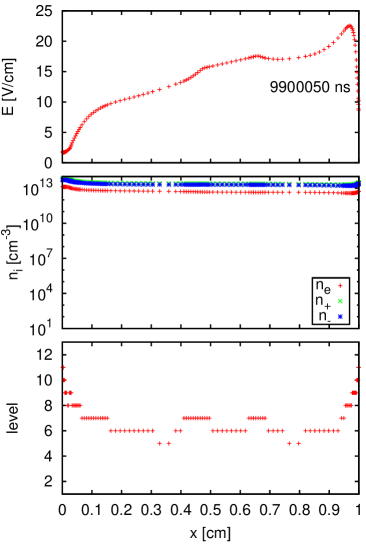
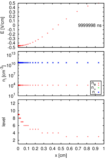
After a few repetitive pulses, we have observed that the discharge dynamics reached a steady-state behavior as observed in the experiments. To show the characteristics of the discharge when the steady-state is reached, Figure 13 shows the discharge dynamics of the 100th period. The sequence of images is the same as in Figure 12. At the end of the 99th pulse, we have observed that the axial distribution of charged species in the gap is uniform and that the level of preionization is $5\times 10^{10}\,$cm^-3 positive and negative ions and $10^{4}\,$cm^-3 electrons. We note that $10\,$ns after the beginning of the 100th pulse the propagation of the discharge is faster than for the first pulse. This faster propagation is mostly due to the higher preionization level of positive and negative ions in the gap in comparison of the first voltage pulse. We observe that for the 100th pulse, $15\,$ns after the beginning of the pulse the discharge has almost completely crossed the inter-electrode gap and then during the relaxation phase, there is no remaining space charge in the whole gap. Consequently, $50\,$ns after the beginning of the 100th pulse, axial distributions of all charged species are uniform. As already observed for the first pulse, at $50\,$ns after the beginning of the voltage pulse most electrons have attached and then, the density of positive ions is almost equal to the density of negative ions in the whole gap. We see that the corresponding electric field distribution is not uniform at $50\,$ns, but no steep gradients are observed as for the first voltage pulse. At $t=9999998\,$ns, that is to say at the end of the 100th period, we note that a very low electric field is obtained in the gap. An axially uniform distribution of charges is obtained with $5\times 10^{10}\,$cm^-3 for positive and negative ions and $10^{4}\,$cm^-3 for electrons, which was the initial condition of the 100th pulse. This demonstrates the existence of a steady-state behavior of these nanosecond repetitively pulsed discharges.

5 Conclusions

The present work proposes a new numerical strategy for multi-scale streamer simulations. It is based on an adaptive second order time integration strategy that allows to discriminate time scales-related features of the phenomena, given a required level of accuracy of computations. Compared with a standard procedure for which accuracy is guaranteed by considering time steps of the order of the fastest scale, the control error approach implies on the one hand, an effective accurate resolution independent of the fastest physical time scale, and on the other hand, an important improvement of computational efficiency whenever the required time steps go beyond standard stability constraints. The latter is a direct consequence of the self-adaptive time step strategy for the resolution of the drift-diffusion equations which considers splitting time steps not limited by stability constraints for reaction, diffusion and convection phenomena. So far, the global decoupling time steps are limited by the dielectric relaxation stability constraint but with a second order accuracy. Nevertheless, we have also demonstrated that the decoupling time steps are rather chosen based on an accuracy criterion. Besides, if a technique such as a semi-implicit approach is implemented, the same ideas of the proposed adaptive strategy remain valid.

An adaptive multiresolution technique was also proposed in order to provide error control of the spatial adapted representation. The numerical results have proven a natural coupling between time and space accuracy requirements and how the set of time-space accuracy tolerances tunes the precise description of the overall time-space multi-scale phenomenon. As a consequence, the numerical results for multi-pulsed discharge configurations prove that this kind of multi-scale phenomena, previously out of reach, can be successfully simulated with conventional computing resources by this time-space adaptive strategy. And they also show that a consistent physical description is achieved for a broad spectrum of space and time scales as well as different physical scenarios.

In this work, we focused on a 1.5D model in order to evaluate the numerical performance of the strategy. However, the dimension of the problem will only have an influence on the computational efficiency measurements but not on any space-time accuracy or stability aspects. At this stage of development, the same numerical strategy can be coupled with a multi-dimensional Poisson’s equation solver, even for adapted grid configurations as developed recently in [23, 4, 20]. Finally, an important amount of work is still in progress concerning programming features such as data structures, optimized routines and parallelization strategies. On the other hand, numerical analysis of theoretical aspects is also underway to extend and further improve the proposed numerical strategy. These issues constitute particular topics of our current research.

References

- [1] E. M. van Veldhuizen (Ed.), Electrical Discharges for Environmental Purposes: Fundamentals and Applications, Nova Science, New York, 2000.
- [2] A. Fridman, A. Chirokov, A. Gutsol, Non-thermal atmospheric pressure discharges, J. Phys. D: Appl. Phys. 38 (2005) R1–R24.
- [3] P. A. Vitello, B. M. Penetrante, J. N. Bardsley, Simulation of negative-streamer dynamics in nitrogen, Phys. Rev. E 49 (1994) 5574–5598.
- [4] T. Unfer, J.-P. Boeuf, F. Rogier, F. Thivet, Multi-scale gas discharge simulations using asynchronous adaptive mesh refinement, Computer Physics Communications 181 (2) (2010) 247 – 258.
- [5] U. Ebert, F. Brau, G. Derks, W. Hundsdorfer, C.-Y. Kao, C. Li, A. Luque, B. Meulenbroek, S. Nijdam, V. Ratushnaya, L. Schäfer, S. Tanveer, Multiple scales in streamer discharges, with an emphasis on moving boundary approximations, Nonlinearity 24 (1) (2011) C1–C26.
- [6] G. Pilla, D. Galley, D. Lacoste, F. Lacas, D. Veynante, C. Laux, Stabilization of a turbulent premixed flame using a nanosecond repetitively pulsed plasma, IEEE Trans. Plasma Sci. 34 (6, Part 1) (2006) 2471–2477. doi:10.1109/TPS.2006.886081.
- [7] D. F. Opaits, M. N. Shneider, R. B. Miles, A. V. Likhanskii, S. O. Macheret, Surface charge in dielectric barrier discharge plasma actuators, Phys. Plasmas 15 (7) (2008) 073505. doi:10.1063/1.2955767.
- [8] A. Davies, F. Jones, C. Evans, Electrical breakdown of gases - Spatio-temporal growth of ionization in fields distorted by space charge, Proc. Royal Soc. London S. A-Math. and Phys. Scien. 281 (1385) (1964) 164–183.
- [9] A. Davies, C. Davies, C. Evans, Computer simulation of rapidly developing gaseous discharges, Proc. of the Institution of Electrical Engineers-London 118 (6) (1971) 816–823.
- [10] I. Abbas, P. Bayle, A critical analysis of ionizing wave-propagation mechanisms in breakdown, J. Phys. D: Appl. Phys. 13 (6) (1980) 1055–1068.
- [11] R. Morrow, Theory of negative corona in oxygen, Phys. Rev. A 32 (3) (1985) 1799–1809.
- [12] S. K. Dhali, P. F. Williams, Two-dimensional studies of streamers in gases, J. Appl. Phys. 62 (1987) 4696–4707.
- [13] N. Y. Babaeva, G. V. Naidis, Dynamics of positive and negative streamers in air in weak uniform electric fields, IEEE Trans. Plasma Sci. 25 (1997) 375–379.
- [14] A. A. Kulikovsky, The role of photoionization in positive streamer dynamics, J. Phys. D: Appl. Phys. 33 (2000) 1514–1524.
- [15] S. V. Pancheshnyi, S. M. Starikovskaia, A. Y. Starikovskii, Role of photoionization processes in propagation of cathode-directed streamer, J. Phys. D: Appl. Phys. 34 (2001) 105–115.
- [16] M. Arrayás, U. Ebert, W. Hundsdorfer, Spontaneous branching of anode-directed streamers between planar electrodes, Phys. Rev. Lett. 88 (2002) 174502(R).
- [17] S. Celestin, Z. Bonaventura, B. Zeghondy, A. Bourdon, P. Segur, The use of the ghost fluid method for Poisson’s equation to simulate streamer propagation in point-to-plane and point-to-point geometries, J. Phys. D: Appl. Phys. 42 (6) (2009) 065203. doi:{10.1088/0022-3727/42/6/065203}.
- [18] A. Bourdon, Z. Bonaventura, S. Celestin, Influence of the pre-ionization background and simulation of the optical emission of a streamer discharge in preheated air at atmospheric pressure between two point electrodes, Plasma Sources Sci. Technol. 19 (3) (2010) 034012. doi:{10.1088/0963-0252/19/3/034012}.
- [19] D. S. Nikandrov, R. R. Arslanbekov, V. I. Kolobov, Streamer simulations with dynamically adaptive cartesian mesh, IEEE Trans. Plasma Sci. 36 (4) (2008) 932–933.
- [20] S. Pancheshnyi, P. Segur, J. Capeillere, A. Bourdon, Numerical simulation of filamentary discharges with parallel adaptive mesh refinement, J. Comp. Phys. 227 (13) (2008) 6574–6590.
- [21] A. Luque, U. Ebert, W. Hundsdorfer, Interaction of streamer discharges in air and other oxygen-nitrogen mixtures, Phys. Rev. Lett. 101 (7) (2008) 075005. doi:10.1103/PhysRevLett.101.075005.
- [22] L. Papageorgiou, A. C. Metaxas, G. E. Georghiou, Three-dimensional numerical modelling of gas discharges at atmospheric pressure incorporating photoionization phenomena, J. Phys. D: Appl. Phys. 44 (4) (2011) 045203.
- [23] C. Montijn, W. Hundsdorfer, U. Ebert, An adaptive grid refinement strategy for the simulation of negative streamers, J. Comput. Phys. 219 (2) (2006) 801–835.
- [24] A. Bourdon, V. P. Pasko, N. Y. Liu, S. Celestin, P. Segur, E. Marode, Efficient models for photoionization produced by non-thermal gas discharges in air based on radiative transfer and the Helmholtz equations, Plasma Sources Sci. Technol. 16 (3) (2007) 656–678. doi:{10.1088/0963-0252/16/3/026}.
- [25] P. L. G. Ventzek, T. J. Sommerer, R. J. Hoekstra, M. J. Kushner, Two-dimensional hybrid model of inductively coupled plasma sources for etching, Appl. Phys. Lett. 63 (5) (1993) 605 – 607.
- [26] P. Colella, M. R. Dorr, D. D. Wake, A conservative finite difference method for the numerical solution of plasma fluid equations, J. Comput. Phys. 149 (1) (1999) 168 – 193.
- [27] G. J. M. Hagelaar, G. M. W. Kroesen, Speeding up fluid models for gas discharges by implicit treatment of the electron energy source term, J. Comp. Phys. 159 (1) (2000) 1–12.
- [28] H. Karimabadi, J. Driscoll, Y. Omelchenko, N. Omidi, A new asynchronous methodology for modeling of physical systems: breaking the curse of courant condition, J. Comp. Phys. 205 (2) (2005) 755 – 775.
- [29] Y. Omelchenko, H. Karimabadi, Self-adaptive time integration of flux-conservative equations with sources, J. Comp. Phys. 216 (1) (2006) 179 – 194.
- [30] T. Unfer, J.-P. Boeuf, F. Rogier, F. Thivet, An asynchronous scheme with local time stepping for multi-scale transport problems: Application to gas discharges, J. Comp. Phys. 227 (2) (2007) 898 – 918.
- [31] F. Coquel, Q. L. Nguyen, M. Postel, Q. H. Tran, Local time stepping for implicit-explicit methods on time varying grids, in: K. Kunisch, G. Of, O. Steinbach (Eds.), Numerical Mathematics and Advanced Applications, Springer Berlin Heidelberg, 2008, pp. 257–264.
- [32] M. O. Domingues, S. M. Gomes, O. Roussel, K. Schneider, An adaptive multiresolution scheme with local time stepping for evolutionary PDEs, J. Comp. Phys. 227 (8) (2008) 3758 – 3780.
- [33] F. Coquel, Q. L. Nguyen, M. Postel, Q. H. Tran, Local time stepping applied to implicit-explicit methods for hyperbolic systems, Multiscale Model. Simul. 8 (2) (2010) 540–570.
- [34] M. Duarte, M. Massot, S. Descombes, C. Tenaud, T. Dumont, V. Louvet, F. Laurent, New resolution strategy for multi-scale reaction waves using time operator splitting, space adaptive multiresolution and dedicated high order implicit/explicit time integrators, Submitted to SIAM J. Sci. Comput. (2011) available on HAL (http://hal.archives–ouvertes.fr/hal–00457731).
- [35] T. Dumont, M. Duarte, S. Descombes, M.-A. Dronne, M. Massot, V. Louvet, Simulation of human ischemic stroke in realistic 3D geometry: A numerical strategy, Submitted to Bulletin of Math. Biology (2011) available on HAL (http://hal.archives–ouvertes.fr/hal–00546223).
- [36] S. Descombes, M. Duarte, T. Dumont, V. Louvet, M. Massot, Adaptive time splitting method for multi-scale evolutionary PDEs, Accepted to Confluentes Mathematici (2011) available on HAL (http://hal.archives–ouvertes.fr/hal–00587036).
- [37] M. Duarte, M. Massot, S. Descombes, T. Dumont, Adaptive time-space algorithms for the simulation of multi-scale reaction waves, in: Finite Volumes for Complex Applications VI - Problems & Perspectives, Springer Proceedings in Mathematics Volume 4, 2011, pp. 379–387.
- [38] A. Harten, Multiresolution algorithms for the numerical solution of hyperbolic conservation laws, Comm. Pure and Applied Math. 48 (1995) 1305–1342.
- [39] A. Cohen, S. Kaber, S. Müller, M. Postel, Fully adaptive multiresolution finite volume schemes for conservation laws, Mathematics of Comp. 72 (2003) 183–225.
- [40] D. Bessieres, J. Paillol, A. Bourdon, P. Segur, E. Marode, A new one-dimensional moving mesh method applied to the simulation of streamer discharges, J. Phys. D: Appl. Phys. 40 (21) (2007) 6559–6570. doi:{10.1088/0022-3727/40/21/016}.
- [41] N. Y. Babaeva, G. V. Naidis, Two-dimensional modelling of positive streamer dynamics in non-uniform electric fields in air, J. Phys. D: Appl. Phys. 29 (1996) 2423–2431.
- [42] A. A. Kulikovsky, Positive streamer between parallel plate electrodes in atmospheric pressure air, J. Phys. D: Appl. Phys. 30 (1997) 441–450.
- [43] R. Morrow, J. J. Lowke, Streamer propagation in air, J. Phys. D: Appl. Phys. 30 (1997) 614–627.
- [44] M. S. Benilov, G. V. Naidis, Modelling of low-current discharges in atmospheric-pressure air taking account of non-equilibrium effects, J. Phys. D: Appl. Phys. 36 (15) (2003) 1834–1841.
- [45] I. A. Kossyi, A. Y. Kostinsky, A. A. Matveyev, V. P. Silakov, Kinetic scheme of the non-equilibrium discharge in nitrogen-oxygen mixtures, Plasma Sources Sci. Technol. 1 (3) (1992) 207–220.
- [46] S. V. Pancheshnyi, Role of electronegative gas admixtures in streamer start, propagation and branching phenomena, Plasma Sources Sci. Technol. 14 (4) (2005) 645–653.
- [47] G. Wormeester, S. Pancheshnyi, A. Luque, S. Nijdam, U. Ebert, Probing photo-ionization: simulations of positive streamers in varying N2:O2 mixtures, J. Phys. D: Appl. Phys. 43 (50) (2010) 505201.
- [48] S. Celestin, Study of the streamer dynamics in air at atmospheric pressure, PhD thesis, Ecole Centrale Paris, France, 2008.
- [49] G. Strang, On the construction and comparison of difference schemes, SIAM J. Numer. Anal. 5 (1968) 506–517.
- [50] S. Descombes, M. Massot, Operator splitting for nonlinear reaction-diffusion systems with an entropic structure: Singular perturbation and order reduction, Numer. Math. 97 (4) (2004) 667–698.
- [51] E. Hairer, G. Wanner, Solving ordinary differential equations II, 2nd Edition, Springer-Verlag, Berlin, 1996, Stiff and differential-algebraic problems.
- [52] A. Abdulle, Fourth order Chebyshev methods with recurrence relation, SIAM J. Sci. Comput. 23 (2002) 2041–2054.
- [53] V. Daru, C. Tenaud, High order one-step monotonicity-preserving schemes for unsteady compressible flow calculations, J. Comput. Phys. 193 (2) (2004) 563 – 594.
- [54] M. Duarte, M. Massot, S. Descombes, C. Tenaud, T. Dumont, V. Louvet, F. Laurent, New resolution strategy for multi-scale reaction waves using time operator splitting and space adaptive multiresolution: Application to human ischemic stroke, ESAIM Proceedings (2011) available on HAL (http://hal.archives–ouvertes.fr/hal–00590812).
- [55] A. Cohen, Wavelet methods in numerical analysis, Vol. 7, Elsevier, Amsterdam, 2000.
- [56] S. Müller, Adaptive multiscale schemes for conservation laws, Vol. 27, Springer-Verlag, 2003.
- [57] C. F. Eyring, S. S. Mackeown, R. A. Millikan, Fields currents from points, Phys. Rev. 31 (5) (1928) 900–909.
- [58] J. D. Jackson, Classical Electrodynamics, 3rd Edition, John Wiley and Sons, Inc., 1999, page 26, equation (1.5).
- [59] A. A. Kulikovsky, Positive streamer in a weak field in air: A moving avalanche-to-streamer transition, Phys. Rev. E 57 (6) (1998) 7066–7074.
- [60] D. Z. Pai, D. A. Lacoste, C. O. Laux, Transitions between corona, glow, and spark regimes of nanosecond repetitively pulsed discharges in air at atmospheric pressure, J. Appl. Phys. 107 (9) (2010) 093303. doi:10.1063/1.3309758.