Outage Probability in $\eta$-$\mu$/$\eta$-$\mu$ Interference-limited Scenarios

Abstract

In this paper exact closed-form expressions are derived for the outage probability (OP) in scenarios where both the signal of interest (SOI) and the interfering signals experience $\eta$-$\mu$ fading and the background noise can be neglected. With the only assumption that the $\mu$ parameter is a positive integer number for the interfering signals, the derived expressions are given in elementary terms for maximal ratio combining (MRC) with independent branches. The analysis is also valid when the $\mu$ parameters of the pre-combining SOI power envelopes are positive integer or half-integer numbers and the SOI is formed at the receiver from spatially correlated MRC.

I Introduction

The $\eta$-$\mu$ fading distribution has been proposed to model a general non-line-of-sight (NLOS) propagation scenario. By two shape parameters $\eta$ and $\mu$, this model includes some classical fading distributions as particular cases, e.g. Nakagami-$q$ (Hoyt), one-sided Gaussian, Rayleigh and Nakagami-$m$. The fitting of the $\eta$-$\mu$ distribution to experimental data is better than that achieved by the classical distributions previously mentioned. A detailed description of the $\eta$-$\mu$ fading model can be found in [1].

This paper focuses on outage probability (OP) analysis for wireless communications systems where both the signal of interest (SOI) and the cochannel interference (CCI) signals experience $\eta$-$\mu$ fading and the background noise can be neglected. The OP analysis for $\eta$-$\mu$ fading channels in which only the background noise is present was recently published in [2]. A detailed account of OP analysis for interference-limited systems can be found in [3, chapter 10] and references therein. Specifically, in [3, eq. 10.17] a closed-form expression is derived for the OP in the Nakagami-$m$/Nakagami-$m$ interference-limited scenario assuming independent and identically distributed (i.i.d) receive maximal ratio combining (MRC) for the SOI, i.i.d interfering signals, and certain restrictions for the values of the Nakagami-$m$ parameters of both the SOI and the interferers. In fact, this expression for the Nakagami-$m$/Nakagami-$m$ scenario includes, as particular cases, several classical results derived in literature [4]-[7]. More recently, a further generalization for the Nakagami-$m$/Nakagami-$m$ interference-limited scenario was presented in [8], where a closed-form expression was derived in [8, eq. 18] for i.i.d MRC with the only restriction that the product of the $m$ parameter and the number of MRC branches for the SOI is a positive integer number. However, to the best of the author’s knowledge, no closed-form results in elementary terms for the $\eta$-$\mu$/$\eta$-$\mu$ interference-limited scenario, which consequently generalize current results for the Nakagami-$m$/Nakagami-$m$ scenario, are found in literature.

In this paper, we derive exact closed-form expressions for the OP of the $\eta$-$\mu$/$\eta$-$\mu$ interference-limited scenario in elementary terms, with the only assumption that the $\mu$ parameter is a positive integer number for the interfering signals. Such analysis is further extended to scenarios in which the SOI is formed from spatially correlated MRC. In connection with the Nakagami-$m$/Nakagami-$m$ scenario, the derived expressions complement [3, eq. 10.17] and [8, eq. 18] as long as they are valid if real values of $m$ are assumed for the pre-combining SOI power envelopes or if the SOI is formed from spatially correlated MRC. In addition, the presented OP analysis includes other interesting scenarios, e.g. the $\eta$-$\mu$/Rayleigh interference-limited scenario with no assumptions on the SOI and the interferers parameters.

The remainder of this paper is organized as follows. In Section II the key statistical results for $\eta$-$\mu$/$\eta$-$\mu$ random variables (RVs) are derived. The OP analysis is discussed in Section III and the numerical results in Section IV. Finally, some conclusions are given in Section V.

II Distribution of the Quotient of Sums of Squared $\eta$-$\mu$ RVs

The fundamental results of this paper are expressed in statistical terms in the next Lemma and its Corollary. Along this paper all $\eta$-$\mu$ RVs are assumed to be defined by format 1, i.e. $\eta>0$ and $\mu>0$. For details on $\eta$-$\mu$ RVs, the reader should refer to [1].

Lemma 1

Let $\{X_{n}\}_{n=1}^{N}$ and $\{Y_{k}\}_{k=1}^{K}$ be $N+K$ mutually independent squared $\eta$-$\mu$ RVs with sets of parameters, defined according to format 1, given by $\mathcal{S}_{X}\equiv\{\Omega_{X_{n}},\eta_{X_{n}},\mu_{X_{n}}\}_{n=1}^{N}$ and $\mathcal{S}_{Y}\equiv\{\Omega_{Y_{k}},\eta_{Y_{k}},\mu_{Y_{k}}\}_{k=1}^{K}$ respectively. Let us assume that $\mu_{Y_{k}}$ is a positive integer number for $k=1,...,K$. Then, the cumulative distribution function (CDF) of the RV $Z\triangleq{{\sum\limits_{n=1}^{N}{X_{n}}}}/{{\sum\limits_{k=1}^{K}{Y_{k}}}}$ is

$$\begin{gathered}F_{Z}\left(z\right)=\Theta\left({z;{\mathcal{S}}_{X},{\mathcal{S}}_{Y}}\right)\triangleq-\left({\prod\limits_{j=1}^{J}{\left({-\beta_{j}}\right)^{b_{j}}}}\right)\left({\prod\limits_{\ell=1}^{2N}{\left({z\alpha_{\ell}}\right)^{a_{\ell}}}}\right)\sum\limits_{r=1}^{J}{\sum\limits_{\mathbf{q}\in\wp_{2N+J}^{b_{r}-1}}{\frac{{(-1)^{q_{1}}}}{{\beta_{r}^{q_{1}+1}}}\times}}\hfill\\ \quad\prod\limits_{\ell=1}^{2N}{\frac{{(-1)^{q_{\ell+1}}\left({a_{\ell}}\right)_{q_{\ell+1}}}}{{\left(1\right)_{q_{\ell+1}}\left({\beta_{r}+z\alpha_{\ell}}\right)^{a_{\ell}+q_{\ell+1}}}}}\prod\limits_{j=1}^{r-1}{\frac{{(-1)^{q_{{}_{j+2N+1}}}\left({b_{j}}\right)_{q_{j+2N+1}}}}{{\left(1\right)_{q_{j+2N+1}}\left({\beta_{r}-\beta_{j}}\right)^{b_{j}+q_{j+2N+1}}}}}\prod\limits_{j=r+1}^{J}{\frac{{(-1)^{q_{{}_{j+2N}}}\left({b_{j}}\right)_{q_{j+2N}}}}{{\left(1\right)_{q_{j+2N}}\left({\beta_{r}-\beta_{j}}\right)^{b_{j}+q_{j+2N}}}}},\hfill\\ \end{gathered}$$ (1)

where $(c)_{\ell}$ is the Pochhammer symbol, the sets of coefficients $\left\{{a_{\ell}}\right\}_{\ell=1}^{2N}$ and $\left\{{\alpha_{\ell}}\right\}_{\ell=1}^{2N}$ are defined from $\mathcal{S}_{X}$ as follows

$$\left\{\begin{gathered}a_{2n-1}\triangleq a_{2n}\triangleq\mu_{X_{n}}\hskip 65.44133pt\left({n=1,\ldots,N}\right),\hfill\\ \alpha_{2n-1}\triangleq\frac{\mu_{X_{n}}}{\Omega_{X_{n}}}\frac{{2+\eta_{X_{n}}+\eta_{X_{n}}^{-1}}}{{1+\eta_{X_{n}}}}\hskip 22.76219pt\left({n=1,\ldots,N}\right),\hfill\\ \alpha_{2n}\triangleq\eta_{X_{n}}\frac{\mu_{X_{n}}}{\Omega_{X_{n}}}\frac{{2+\eta_{X_{n}}+\eta_{X_{n}}^{-1}}}{{1+\eta_{X_{n}}}}\hskip 17.07164pt\left({n=1,\ldots,N}\right);\hfill\\ \end{gathered}\right.$$ (2)

the sets of coefficients $\left\{{b_{j}}\right\}_{j=1}^{J}$ and $\left\{{\beta_{j}}\right\}_{j=1}^{J}$ are defined from $\mathcal{S}_{Y}$ as follows: $\left\{{\beta_{j}}\right\}_{j=1}^{J}$ is the set of different values in the set of intermediate coefficients

$$\mathcal{S}_{Y}^{\star}\equiv\left\{{\omega_{k},\rho_{k}}\right\}_{k=1}^{K},$$

where

$$\left\{\begin{gathered}\omega_{k}\triangleq\frac{{\mu_{Y_{k}}}}{{\Omega_{Y_{k}}}}\frac{{2+\eta_{Y_{k}}+\eta_{Y_{k}}^{-1}}}{{1+\eta_{Y_{k}}}}\hskip 22.76219pt\left({k=1,\ldots,K}\right),\hfill\\ \rho_{k}\triangleq\eta_{Y_{k}}\frac{{\mu_{Y_{k}}}}{{\Omega_{Y_{k}}}}\frac{{2+\eta_{Y_{k}}+\eta_{Y_{k}}^{-1}}}{{1+\eta_{Y_{k}}}}\quad\left({k=1,\ldots,K}\right),\hfill\\ \end{gathered}\right.$$ (3)

while $J$ is the number of different values in $\mathcal{S}_{Y}^{\star}$ and

$$b_{j}\triangleq\sum\limits_{\begin{subarray}{l}\left\{{k\,:\,\omega_{k}=\beta_{j},\omega_{k}\in{\mathcal{S}_{Y}^{\star}}}\right\}\cup\\ \left\{{k\,:\,\rho_{k}=\beta_{j},\rho_{k}\in{\mathcal{S}_{Y}^{\star}}}\right\}\end{subarray}}{\mu_{Y_{k}}};$$ (4)

otherwise, $\wp_{2N+J}^{b_{r}-1}$ represents the set of natural partitions of the nonnegative integer ${b_{r}-1}$ in ${2N+J}$ groups, i.e. $\wp_{2N+J}^{b_{r}-1}\equiv\left\{{\mathbf{q}=(q_{1},q_{2},\cdots,q_{2N+J}):q_{h}\in\mathbb{N}\cup\{0\},\sum\limits_{h=1}^{2N+J}{q_{h}}=b_{r}-1}\right\}$.

Proof:

See Appendix I. ∎

Taking into account that the Nakagami-$m$ distribution is obtained in an exact manner from the $\eta$-$\mu$ distribution in format 1 by setting $\mu=m$ and $\eta\rightarrow 0$ [1, Appendix A], the following Corollary is derived from Lemma 1.

Corollary 1

Let $\{X_{n}\}_{n=1}^{N}$ be $N$ squared $\eta$-$\mu$ RVs with set of parameters, defined according to format 1, given by $\mathcal{S}_{X}\equiv\{\Omega_{X_{n}},\eta_{X_{n}},\mu_{X_{n}}\}_{n=1}^{N}$. Let $\{Y_{k}\}_{k=1}^{K}$ be $K$ squared Nakagami-$m$ RVs with set of parameters given by $\mathcal{G}_{Y}\equiv\{\Omega_{Y_{k}},m_{Y_{k}}\}_{k=1}^{K}$. All these $N+K$ RVs are assumed to be mutually independent. Let us assume that $m_{Y_{k}}$ is a positive integer number for $k=1,...,K$. Then, the CDF of $Z\triangleq{{\sum\limits_{n=1}^{N}{X_{n}}}}/{{\sum\limits_{k=1}^{K}{Y_{k}}}}$ is given by

$$F_{Z}\left(z\right)=\mathop{\lim}\limits_{\eta_{Y_{1}},...,\eta_{Y_{k}\to 0}}\Theta\left({z;{\mathcal{S}}_{X},\left\{{\Omega_{Y_{k}},m_{Y_{k}},\eta_{Y_{k}}}\right\}_{k=1}^{K}}\right)=\widetilde{\Theta}\left({z;{\mathcal{S}}_{X},{\mathcal{G}}_{Y}}\right),$$ (5)

where $\widetilde{\Theta}$ is a slightly modified version of the function $\Theta$ which has the same formal expression given in (1) but with the only difference that the sets of coefficients $\left\{{b_{j}}\right\}_{j=1}^{J}$ and $\left\{{\beta_{j}}\right\}_{j=1}^{J}$ are defined from $\mathcal{G}_{Y}^{\star}\equiv\left\{{\rho_{k}=\frac{{m_{Y_{k}}}}{{\Omega_{Y_{k}}}}}\right\}_{k=1}^{K}$ (instead of $\mathcal{S}_{Y}^{\star}$).

Proof:

See Appendix II. ∎

It will be shown in next Section that formal expression (1), after an appropriate redefinition of its coefficients, can be also applied to certain cases in which the $\eta$-$\mu$ RVs in the numerator of the quotient in Lemma 1 are statistically correlated.

III Outage Probability Analysis

In Subsection III-A the $\eta$-$\mu$/$\eta$-$\mu$ interference-limited scenario with independent MRC branches is analyzed; several important particular cases are addressed, e.g. the $\eta$-$\mu$/Rayleigh and the Nakagami-$m$/Nakagami-$m$ scenarios. Finally, the extension of the OP analysis to the spatially correlated MRC case is tackled in Subsection III-B. A summary of the most relevant results derived in this Section is shown in Table I.

III-A Interference-limited scenarios with independent MRC

Let us assume a general interference-limited scenario where both the signal of interest (SOI) and the interfering signals experience fading. The SOI is formed from $N$ independent MRC branches with power envelopes $X_{n}$ (${n=1,...,N}$) while the interferers are received with power envelopes $Y_{k}$ (${k=1,...,K}$). All the received power envelopes are assumed to be mutually independent. The OP for this general scenario is defined as

$$P_{out}\triangleq\Pr\left[{\frac{{\sum\limits_{n=1}^{N}{X_{n}}}}{{\sum\limits_{k=1}^{K}{Y_{k}}}}\leqslant\zeta_{o}}\right],$$ (6)

where $\zeta_{o}$ is a predefined threshold. Lemma 1 and its Corollary are now exploited to obtain elementary exact closed-form expressions for the OP defined in (6). The connection of these novel results with the well-known expressions [3, eq. 10.17] and [8, eq. 18] for the Nakagami-$m$/Nakagami-$m$ scenario is also discussed.

It is important to notice that the Nakagami-$m$ distribution is obtained in an exact manner from the $\eta$-$\mu$ distribution in format 1 by setting $\mu=m$ and $\eta\rightarrow 0$, or alternatively, by setting $\mu=m/2$ and setting $\eta\rightarrow 1$ [1, Appendix A]. Since our analysis assumes positive integer values for the $\mu$ parameter of the CCI signals, we must distinguish between the following two alternative types of expressions for the OP.

III-A1 Type I, $\eta$-$\mu$/$\eta$-$\mu$ interference-limited scenario

Let $\mathcal{S}_{X}\equiv\{\Omega_{X_{n}},\eta_{X_{n}},\mu_{X_{n}}\}_{n=1}^{N}$ be the set of parameters for the pre-combining SOI power envelopes, and $\mathcal{S}_{Y}\equiv\{\Omega_{Y_{k}},\eta_{Y_{k}},\mu_{Y_{k}}\}_{k=1}^{K}$ the corresponding set of parameters for the CCI power envelopes. Both $\eta$-$\mu$ parameters are defined according to format 1. The only restriction in the values of the problem parameters is that $\mu_{Y_{k}}$ (${k=1,...,K}$) are assumed to be positive integer numbers. Then, for this scenario the OP is given by

$$P_{out}=\Theta\left({\zeta_{o};\mathcal{S}_{X},\mathcal{S}_{Y}}\right),$$ (7)

where the elementary function $\Theta$ is defined in Lemma 1. Note that expression (7) includes the $\eta$-$\mu$/Nakagami-$m$ scenario, when the $m$ parameters of the CCI signals are even positive integers numbers, by setting $\eta_{Y_{k}}=1$ and $\mu_{Y_{k}}=m_{Y_{k}}/2$ for $k=1,\ldots,K$. Otherwise, the OP for the Nakagami-$m$/$\eta$-$\mu$ scenario is obtained, for arbitrary values of the corresponding $m$ parameters, by setting $\eta_{X_{n}}=1$ and $\mu_{X_{n}}=m_{X_{n}}/2$ for $n=1,\ldots,N$; thus, the OP for the Rayleigh/$\eta$-$\mu$, Hoyt/$\eta$-$\mu$ and one-sided Gaussian/$\eta$-$\mu$ scenarios are also included in expression (7) for arbitrary values of the corresponding statistical parameters of the pre-combining SOI power envelopes.

III-A2 Type II, $\eta$-$\mu$/Nakagami-$m$ interference-limited scenario

Let $\mathcal{S}_{X}\equiv\{\Omega_{X_{n}},\eta_{X_{n}},\mu_{X_{n}}\}_{n=1}^{N}$ be the set of parameters for the pre-combining SOI power envelopes $\{X_{n}\}_{n=1}^{N}$, and $\mathcal{G}_{Y}\equiv\{\Omega_{Y_{k}},m_{Y_{k}}\}_{k=1}^{K}$ the corresponding set of parameters for the CCI power envelopes. The $\eta$-$\mu$ parameters for the pre-combining SOI power envelopes are defined according to format 1. The only restriction in the values of the problem parameters is that $m_{Y_{k}}$ (${k=1,...,K}$) are assumed to be positive integer numbers. Then, for this scenario the OP is given by

$$P_{out}=\widetilde{\Theta}\left({\zeta_{o};\mathcal{S}_{X},\mathcal{G}_{Y}}\right),$$ (8)

where the elementary function $\widetilde{\Theta}$ is defined in Corollary 1. Expression (8) includes the OP for the Nakagami-$m$/Nakagami-$m$ scenario with arbitrary values for the $m$ parameters corresponding to the pre-combining SOI power envelopes. This is possible by setting $\eta_{X_{n}}=1$ and $\mu_{X_{n}}=m_{X_{n}}/2$ for $n=1,\ldots,N$; thus, expression (8) complements both [3, eq. 10.17] and [8, eq. 18] as long as it is valid if real values of $m$ are assumed for the pre-combining SOI power envelopes, with the only restriction that the values of $m$ for the interferers are positive integer numbers. Note that the OP for the $\eta$-$\mu$/Rayleigh interference-limited scenario without restrictions on the corresponding statistical parameters is also included in (8), by setting $m_{Y_{k}}=1$ for $k=1,\ldots,K$.

III-B Extension to spatially correlated MRC

It is shown in this Section that all scenarios analyzed by the OP expressions (7) and (8) can be generalized to scenarios in which spatially correlated MRC is considered for the SOI. Expression (7) and (8) where derived with the only restriction that the $\mu$ parameters for the CCI signals must be positive integer numbers. To carry out our extension, an additional restriction is required for the $\mu$ parameters of the pre-combining SOI signals. Specifically, we assume in this Section that $\mu_{X_{n}}$ (${n=1,...,N}$) are assumed to be positive integer or half-integer numbers; however, this restriction still allows us to include in our analysis Nakagami-$m$ fading with integer or half-integer $m$ for the pre-combining SOI signals, and in particular, Rayleigh, Hoyt and one-sided Gaussian fading.

Very recently, an elegant expression for the moment generating function (MGF) of the received power $\sum\limits_{n=1}^{N}{X_{n}}$ in correlated MRC under $\eta$-$\mu$ fading was derived in [9, eq. 12]

$${\mathcal{M}}_{\sum\limits_{n=1}^{N}{X_{n}}}\left(s\right)=\prod\limits_{v=1}^{V}{\left({1-2\lambda_{v}^{X}s}\right)^{-\frac{{\xi_{v}^{Y}}}{2}}\left({1-2\lambda_{v}^{Y}s}\right)^{-\frac{{\xi_{v}^{X}}}{2}}},$$ (9)

where $\left\{{\lambda_{v}^{X}}\right\}_{v=1}^{V}$ and $\left\{{\lambda_{v}^{Y}}\right\}_{v=1}^{V}$ represent distinct eigenvalues, with $\left\{{\xi_{v}^{X}}\right\}_{v=1}^{V}$ and $\left\{{\xi_{v}^{Y}}\right\}_{v=1}^{V}$ their corresponding algebraic multiplicities, of certain covariance matrices defined in [9, sect. III] which contain the spatial correlation structure of the channel. Expression (9) requires that $\mu_{X_{n}}$ (${n=1,...,N}$) are assumed to be positive integer or half-integer numbers.

It is shown along the proof of Lemma 1 given in Appendix I that the MGF of the received power $\sum\limits_{n=1}^{N}{X_{n}}$ under independent MRC can be formally expressed as

$${\mathcal{M}}_{\sum\limits_{n=1}^{N}{X_{n}}}\left(s\right)=\prod\limits_{v=1}^{N}{\left({1-\frac{s}{{\alpha_{2v-1}}}}\right)^{-a_{2v-1}}\left({1-\frac{s}{{\alpha_{2v}}}}\right)^{-a_{2v}}};$$ (10)

thus, a simple comparison of (9) and (10) allows us to infer that the formal replacement

$$\begin{gathered}V\leftrightarrow N\hfill\\ \frac{1}{{2\lambda_{v}^{X}}}\leftrightarrow\alpha_{2v-1},\hskip 28.45274pt\frac{1}{{2\lambda_{v}^{Y}}}\leftrightarrow\alpha_{2v}\hskip 22.76219pt\left({v=1,\ldots,V}\right),\hfill\\ \frac{{\xi_{v}^{X}}}{2}\leftrightarrow a_{2v-1},\hskip 39.83385pt\frac{{\xi_{v}^{Y}}}{2}\leftrightarrow a_{2v}\hskip 31.29802pt\left({v=1,\ldots,V}\right),\hfill\\ \end{gathered}$$ (11)

yields the following closed-form expression for the OP under spatially correlated MRC

$$P_{out}=\Theta\left({\zeta_{o};\left\{{a_{2v-1}=\frac{{\xi_{v}^{X}}}{2},a_{v}=\frac{{\xi_{v}^{Y}}}{2}}\right\}_{v=1}^{V},\left\{{\alpha_{2v-1}=\frac{1}{{2\lambda_{v}^{X}}},\alpha_{v}=\frac{1}{{2\lambda_{v}^{X}}}}\right\}_{v=1}^{V};{\mathcal{S}}_{Y}}\right).$$ (12)

With the following notation $\Theta\left({z;\left\{{a_{n}}\right\}_{n=1}^{2N},\left\{{\alpha_{n}}\right\}_{n=1}^{2N};\mathcal{S}_{Y}}\right)$ we represent a function that has the same formal expression given in (1), with the set of coefficients $\left\{{a_{n}}\right\}_{n=1}^{2N}$ and $\left\{{\alpha_{n}}\right\}_{n=1}^{2N}$ directly given as inputs parameters (they are not calculated by (2)) and the remainder coefficients which appear in (1) are calculated as in Lemma 1. Note that expression (12) provides an extension of the type I expression given in (7) for spatially correlated MRC, with the additional assumption that $\mu_{X_{n}}$ (${n=1,...,N}$) are assumed to be positive integer or half-integer numbers. In connection with the type II expression (8) we can also obtain

$$P_{out}=\widetilde{\Theta}\left({\zeta_{o};\left\{{a_{2v-1}=\frac{{\xi_{v}^{X}}}{2},a_{v}=\frac{{\xi_{v}^{Y}}}{2}}\right\}_{v=1}^{V},\left\{{\alpha_{2v-1}=\frac{1}{{2\lambda_{v}^{X}}},\alpha_{v}=\frac{1}{{2\lambda_{v}^{X}}}}\right\}_{v=1}^{V};\mathcal{G}_{Y}}\right),$$ (13)

where $\widetilde{\Theta}\left({z;\left\{{a_{n}}\right\}_{n=1}^{2N},\left\{{\alpha_{n}}\right\}_{n=1}^{2N};\mathcal{G}_{Y}}\right)$ represents a function that has the same formal expression given in (1), with the set of coefficients $\left\{{a_{n}}\right\}_{n=1}^{2N}$ and $\left\{{\alpha_{n}}\right\}_{n=1}^{2N}$ directly given as inputs parameters (they are not calculated by (2)) and the remainder coefficients which appear in (1) are calculated as in Corollary 1. Again, the additional assumption that $\mu_{X_{n}}$ (${n=1,...,N}$) are positive integer or half-integer numbers is required.

IV Numerical Results

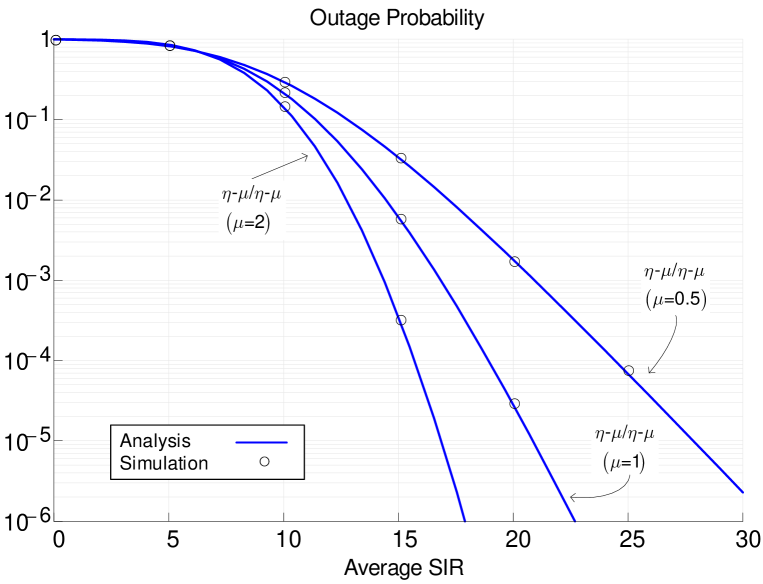
Figure 1: Type I OP expression (7) versus average SIR $\Omega$ for different values of $\mu$, where $\mathcal{S}_{X}\equiv\{\Omega_{X_{n}},\eta_{X_{n}},\mu_{X_{n}}\}_{n=1}^{3}=\{\{\Omega,2.6,\mu\},\{0.8\Omega,3.4,\mu\},\{0.7\Omega,1.7,\mu\}\}$, $\mathcal{S}_{Y}\equiv\{\Omega_{Y_{k}},\eta_{Y_{k}},\mu_{Y_{k}}\}_{k=1}^{3}=\{\{1,3.3,2\},\{1,3.3,2\},\{0.5,1.7,1\}\}$ and $\zeta_{o}=10$.

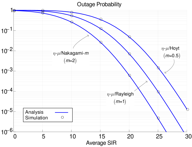
Figure 2: Type II OP expression (8) versus average SIR $\Omega$ for different values of $m$, where $\mathcal{S}_{X}\equiv\{\Omega_{X_{n}},\eta_{X_{n}},\mu_{X_{n}}\}_{n=1}^{2}=\{\{2\Omega,1,0.5\},\{0.7\Omega,0.6,2\}\}$, $\mathcal{G}_{Y}\equiv\{\Omega_{Y_{k}},m_{Y_{k}}\}_{k=1}^{4}=\{\{1,m\},\{1,m\},\{0.5,m\},\{0.2,m\}\}$ and $\zeta_{o}=10$.

Fig. 1 shows some numerical results obtained by the type I OP expression given in (7) for $\zeta_{o}=10$. In this first example, the SOI is formed from three $\eta$-$\mu$ power envelopes ($N=3$) with set of parameters $\mathcal{S}_{X}\equiv\{\Omega_{X_{n}},\eta_{X_{n}},\mu_{X_{n}}\}_{n=1}^{3}=\{\{\Omega,2.6,\mu\},\{0.8\Omega,3.4,\mu\},\{0.7\Omega,1.7,\mu\}\}$; and three $\eta$-$\mu$ interferers ($K=3$) with $\mathcal{S}_{Y}\equiv\{\Omega_{Y_{k}},\eta_{Y_{k}},\mu_{Y_{k}}\}_{k=1}^{3}=\{\{1,3.3,2\},\{1,3.3,2\},\{0.5,1.7,1\}\}$ are considered. Different plots are shown in Fig. 1 in terms of the average signal-to-interference ratio (SIR), which is $\Omega$ in this example, for different values of the parameter $\mu$. Fig. 2 plots the OP for some scenarios included in the type II expression (8) with $\zeta_{o}=10$. In this second example, the SOI is formed from two $\eta$-$\mu$ power envelopes ($N=2$) with set of parameters $\mathcal{S}_{X}\equiv\{\Omega_{X_{n}},\eta_{X_{n}},\mu_{X_{n}}\}_{n=1}^{2}=\{\{2\Omega,1,0.5\},\{0.7\Omega,0.6,2\}\}$; and four Nakagami-$m$ interferers ($K=4$) with $\mathcal{G}_{Y}\equiv\{\Omega_{Y_{k}},m_{Y_{k}}\}_{k=1}^{4}=\{\{1,m\},\{1,m\},\{0.5,m\},\{0.2,m\}\}$ are considered. Again, OP curves are shown in Fig. 1 in terms of the average SIR, which is equal to $\Omega$, for different values of the parameter $m$.

Simulation results are also superimposed in both figures.

V Conclusions

The master formula (1) is derived in this paper, which by appropriate setting of its formal parameters allows us to obtain a variety of elementary closed-form expressions for the outage probability in $\eta$-$\mu$/$\eta$-$\mu$ interference limited scenarios.

Appendix A Proof of Lemma I

Let ${\mathcal{L}}[f(x);x,s]$ or simply ${\mathcal{L}}[f(x);s]$ represent the Laplace transform of $f(x)$ defined as

$${\mathcal{L}}[f\left(x\right);s]\triangleq\int_{0}^{\infty}{e^{-sx}f\left(x\right)dx}.$$ (14)

If $f(x)$ is the probability density function (PDF) of a RV $X$, then its MGF ${\mathcal{M}}_{X}(s)$ is defined as ${\mathcal{M}}_{X}(s)\triangleq{\mathcal{L}}[f\left(x\right);-s]$.

According to [10, eq. 6], the MGF for the sum of independent but arbitrarily distributed $\eta$-$\mu$ RVs $\{X_{n}\}_{n=1}^{N}$, defined in format 1, can be expressed as

$${\mathcal{M}}_{\sum\limits_{n=1}^{N}{X_{n}}}\left(s\right)=\prod\limits_{n=1}^{N}{\left({1-\frac{s}{{\alpha_{2n-1}}}}\right)^{-a_{2n-1}}\left({1-\frac{s}{{\alpha_{2n}}}}\right)^{-a_{2n}}},$$ (15)

where the sets of coefficients $\left\{{a_{\ell}}\right\}_{\ell=1}^{2N}$ and $\left\{{\alpha_{\ell}}\right\}_{\ell=1}^{2N}$ are defined from $\mathcal{S}_{X}$ as specified in (2). Both sets of coefficients are formed by positive real numbers which are not necessarily distinct. The same idea allows us to express the MGF of the sum of the $\eta$-$\mu$ RVs $\{Y_{k}\}_{k=1}^{K}$ as

$${\mathcal{M}}_{\sum\limits_{k=1}^{K}{Y_{k}}}\left(s\right)=\prod\limits_{k=1}^{K}{\left({1-\frac{s}{{\omega_{k}}}}\right)^{-\mu_{Y_{k}}}\left({1-\frac{s}{{\rho_{k}}}}\right)^{-\mu_{Y_{k}}}},$$ (16)

where the set of intermediate coefficients $\mathcal{S}_{Y}^{\star}\equiv\left\{{\omega_{k},\rho_{k}}\right\}_{k=1}^{K}$ is defined according to (3). By hypothesis, the set of parameters $\{{\mu}_{Y_{k}}\}_{k=0}^{K}$ are positive integers; thus, expression (16) can be rearranged as

$${\mathcal{M}}_{\sum\limits_{k=1}^{K}{Y_{k}}}\left(s\right)=\prod\limits_{j=1}^{J}{\left({1-\frac{s}{{\beta_{j}}}}\right)^{-b_{j}}},$$ (17)

where $\left\{{\beta_{j}}\right\}_{j=1}^{J}$ is the set of different values in the set of intermediate coefficients $\mathcal{S}_{Y}^{\star}$, $J$ is the number of different values in $\mathcal{S}_{Y}^{\star}$ and $\left\{b_{j}\right\}_{j=1}^{J}$ is the set of positive integers defined by (4) representing the multiplicities corresponding to $\left\{{\beta_{j}}\right\}_{j=1}^{J}$.

The CDF of $Z={{\sum\limits_{n=1}^{N}{X_{n}}}}/{{\sum\limits_{k=1}^{K}{Y_{k}}}}$ can be expressed through the MGFs of $\sum\limits_{n=1}^{N}{Y_{n}}$ and $\sum\limits_{k=1}^{K}{Y_{k}}$ by appealing to the well-known convolution and scaling properties of the Laplace transform, i.e.

$$\begin{gathered}F_{Z}\left(z\right)=\Pr\left[{\sum\limits_{n=1}^{N}{X_{n}}\leqslant z\sum\limits_{k=1}^{K}{Y_{k}}}\right]=\hfill\\ \quad\quad\int_{0}^{\infty}{F_{\sum\limits_{n=1}^{N}{X_{n}}}\left({zy}\right)f_{\sum\limits_{k=1}^{K}{Y_{k}}}\left(y\right)dy}=\left.{\mathcal{L}\left[{F_{\sum\limits_{n=1}^{N}{X_{n}}}\left({zy}\right)f_{\sum\limits_{k=1}^{K}{Y_{k}}}\left(y\right);y,s}\right]}\right|_{s=0}=\hfill\\ \quad\quad\frac{1}{{2\pi i}}\int\limits_{c-i\infty}^{c+i\infty}{\mathcal{L}\left[{F_{\sum\limits_{n=1}^{N}{X_{n}}}\left({zy}\right);p}\right]}\mathcal{L}\left[{f_{\sum\limits_{k=1}^{K}{Y_{k}}}\left(x\right);-p}\right]dp=\hfill\\ \quad\quad\frac{1}{{2\pi i}}\int\limits_{c-i\infty}^{c+i\infty}{\frac{1}{z}\mathcal{L}\left[{F_{\sum\limits_{n=1}^{N}{X_{n}}}\left(y\right);y,\frac{p}{z}}\right]}\mathcal{L}\left[{f_{\sum\limits_{k=1}^{K}{Y_{k}}}\left(y\right);y,-p}\right]dz=\hfill\\ \quad\quad\frac{1}{{2\pi i}}\int\limits_{c-i\infty}^{c+i\infty}{\Xi\left(p\right)}dp,\hfill\\ \end{gathered}$$ (18)

where the integration kernel

$$\Xi\left(p\right)\triangleq\frac{1}{p}\mathcal{M}_{\sum\limits_{n=1}^{N}{X_{n}}}\left({-\frac{p}{z}}\right)\mathcal{M}_{\sum\limits_{k=1}^{K}{Y_{k}}}\left(p\right),$$ (19)

$i$ is the imaginary unit and $c$ an appropriate real number which splits the singularities of the involved MGFs. Considering (15) and (17), the integration kernel in our case is expressed as

$$\Xi\left(p\right)=\frac{1}{p}\prod\limits_{\ell=1}^{2N}{\left({1+\frac{p}{{z\alpha_{\ell}}}}\right)}^{-a_{\ell}}\prod\limits_{j=1}^{J}{\left({1-\frac{p}{{\beta_{j}}}}\right)}^{-b_{j}}.$$ (20)

Let $\left\{{\hat{\alpha}_{\ell}}\right\}_{\ell=1}^{2N}$ and $\left\{{\hat{\beta}_{j}}\right\}_{j=1}^{J}$ denote the complex-modulus ordered sets corresponding to $\left\{{\alpha_{\ell}}\right\}_{\ell=1}^{2N}$ and $\left\{{{\beta}_{j}}\right\}_{j=1}^{J}$ respectively, i.e. $0\leqslant\left|{\hat{\alpha}_{1}}\right|\leqslant\left|{\hat{\alpha}_{2}}\right|\leqslant\ldots\leqslant\left|{\hat{\alpha}_{2N}}\right|$ and $0<\left|{\hat{\beta}_{1}}\right|<\left|{\hat{\beta}_{2}}\right|<\ldots<\left|{\hat{\beta}_{J}}\right|$; then, the singularity structure of the integration kernel $\Xi(p)$ and the integration paths involved in the computation of the CDF of $Z$ are shown in Fig. 3. Since $\left|{\left.{\Xi\left(p\right)}\right|_{\wp_{\infty}}}\right|\leqslant\frac{C}{R}\prod\limits_{\ell=1}^{2N}{\left({\frac{R}{{z\alpha_{\ell}}}}\right)}^{-a_{\ell}}\prod\limits_{j=1}^{J}{\left({\frac{R}{{\beta_{j}}}}\right)}^{-b_{j}}$ for a sufficiently large $R$ and an appropriate constant $C$, then

$$\mathop{\lim}\limits_{R\to\infty}\left|{\int_{\wp_{\infty}}{\Xi\left(p\right)dp}}\right|\leqslant\mathop{\lim}\limits_{R\to\infty}2\pi R\left|{\left.{\Xi\left(p\right)}\right|_{\wp_{\infty}}}\right|=0.$$ (21)

Thus, the Cauchy-Goursat and the Residue Theorems allows us to express the CDF of $Z$ as follows

$$\begin{gathered}F_{Z}(z)=\frac{1}{{2\pi i}}\int\limits_{\varepsilon-i\infty}^{\varepsilon+i\infty}{\Xi\left(p\right)}dp=\frac{1}{{2\pi i}}\sum\limits_{j=1}^{J}{\int_{\mathcal{C}\left({\beta_{j}}\right)}{\Xi\left(p\right)dp}}-\frac{1}{{2\pi i}}\mathop{\lim}\limits_{R\to\infty}\int_{\wp_{\infty}}{\Xi\left(p\right)dp}=-\sum\limits_{r=1}^{J}{\text{Res}\left[{\Xi;\beta_{r}}\right]}\hfill\\ \quad=-\left({\prod\limits_{j=1}^{J}{\left({-\beta_{j}}\right)^{b_{j}}}}\right)\left({\prod\limits_{\ell=1}^{2N}{\left({z\alpha_{\ell}}\right)^{a_{\ell}}}}\right)\sum\limits_{r=1}^{J}{\frac{1}{{(b_{r}-1)!}}\left.{\frac{{d^{b_{r}-1}}}{{dp^{b_{r}-1}}}}\right|_{\beta_{r}}\left({\frac{1}{p}\prod\limits_{\ell=1}^{2N}{\left({p+z\alpha_{\ell}}\right)^{-a_{\ell}}}\prod\limits_{\begin{subarray}{l}j=1\\ j\neq r\end{subarray}}^{J}{\left({p_{r}-\beta_{j}}\right)^{-b_{j}}}}\right)},\hfill\\ \end{gathered}$$ (22)

where $0<\varepsilon<\left|{\hat{\beta}_{1}}\right|$ and ${\text{Res}\left[{\Xi;\beta_{r}}\right]}$ represents the residue of $\Xi(p)$ at the pole $p=\beta_{r}$. Finally, taking into account the Leibniz derivative rule for products and that

$$\frac{1}{{q!}}\frac{{d^{q}}}{{dx^{q}}}\left({x+a}\right)^{-m}=\frac{{(-1)^{q}\left(m\right)_{q}}}{{\left(1\right)_{q}\left({x+a}\right)^{m+q}}},$$ (23)

the desired expression (1) is obtained after simple algebraic manipulations.

Appendix B Proof of Corollary I

It is clear from (3) that ${\omega_{k}\rightarrow\infty}$ and ${\rho_{k}\rightarrow\frac{{m_{Y_{k}}}}{{\Omega_{Y_{k}}}}}$ when $\eta_{Y_{k}}\rightarrow 0$ and $\mu_{Y_{k}}=m_{Y_{k}}$ for $k=1,\ldots,K$; thus, in this case

$$\mathcal{M}_{\sum\limits_{j=1}^{K}{Y_{k}}}\left(s\right)=\prod\limits_{k=1}^{K}{\left({1-\frac{s}{{\rho_{k}}}}\right)^{-m_{Y_{k}}}},$$ (24)

and the same formal proof given in Lemma I can be repeated from expression (17) by replacing ${\mathcal{S}_{Y}^{\star}}$ with ${\mathcal{G}_{Y}^{\star}}$.

TABLE I: Summary of Some Results Derived in Section III.

Scenario	Assumptions on the Statistical Parameters	OP Expression
$\eta$-$\mu$/$\eta$-$\mu$ Independent MRC	• The $\mu$ parameters of the CCI signals are positive integers.	(7)
Nakagami-$m$/$\eta$-$\mu$ Independent MRC	• The $\mu$ parameters of the CCI signals are positive integers.	(7)
$\eta$-$\mu$/Nakagami-$m$ Independent MRC	• The $m$ parameters of the CCI signals are positive integers.	(8)
Nakagami-$m$/ /Nakagami-$m$ Independent MRC	• The $m$ parameters of the CCI signals are positive integers.	(8)
$\eta$-$\mu$/Rayleigh Independent MRC	• None.	(8)
$\eta$-$\mu$/$\eta$-$\mu$ Correlated MRC	• The $\mu$ parameters of the pre-combining SOI signals are positive integers or half-integers. • The $\mu$ parameters of the CCI signals are positive integers.	(12)
Nakagami-$m$/ /Nakagami-$m$ Correlated MRC	• The $m$ parameters of the pre-combining SOI signals are positive integers or half-integers. • The $m$ parameters of the CCI signals are positive integers.	(13)
$\eta$-$\mu$/Rayleigh Correlated MRC	• The $\mu$ parameters of the pre-combining SOI signals are positive integers or half-integers.	(13)

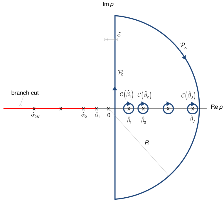
Figure 3: Singularity structure of the integration kernel $\Xi(p)$ and integration paths involved in the proof of Lemma 1.

References

- [1] M. D. Yacoub,’The - and the - distribution,’ IEEE Antennas and Propagation Magazine, vol. 49, pp. 68-81, Feb. 2007.
- [2] D. Morales-Jiménez and J. F. Paris, ’Outage probability analysis for - fading channels,’ IEEE Communications Letters, pp. 521-523, June 2010.
- [3] M. K. Simon and M-S Alouini, Digital Communications over Fading Channels, 2nd ed., John Wiley, 2005.
- [4] K. W. Sowerby and A. G. Williamson, ’Outage probabilities calculations for multiple co-channel interferers in cellular mobile systems,’ IEE Proc. (Pt. F), vol. 135 ,pp. 208–215, June 1988.
- [5] Y. D. Yao and A. U. H. Sheikh, ’Investigation into co-channel interference in microcellular mobile radio systems,’ IEEE Trans. Veh. Technol., vol. 41 ,pp. 114–123, May 1992.
- [6] A. A. Abu-Dayya and N. C. Bealieau, ’Outage probabilities of cellular mobile radio systems with multiple Nakagami interferers,’ IEEE Trans. Veh. Technol., vol. 40 ,pp. 757–768, Nov 1991.
- [7] C. Tellambura and V. K. Bhargava, ’Outage probability analysis for cellular mobile radio systems subject to Nakagami fading and shadowing,’ Trans. IECE Japan, vol. 78-B ,pp. 1416–1423, Oct 1995.
- [8] J. M. Romero-Jerez, J. P. Peña-Martín and A. J. Goldsmith, ’Outage probability of MRC with arbitrary power cochannel interferers in Nakagami fading,’ IEEE Trans. Commun., vol. 55 ,pp. 1283–1286, July 2007.
- [9] V. Asghari, D. B. da Costa and S. Aissa, ’Symbol error probability of rectangular QAM in MRC systems with correlated - fading channels,’ IEEE Trans. Veh. Technol., vol. 59 ,pp. 1497 – 1503, March 2010.
- [10] N. Y. Ermolova, ’Moment generating functions of the generalized - and - distributions and their applications to performance evaluations of communications systems,’ IEEE Communications Letters, pp. 502-504, July 2008.