Simulating structural transitions by direct transition current sampling: the example of LJ₃₈

Abstract

Reaction paths and probabilities are inferred, in a usual Monte Carlo or Molecular Dynamic simulation, directly from the evolution of the positions of the particles. The process becomes time-consuming in many interesting cases in which the transition probabilities are small. A radically different approach consists of setting up a computation scheme where the object whose time evolution is simulated is the transition current itself. The relevant timescale for such a computation is the one needed for the transition probability rate to reach a stationary level, and this is usually substantially shorter than the passage time of an individual system. As an example, we show, in the context of the ‘benchmark’ case of 38 particles interacting via the Lennard-Jones potential (‘LJ₃₈’ cluster), how this method may be used to explore the reactions that take place between different phases, recovering efficiently known results and uncovering new ones with small computational effort.

I Introduction

The evolution of multi-particle systems arising in very diverse domains ranging from biology to material science is often governed by activated processes that occur with very low probability, but have a dramatic effect on the structure. Examples of physical phenomena controlled by such rare events are protein folding in biology, defect diffusion and crystal nucleation in condensed matter physics and cluster rearrangement in chemistry.

Activated events are characterized by the fact that when they occur, their duration is rather short, e.g. of the order of the picoseconds in dense molecular systems, but that, in contrast, the typical time needed for them to start is very large. This separation of time-scale is the very definition of metastability; its origin may be energetic (high barriers) or, more likely in high dimensional systems, at least partly entropic (pathways hard to find). Even though physical times of activated events can be achieved in computer simulation using molecular dynamics, monitoring rare fluctuations is computationally expensive and still remains a challenge because of the long waiting time for the event to occur. To overcome this problem, several different strategies have been developed over the past years. A common idea behind these techniques is to bias the dynamics of the system in order to enhance the occurrence of reaction, or to use previous knowledge of the outcome of the reaction and to fix the endpoint of the trajectory. In order to implement this, in many cases one needs to know an order parameter able to discriminate between the reactant basin, the saddle regions and the product basin.

A set of methods involving the direct sampling of path ensembles has been developed during the last decade. W2003 The strategy is to restrict paths to the subset of reactive paths, those that interpolate between reactant and product basins. Examples of such methods are transition path sampling, DBCD1998 ; BCDG2002 transition interface sampling. VEB2005 Another family of methods such as metadynamics Laio and forward flux sampling VAMFW2007 simulate the evolution in time of the system, and include some form of bias that guarantees that the reaction happens, but then of course the effect of the bias has to be discounted in order to retrieve the true statistics. Methods differ also in the way rate constants are estimated, AVW2009 and the ability to handle nonequilibrium steady states.

Observation of rare events and exploration of energy landscapes of a multi-particle system are indeed two interconnected problems. The requirement of knowing the target of the reaction, and in particular a relevant order parameter that parametrizes the path is problematic in physical situations where nothing a priori is known. Thus, a preliminary step prior to the calculation of finite-temperature rate constants using the sampling techniques mentioned above may consist in locating the saddle points of the energy and the corresponding energy minima using one of the eigenvector following methods described in the literature (e.g. the activation-relaxation technique, MB1998 Optim MW1999 or the dimer method HJ1999 ). The technique in all these methods relies on monitoring the eigenvalues of the Hessian matrix (the matrix of the second derivatives of the potential energy), in order to individuate stable or unstable directions, i.e. minima or saddles. A limitation of these methods is that energy saddles only correspond directly to the actual barriers for the dynamics if the temperature is very low, otherwise the entropic contribution to the dynamics becomes relevant.

Another approach that may be used to explore the free-energy (i.e. finite-temperature) barriers between basins TK2004 ; TTK2006 is inspired by Supersymmetric Quantum Mechanics, which has been used in the context of field theory to derive and generalize Morse Theory, precisely the analysis of the saddle points of a function. Transposing to statistical physics this formalism, one obtains a family of generalizations of Langevin dynamics, converging to barriers and reaction paths of different kinds, rather than to the equilibrium basins. The resulting method involves the evolution in phase space of a population of independent trajectories that are replicated or eliminated according to the value of their Lyapunov exponent.TK2004 The theory guarantees that by selecting trajectories having larger Lyapunov exponents in a specified way, the bias is just what is needed so that the population describes the evolution of the transition current, rather than that of the configurations,TK2006 as they would in an unbiased case. The advantage is that the convergence of the current distribution is much faster than the typical passage time.

In this paper we shall present a more direct and elementary derivation of this dynamics without resorting to quantum theory (section II). Extending the more concise demonstration of Ref. TK2003b, , we will show how the modified dynamics precisely reproduces the evolution in the phase space of the probability current (or more precisely, the ‘transition’ probability current) between equilibrium basins, thus achieving a probability current sampling of the system dynamics. As the transition current evolves in time, it explores the different barriers, indicating which states are reached after different passage times. Starting from an initial equilibrium configuration, far from equilibrium phenomena are easily sampled, as the simulated current is an intrinsically out of equilibrium quantity.TK2004 In section  III, we discuss the actual population dynamic algorithm that may be used to simulate the probability current. Finally, in order to assess the performances of this probability current sampling, we present in section IV an application to the structural transitions of a Lennard-Jones cluster, sampled under different physical conditions. We shall recover known results, and discuss some new ones, obtained in all cases at rather small computational costs.

II Transition currents

II.1 Overdamped Langevin dynamics

Let us consider a 3D many-body system composed of N particles in contact with a thermal bath. We denote $r_{1},\dots,r_{3N}$ the configurational degrees of freedom and $V(\{r_{i}\}_{i=1\dots 3N})$ the interaction potential. In the limit of large friction $\gamma\to\infty$, where inertia can be neglected, the system evolves with a standard overdamped Langevin dynamics

$$\gamma\dot{r_{i}}=-\frac{1}{m_{i}}\frac{\partial V}{\partial r_{i}}+\sqrt{\frac{2\gamma k_{B}T}{m_{i}}}\eta_{i}\;,$$ (1)

where $\eta_{i}$ are independent Gaussian white noises of unit variance and $m_{i}$ correspond to the particle masses.

The probability to find the system at position ${\bf r}\equiv(r_{1},\cdots r_{3N})$ then evolves with the Fokker-Planck equation R1989

$$\frac{\partial P}{\partial t}=\sum_{i}\frac{1}{m_{i}\gamma}\frac{\partial}{\partial r_{i}}\left(k_{B}T\frac{\partial}{\partial r_{i}}+\frac{\partial V}{\partial r_{i}}\right)P\equiv-H_{FP}P\;,$$ (2)

where we have introduced the Fokker-Planck operator $H_{FP}$. We can use the probability current $J_{i}\equiv-\frac{1}{\gamma m_{i}}\left({k_{B}T}\frac{\partial}{\partial r_{i}}+\frac{\partial V}{\partial r_{i}}\right)P$ to write Eq. 2 as a continuity equation for the probability density:

$$\frac{\partial P}{\partial t}+\sum_{i}\frac{\partial J_{i}}{\partial r_{i}}=0\;.$$ (3)

For systems with separation of time scales, the dynamics can be split into two regimes. Starting from an arbitrary probability distribution, $P({\bf r};t)$ relaxes rapidly into a sum of contributions centered on the metastable states. At much longer times, the rare transitions between the metastable states make $P({\bf r};t)$ relax to the equilibrium distribution. Two time scales can also be identified for the dynamics of the probability current. While the probability density rapidly relaxes into the metastable states, the probability current converges on the same time scale to the most probable transition paths between the metastable states. Then, the late time relaxation towards equilibrium corresponds to a progressive vanishing of the current, when forward and backward flux between each metastable state balance. TK2004 Note that the same line of reasoning holds for non-equilibrium systems in which the forces do not derive from a global potential. In such systems, the probability current never vanishes and converges instead to its steady-state value.

If one were able to simulate the evolution of the probability current, one would thus have all the knowledge relevant for the transitions between metastable states, while only having to simulate the system for relatively short time-scales (similar to the equilibration time within a metastable state). As mentioned in the introduction, simulating directly the transition current is the goal of this paper and we now derive a self-consistent evolution equation for $J_{i}$.

Let us define the current operator $\hat{J}_{i}$:

$$\hat{J}_{i}\equiv\frac{1}{\gamma m_{i}}\left(k_{B}T\frac{\partial}{\partial r_{i}}+\frac{\partial V}{\partial r_{i}}\right)\;,$$ (4)

so that the probability current and the Fokker-Planck operator becomes

$$J_{i} =\hat{J}_{i}P$$ (5a)

$$H_{FP} =-\sum_{j}\frac{\partial}{\partial r_{j}}\hat{J}_{j}\;.$$ (5b)

The evolution of the probability current is then given by

$$\dot{J}_{i}=\hat{J}_{i}\dot{P}=-\hat{J}_{i}H_{FP}P=-\sum_{j}\hat{J}_{i}\frac{\partial}{\partial r_{j}}\hat{J}_{j}P\;.$$ (6)

where we have assumed that $H_{FP}$ does not depend explicitly on time. Straightforward algebra shows that $\hat{J}_{i}\frac{\partial}{\partial r_{j}}=\frac{\partial}{\partial r_{j}}\hat{J}_{i}-\frac{\partial^{2}V}{\partial r_{i}\partial r_{j}}$ and $\hat{J}_{i}\hat{J}_{j}=\hat{J}_{j}\hat{J}_{i}$ which turns equation (6) into

$$\dot{J}_{i}=-\sum_{j}\left(\frac{\partial}{\partial r_{j}}\hat{J}_{j}\hat{J}_{i}-\frac{\partial^{2}V}{\partial r_{i}\partial r_{j}}\hat{J}_{j}\right)P\;.$$ (7)

Using the expressions (5a) and (5b) for the currents and Fokker-Planck operator we obtain

$$\dot{J}_{i}=-H_{FP}J_{i}-\sum_{j}\frac{\partial^{2}V}{\partial r_{i}\partial r_{j}}J_{j}\;.$$ (8)

Note that the equations (5a) and (7) are not self-contained: the knowledge of $P({\bf r})$ is required to compute $J_{i}$. On the contrary, (8) depends exclusively on the current, and can readily be used to simulate $J_{i}$, without having to compute $P({\bf r})$ beforehand. The only condition is that the current distribution at the initial time $J_{i}^{0}$ indeed derives from a probability distribution, i.e. is of the form:

$$J_{i}^{0}\equiv-\frac{1}{\gamma m_{i}}\left({k_{B}T}\frac{\partial}{\partial r_{i}}+\frac{\partial V}{\partial r_{i}}\right)P^{0}=-\frac{k_{B}T}{\gamma m_{i}}e^{-\frac{1}{k_{B}T}V}\frac{\partial}{\partial r_{i}}\left[e^{\frac{1}{k_{B}T}V}P^{0}\right]$$ (9)

This means that the initial current distribution should be such that the quantity $A_{i}$

$$A_{i}=m_{i}e^{\frac{1}{k_{B}T}V}J_{i}^{0}$$ (10)

is a gradient, $\frac{\partial A_{i}}{\partial r_{j}}=\frac{\partial A_{j}}{\partial r_{i}}$. A particularly simple initial condition is obtained if one assumes that $P^{0}$ is Gibbsean $P^{0}\propto e^{-\frac{1}{k_{B}T}V}$ in a region $\Omega$, and zero elsewhere. Then, from Eq. (9), $J^{0}_{i}$ is zero everywhere except on the surface of $\Omega$, where it takes the form of a vector normal to the surface of $\Omega$, and with amplitude proportional to the Gibbs weight.

The evolution of current distribution given by Equation (8), starting from an appropriate initial current $J^{0}$ converges to the stationary distribution of currents between metastable states on the same time scale as the usual Langevin equation converges to metastable-state. It is thus not necessary to wait for rare events to identify the transition path between the metastable states, an important improvement over standard MD methods. If there are several metastable states and transitions with different rates, the current distribution at longer times concentrates on the paths between regions that have not yet mutually equilibrated, and vanishes in transitions between states that have had the time to mutually equilibrate.

II.2 Langevin dynamics with inertia

In many physical situations inertia plays an important role and one cannot rely on overdamped Langevin equations. HTB1990 In such case, the stochastic dynamics of $N$ interacting particles is given by

$$\dot{r_{i}} =v_{i}$$ (11a)

$$\dot{v_{i}} =-m_{i}^{-1}\frac{\partial V}{\partial r_{i}}-\gamma\,v_{i}+\sqrt{2m_{i}^{-1}\gamma k_{B}T}\,\eta_{i}\;,$$ (11b)

where $(v_{1},\cdots,v_{n})\equiv{\bf v}$ correspond to the $3N$ velocities.

In order to transpose the derivation of the current evolution given in subsection II.1 to the inertial case, we have to consider the Kramers evolution equation $\dot{P}({\bf r},{\bf v};t)=-H_{K}P({\bf r},{\bf v};t)$ instead of the Fokker-Planck equation: TTK2006

$$\frac{\partial P}{\partial t}=\sum_{i}\left[\frac{\partial}{\partial v_{i}}\left(\frac{\gamma k_{B}T}{m_{i}}\frac{\partial}{\partial v_{i}}+\gamma v_{i}+\frac{1}{m_{i}}\frac{\partial V}{\partial r_{i}}\right)-\frac{\partial}{\partial r_{i}}v_{i}\right]P\;.$$ (12)

As in the overdamped case, this can be written as a conservation equation where the probability current in phase space is given by

$$J_{r_{i}} =v_{i}\,P({\bf r},{\bf v};t)$$ (13a)

$$J_{v_{i}} =-\left(\frac{\gamma k_{B}T}{m_{i}}\frac{\partial}{\partial v_{i}}+\gamma v_{i}+\frac{1}{m_{i}}\frac{\partial V}{\partial r_{i}}\right)P({\bf r},{\bf v};t)\;.$$ (13b)

Once again, the current contains all the information about transitions between metastable states. There is however a conceptual difference: the presence of inertia makes it inherently difficult (and indeed, useless), to compute (13) as it stands. The reason is that the phase-space current

$$J_{r_{i}}=v_{i}P_{\rm eq}\;\qquad J_{v_{i}}=-\frac{1}{m}\frac{\partial V}{\partial r_{i}}P_{\rm eq}\;.$$ (14)

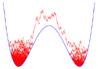
is non-zero even in canonical equilibrium. For example, in a harmonic oscillator $H=\frac{1}{2}\left[v^{2}+r^{2}\right]$ , the phase-space current in equilibrium turns clockwise in circles around the origin.

For this reason, the part of the current that corresponds to transitions between metastable states is screened by the large contributions of the currents within metastable states (see figure 1). The probability current (13a) and (13b) does not really represent the transition paths between metastable states.

We can however define a transition current TTK2006

$$J^{\rm t}_{r_{i}} =J_{r_{i}}+\frac{k_{B}T}{m_{i}}\frac{\partial P}{\partial v_{i}}$$ (15a)

$$J^{\rm t}_{v_{i}} =J_{v_{i}}-\frac{k_{B}T}{m_{i}}\frac{\partial P}{\partial r_{i}}\;,$$ (15b)

which has two interesting properties. Firstly, this current differs from the probability current by a divergenceless term and thus also satisfies the continuity equation $\dot{P}+\nabla\cdot{\bf J^{\rm t}}=0$. Fluxes out of a closed surface surrounding a metastable state are then the same for the probability and transition currents. The latter current thus contains the relevant information about, for instance, transition rates. Secondly, the transition current vanishes in equilibrium, as can be checked by comparing (14) and (15). This current thus contains only the information relevant for the transitions between metastable states (see figure  1) and is not screened by the large ‘equilibrium’ currents within them.

Figure 1: Probability currents for an underdamped dynamics in a 1D double-well potential. Left: Typical transition between the two wells. Center: Same trajectory in phase space. The probability current is dominated by oscillations in the wells. Right: Transition current ${\bf J^{\rm t}}$ in phase space. The transition path is sampled uniformly. Equilibrium contributions are not present.

Using algebra similar to that of the overdamped case, one can show TTK2006 (see the Appendix VI) that the reduced current evolves with

$$\frac{\partial\mathbf{J^{t}}}{\partial t}=-H_{K}\mathbf{J}^{\rm t}-{\mathbf{M}}\cdot\mathbf{J}^{\rm t}\;\;\;\;\;\;with\;\;\;\;\;\;{\mathbf{J^{t}}}=\left(\begin{array}[]{c}J_{r_{i}}^{t}\\ J_{v_{i}}^{t}\end{array}\right)$$ (16)

where the ${6N}\times{6N}$ matrix ${\mathbf{M}}$ is given by

$${\mathbf{M}}=\left(\begin{array}[]{cc}0&-\delta_{ij}\\ \frac{1}{m_{i}}\frac{\partial^{2}V}{\partial r_{i}\partial r_{j}}&\gamma\delta_{ij}\end{array}\right).$$ (17)

Again, (16) is a self-consistent equation for the transition current and we shall now show how it can be simulated.

III Using population dynamics to sample the transition currents

The probability density $P({\bf r},{\bf v})$ is a scalar field that can be obtained by simulating many copies of the system, evolving their positions and velocities with the Langevin equation (11), and constructing histograms. On the contrary, ${\bf J^{\rm t}}$ is a vector field and thus cannot be obtained in the same way: it also requires vectorial degrees of freedom. We first present a population dynamics that can be used to construct the evolution of the transition current in section III.1 and then give the corresponding Diffusion Monte Carlo algorithm in section III.2.

III.1 Stochastic dynamics

For systems with many degrees of freedom, the direct resolution of the partial differential equation (16) yielding the evolution of ${\bf J^{\rm t}}$ is not achievable numerically. In the same way as the Langevin dynamics (11) represents an alternative to the resolution of the Kramers equation, we can use a stochastic dynamics that generates the current evolution (16) numerically.

The explicit construction of the dynamics was already presented in detail in a previous paper. TTK2006 The idea is to proceed in two steps. Firstly, a Langevin dynamics (11) is coupled to a carefully chosen evolution (see below) of a $6N$-dimensional vector ${\bf u}\equiv(u_{r_{1}},\dots,u_{r_{3N}},u_{v_{1}},\cdots,u_{v_{3N}})$ in order to account for the vectorial degrees of freedom of ${\bf J^{t}}$. Secondly, the transition current ${\bf J^{\rm t}}$ is given by the following average:

$${\bf J^{\rm t}}=\int\prod_{i=1}^{6N}\;{\rm d}u_{i}\;{\bf u}\;F({\bf r},{\bf v},{\bf u}).$$ (18)

where $F({\bf r},{\bf v},{\bf u})$ is a joint distribution obtained from the Langevin dynamics, for instance by simulating a large number of copies of the system. foot1

In practice, the coupling between the vectorial and phase space degrees of freedom is obtained by the following population dynamics. One consider ${\cal{N}}$ copies of the system (called ‘clones’), identified by positions and velocities ${\bf r}$ and ${\bf v}$, which all carry a $6N$ dimensional unitary vector ${\bf u}$. The dynamics of each clone is then as follows: TTK2006

• ${\bf r}$ and ${\bf v}$ evolve with the standard Langevin dynamics with inertia (11)

• the vector ${\bf u}$ evolves with

  $$\dot{\bf u}=-{\bf M}\cdot{\bf u}+{\bf u}({\bf u}^{\dagger}{\bf M}{\bf u})$$ (19)

• each clone has a birth-death rate $\alpha=-{\bf u}^{\dagger}{\bf M}{\bf u}$. This is the only way the vector ${\bf u}$ influences the dynamics.

The distribution of clones $F({\bf r},{\bf v},{\bf u})$ then evolves with G1985

$$\frac{\partial F}{\partial t}=-H_{K}F-\sum_{i=1}^{6N}\frac{\partial}{\partial u_{i}}\left[-\sum_{j}M_{ij}u_{j}+u_{i}({\bf u}^{\dagger}{\bf M}{\bf u})\right]F-{\bf u}^{\dagger}{\bf M}{\bf u}F$$ (20)

The first term of the r.h.s. comes from the Langevin dynamics (11), the second one from the evolution of the vector (19) and the last one from the birth-death events. The transition current is then given by (18). On can indeed check that taking the time derivative of the r.h.s of (18) and using (20), one recovers the evolution of the transition current (16) (see previous papers TK2004 ; TTK2006 for more details).

III.2 Algorithm

We first present the implementation of the population dynamics of the clones and then discuss the construction of the transition current. The $m$-th clone is denoted by its phase-space coordinates and vectors at time $t$, $\mathbf{X}_{t}^{m}=\left\{\mathbf{r}^{m}(t),\mathbf{v}^{m}(t),\mathbf{u}^{m}(t)\right\}$. We start with ${\cal{N}}_{c}$ clones whose positions and vectors are arbitrarily chosen. At every time step, the dynamics is as follows:

1. All the vectors ${\bf u}^{m}$ are rescaled to have a unitary norm.

2. The positions and velocities of the clones are propagated using a leap-frog discretized Langevin dynamics. AAC2006 ; AA2008

3. The vectors ${\bf u}^{m}$ evolve with the (leap-frog discretized version of) the following dynamics:

   $$\dot{u}^{m}_{i}=-M_{ij}u^{m}_{j}$$ (21)

   Note that at after this step, the vectors are no more of unitary norm.

4. For each clone one records $w_{m}=||{\bf u}^{m}(t+\delta t)||$.

5. We associate to each clone $m$ a probability weight $\rho_{m}={\cal{N}}_{c}w_{m}/\sum_{i}w_{i}$ and a random number $\epsilon_{m}$ chosen uniformly in $[0,1)$. The clone is then replaced by $y_{m}$ copies, with

   $$y_{m}=\lfloor\rho_{m}+\epsilon_{m}\rfloor$$ (22)

   where $\lfloor x\rfloor$ is the integer part of $x$: if $y_{m}>1$, $y_{m}-1$ new copies of the m-th clone are made. If $y_{m}=0$, the clone is deleted and if $y_{m}=1$, nothing happens. The population size is thus increased by $y_{m}-1$ if $y_{m}>1$ or decreased by $1$ if $y_{m}=0$.

6. After the step 5, the population is rescaled from its current size ${\cal{N}}_{c}^{e}=\sum_{m=1}^{{\cal{N}}_{c}}y_{m}$ to its initial size ${\cal{N}}_{c}$, by uniformly pruning/replicating the clones.

Steps 1 to 3 correspond to the propagation step of independent clones, whereas steps 4 to 6 correspond to selection steps. In particular, the steps 4 and 5 correctly represents the cloning rate $\alpha=-{\bf u^{\dagger}Mu}$ of the previous subsection since $\frac{\rm d}{{\rm d}t}||{\bf u}^{m}(t)||=-{{\bf u}^{m}}^{\dagger}{\bf M}{\bf u}^{m}$, so that $||{\bf u}^{m}(t+\delta t)||\simeq\exp(-\delta t{{\bf u}^{m}}^{\dagger}{\bf M}{\bf u}^{m})$.

The rescaling of the population at the step 6 can be done in many ways. For instance, one can pick a new clone at random ${\cal{N}}_{c}$ times among the ${\cal{N}}_{c}^{e}$ clones obtained at the end of the step 5. We used an alternative approach that is less costly in terms of data manipulations: if ${\cal{N}}_{c}^{e}>{\cal{N}}_{c}$, we kill ${\cal{N}}_{c}^{e}-{\cal{N}}_{c}$ clones chosen uniformly at random among the ${\cal{N}}_{c}^{e}$ obtained at the end of the step 5. Conversely, if ${\cal{N}}_{c}^{e}<{\cal{N}}_{c}$, we choose uniformly at random ${\cal{N}}_{c}-{\cal{N}}_{c}^{e}$ clones and duplicate them. Note that even though the clones evolve independently during the propagation step, their dynamics are correlated because the deleted clones are replaced by the duplicated ones at the selection steps. When the probability weights of the clones are all equal, we have $\rho_{m}=1$ and $y_{m}=1$. As a result, the population is left unchanged. Conversely, when the clone weights take distinct values, clones with small weights are likely to be replaced by those with large weights.

There are many ways of implementing the resampling of the population (steps 5-6), well documented in the literature on Diffusion Monte Carlo. MJL2007 ; C2007 In particular, it could be advantageous to do the resampling only every $n$ time steps, where $n$ is tuned to ensure ergodicity in phase space, i.e. to achieve enhanced sampling towards the unstable regions where saddles are located.

Since the clones move in phase space with a Langevin dynamics, it can be surprising that they converge rapidly to the reaction paths, i.e. that they explore efficiently the transition states. This can however be understood by noting that their dynamics (without taking the averages (18)) is the so-called Lyapunov Weighted Dynamics TK2006 which is used to bias the Langevin dynamics in favor of chaotic trajectories. The clones will then tend to ‘reproduce’ favorably in the neighborhood of saddles, which are particularly chaotic regions of phase space, and to die in wells. This generates an ‘evolutionary pressure’ that helps the clone escape from metastable states and find the reaction paths.

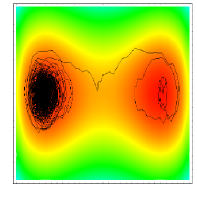
As mentioned before, this dynamics does not provide directly the transition current and one still has to construct the averages (18). This can be difficult and clever methods to do so were discussed in the literature, for instance by Mossa and Clementi who studied the folding of chain of aminoacids. MC2007 The difficulty is connected to the well-known sign problem: large population of clones with arrows pointing in opposite directions cancel in the average but can numerically screen smaller asymmetric distribution that contains the information relevant for the transition current. One can however show that if one starts from a population of clones uniformly spread over a reaction path separating two metastable states and pointing in the same direction, the time taken for the sign problem to occur is of the order of the tunneling time through the barrier (see Appendix VII). In the following we will always simulate much shorter times and omit the averaging steps to simply look at the distribution of clones. This distribution often suffices to locate the reaction paths, as can be seen on figure 1 for the double well potential. To extract further information, for instance regarding the reaction rates, we would need to do the averages, as was done in Ref. MC2007, , but this is beyond the scope of this article.

IV Applications

IV.1 LJ₃₈ cluster

We now turn to the study of transitions between metastable states in the 38-atom Lennard-Jones cluster, a benchmark model system that has been extensively investigated in the past. DMW1999b ; DMW1999 ; NCFD2000 ; CNFD2000 ; AAC2006 This system has a complex potential energy landscape organized around two main basins: a deep and narrow funnel contains the global energy minimum, a face-centered-cubic truncated octahedron configuration (FCC), while a separate, wider, funnel leads to a large number of incomplete Mackay icosahedral structures (ICO) of slightly higher energies.

Although the lowest potential energy minimum corresponds to the FCC structure, the greater configurational entropy associated to the large number of local minima in the icosahedral funnel make this second configuration much more stable at higher temperatures. As temperature increases, this system thus undergoes the finite-size counterpart of several phase transitions. First, a solid-solid transition occurs at $T_{ss}=0.12\frac{\epsilon}{k_{B}}$ when the octahedral FCC structure gives place to the icosahedral ones. At a slightly higher temperature, $T_{sl}=0.18\frac{\epsilon}{k_{B}}$, the outer layer of the cluster melts, while the core remains of icosahedral structure. MF2006 This ‘liquid-like’ structure, also referred to as anti-Mackay in the literature, then completely melts around $T_{sl}=0.35\frac{\epsilon}{k_{B}}$. MF2006

The numerical study of this system is challenging: global optimization algorithms have failed to find its global energy minimum for a long time W2003 and direct Monte Carlo sampling fails to equilibrate the two funnels. The study of the equilibrium thermodynamics of this system required more elaborate algorithms such as parallel tempering, NCFD2000 ; CNFD2000 ; MF2006 basin-sampling techniques, BWC2006 Wang-Landau approaches PCABD2006 or path-sampling methods. AAC2006 ; MP2007 ; AM2010

More recently, the dynamical transitions between the two basins has been studied following various approaches. The interconversion rates between the FCC and ICO structures have been computed using Discrete Path Sampling. W2002 ; W2004 ; BW2006 This elaborate algorithm relies on the localization of minima and saddles of the potential energy landscape, using eigenvector following, and then on graph transformation TW2006 to compute the overall transition rate between two regions of phase space. To the best of our knowledge, this is the most successful approach as far as computing reaction rates in LJ₃₈ is concerned. TW2006 However, the numerical methods involved are quite elaborate, require considerable expertise and have a number of drawbacks, all deriving from the fact that it is based on the harmonic superposition approximation and the theory of thermally activated processes. It thus requires any intermediate minima between the two basins to be equilibrated and this is only possible for small enough systems at low temperatures. W2002 More importantly, when the difficulty in going from one basin to the other is due to entropic problems, as is the case for instance in hourglass shaped billiards, then the knowledge of minima and saddles of the potential energy landscape is not sufficient.

Another attempt to study the transitions between the two funnels of LJ₃₈ relies on the use of transition path sampling. MP2007 Because of the number of metastable states separating the two main basins, the traditional shooting and shifting algorithm failed here, despite previous success for smaller LJ clusters. DBC1998 The authors thus developed a two-ended approach which manages to successfully locate reaction paths between the two basins: they started from a straight trial trajectory linking the two minima, and obtained convergence towards trajectories of energies similar to those obtained in the Discrete Path Sampling approach. MP2007 Although the authors point out the lack of ergodicity in the sampling within their approach and the sensitivity on the ‘discretization’ of the trajectories, this is nevertheless a progress and the main drawback remains the high computational cost (the work needed $10^{5}$ hours of cpu time) to obtain such converged trajectories. In contrast, the simulations we present below required less than $10^{2}$ hours of cpu time.

IV.2 The LJ₃₈ cluster and bond-orientational order parameters

Before presenting our simulations results, we give some technical details on the LJ₃₈ system and on the visualization of the different metastable states. The Lennard-Jones potential is given by the expression

$$V\left(\left\{\mathbf{r}^{j}\right\}_{j=1,...,N}\right)=4\epsilon\sum_{j<k}\left[\left(\frac{\sigma}{r_{jk}}\right)^{12}-\left(\frac{\sigma}{r_{jk}}\right)^{6}\right]$$ (23)

where $\mathbf{r}^{j}=(r^{j}_{x},r^{j}_{y},r^{j}_{z})$ is the position of the $j$-th atom, $r_{jk}=\left|\mathbf{r}^{j}-\mathbf{r}^{k}\right|$ is the distance between atoms $j$ and $k$, $\epsilon$ is the pair well depth and $2^{1/6}\sigma$ is the equilibrium pair separation. In addition, all the particles are confined by a trapping potential that prevents evaporation of the clusters at finite temperature (i.e. particles going to infinity). If the distance between the position ${\bf r}$ of a particle and the center of the trap ${\bf r_{c}}$ exceeds $2.25\sigma$, then the particle feels a potential $|{\bf r}-{\bf r_{c}}|^{3}$. LJ reduced units of length, energy and mass ($\sigma=1,\epsilon=1,m=1$) will be used in the sequel so that the time unit $t=\sigma\sqrt{m/\epsilon}$ is set to $1$.

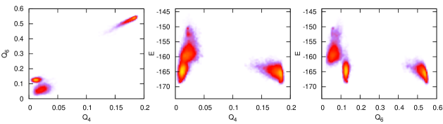
Rather than listing the 228 degrees of freedom of the atomic cluster, configurations are traditionally described using the $Q_{l}$ bond-orientational order parameters SNR1981 ; SNR1983 that allow to differentiate between various crystalline orders

$$Q_{l}=\left(\frac{4\pi}{2l+1}\frac{1}{{{N}}_{b}^{2}}\sum_{m=-l}^{l}\left|Y_{lm}\left(\theta_{jk},\phi_{jk}\right)\right|^{2}\right)^{1/2}\;,$$ (24)

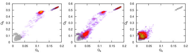
where the $Y_{lm}(\theta,\phi)$ are spherical harmonics and $\theta_{jk},\phi_{jk}$ are the polar and azimuthal angles of a vector pointing from the cluster center of mass to the center of the (j,k) bond which connects one of the $N_{b}$ pairs of atoms. foot2 The parameter $Q_{4}$ is often used to distinguish between the icosahedral and cubic structures, for which it has values around 0.02 and 0.18 respectively. NCFD2000 $Q_{4}$ however does not distinguish between the icosahedral and the liquid-like phase and one thus often uses $Q_{6}$, for which FCC, icosahedral and the liquid-like phase take values around $0.5$, $0.13$ and $0.05$, DMW1999 respectively. To show the spread of the various basins in the $(Q_{4},Q_{6})$ plane, we ran several molecular dynamic simulations, long enough to equilibrate within each basin but short enough so that one does not see tunneling (see figure 2).

Figure 2: Short MD simulations were run to give an impression of the spread in the (Q6,Q4,E) space of each ‘phases’. The simulation time was short enough that no tunneling between the phases was observed. The temperature was set to $T=0.15$. The positions of the phases barely move in the $(Q_{4},Q_{6})$ plane when the temperature changes, although their spreading does. The kinetic energy however shifts when the temperature changes, and is roughly proportional to $NkT$ where $N$ is the number of degrees of freedom.

Although the whole temperature scale is interesting, the challenging part from a computational point of view is the low-temperature regime where ergodicity is difficult to achieve. Below, we show the results of our algorithm for three temperatures: $T=0.12\epsilon/k_{B}$, $T=0.15\epsilon/k_{B}$ and $T=0.19\epsilon/k_{B}$ that span the ranges around the solid-solid and partial melting transitions.

IV.3 Simulations

Given the high dimensionality of the system, it is difficult to follow the evolution of all the coordinates of the clones in order to know if they have localized interesting structures. Instead, we proceed as follows: we plot the evolution of the average over the clone population of $Q_{4}$, $Q_{6}$ and $E$ as a function of the simulation time and we frequently store the positions and velocities of all the clones.

If we see a plateau in $Q_{4}(t)$, $Q_{6}(t)$ and $E(t)$, two cases are possible: either the clones have converged to a reaction path, or they are stuck in a metastable basin. In order to distinguish the two situations, we run an auxiliary short molecular dynamic simulation (without cloning) starting from the positions and velocities of the clones. The duration of this auxiliary simulation is long enough to observe relaxation into the metastable basins, but much shorter than the transition times. If the clones evolve away from the region they had populated in phase-space, we know they had found a reaction path and the auxiliary MD simulation converges to the metastable basins connected by this reaction path. If on the other hand the clones do not evolve away, we know that they had been stuck in some local basin. In such a case we can change two parameters to enhance the sampling of the phase space: the number of clones and the friction $\gamma$ (see below for more details). The time step is always $\delta t=0.01$. Note that this procedure could be automated, but the way to do so is let for future work.

In principle, any observable that can measure whether the population of clones splits in two separate sub-populations after a short Langevin dynamics would be suitable. If the clone population splits in two subpopulations with the same $Q_{4}$, $Q_{6}$ and $E$, we may fail to detect the corresponding barrier. However, this coincidence would be extremely unlikely.

Last, in addition to help us localize barriers, these short Langevin simulations allows us to explore the true dynamics close to a particular transition states.

IV.3.1 $T=0.15$

We first ran several simulations at $T=0.15$, where the most stable state is the MacKay icosahedral minimum (ICOm) while the liquid-like phase (ICOam) and the FCC basin are metastable.

Starting from the ICOm basin with ${\cal{N}}=200$ clones and a low friction $\gamma\delta t=10^{-3}$, the clones rapidly find ($t\sim 1500$) a transition path to the liquid-like phase ICOam. Later on ($t\sim 3500$) an activated event bring the clones to another reaction path that points towards the FCC funnel. These times have to be compared with the transition time between the ICOm and FCC basins that was previously evaluated in the literature at roughly $10^{7}$. W2002 Note that each barrier or path act as a metastable state for the cloned dynamics and it is by activation that the population jumps from one barrier to another. Running the same dynamics with a larger number of clones (${\cal{N}}=600$) tends to stabilize the first barrier so that one has to wait longer to see the transition to the second one.

Starting from the FCC minimum with the same number of clones and at the same friction results in the clones rapidly going out of the FCC funnel and falling in the amorphous zone at the entrance of the icosahedral funnel. NCFD2000 A reaction path is followed by the clones but not maintained. To stabilize this reaction path, we increased the number of clones and the friction. The effect of the former is mostly to slow down the dynamics while the latter allow the clones to populate the reaction path more uniformly. For ${\cal{N}}=600$ clones and $\gamma\delta t=1$, the population of clones indeed stabilizes the reaction path leading from the FCC basins to the entrance of the icosahedral funnel. The reason why we need more clones to stabilize this barrier than the ones in the icosahedral funnel is probably that the former is more flat and spread than the latter ones DMW1999 and thus requires a larger number of clones to be sampled uniformly.

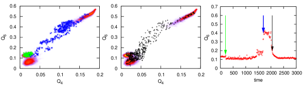
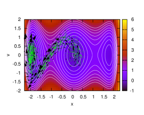
All these results are plotted on figure 3, in which we show the three basins ICOm, FCC and ICOam obtained from the initial MD simulations (see figure 2) and the positions of the clones in the $(Q_{4},Q_{6})$ and $(Q_{6},E)$ plans at different simulation times.

Figure 3: Left and Center: Positions of the clones starting from the ICOm and FCC minima in the $(Q_{4},Q_{6})$ and $(Q_{6},E)$ plans at $T=0.15$. The clones starting from the icosahedral basin first find the barrier between ICOm and ICOam (black symbols, $t=1850$). They then fall back in the ICO basin before finding a path that points towards the FCC funnel (blue symbols, $t=3500$). Starting from FCC, the $600$ clones find a path that leads toward the icosahedral funnel (green symbols, $t=1500$). Right: We plot $Q_{6}$ as a function of time for the clones starting from the ICOm basins (red symbols) and the FCC basin (magenta symbols). Arrows indicates the time at which the snapshots shown in the left and center panel are taken.

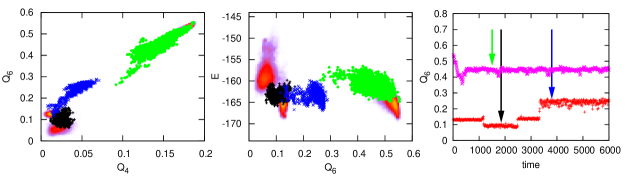
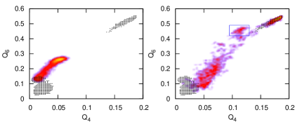
To identify the various metastable basins connected by the clones, we ran several short MD simulations starting from the two long-lived plateaux (blue and green arrows in the right panel of figure 3). Histograms made from these MD runs are shown in figure 4. They show that the clones going out of the ICO basin find barriers toward the amorphous region at the entrance of the ICO funnel while the ones starting from the FCC minimum find a reaction path between the FCC basin and the icosahedral funnel. Interestingly, this path goes through a faulty FCC basin located around $(Q_{4},Q_{6})=(0.12,0.45)$ that has been previously reported in the literature. NCFD2000 ; AAC2006

Figure 4: Histograms made at the end of short MD simulations at $T=0.15$ started from the clones positions at the times indicated by the green and blue arrows in figure 3. The gray-dotted regions correspond to the equilibrium MD simulations of the three basins ICOm, ICOam and FCC. Left: MD simulations started from the stationary structures found by the clones in the ICO funnel fall either back into the ICO basin or in a metastable basin around $(Q_{4},Q_{6})=(0.3,0.05)$ that corresponds to an amorphous structure at the entrance of the ICO funnel. Center: The clones starting from the stable structure found in the FCC funnel fall either back in the FCC basin, or in a faulty FCC metastable state (blue rectangle) or in the ICO funnel, which. Both structures thus correspond to reaction paths. Right: Position of the surface atoms of a clone that has fallen in the faulty FCC configuration after the short MD. This figure was made using a Mathematica Spreadsheet that can be downloaded at %****␣Article_arxiv_up.tex␣Line␣850␣****http://www-wales.ch.cam.ac.uk/~wales/make_frames.nb.

The clones have thus found reaction paths pointing out of their starting funnels. The clones starting from the FCC basins find a reaction path that leads into the icosahedral funnel while the one started from the ICOm basin still remain in the icosahedral funnel. This could be explained by the fact that at this temperature ICOm is the stable state while FCC is only metastable so that the barrier ICO$\to$FCC has to be harder to access than the one from the FCC side. Running short MD starting from the clones positions reveal intermediate metastable basins, either a faulty FCC or amorphous structures.

IV.3.2 $T=0.12$

This is the coexistence temperature between the ICOm and FCC minima. At such a low temperature, more and more secondary barriers play a role so that the transition between ICO and FCC becomes more and more complex. From the point of view of the time evolution of the transition current, this means that there are more and more metastable states for the clone dynamics.

Starting from the ICOm basin with 600 clones and $\gamma\delta t=10^{-3}$, we once again locate the barrier between ICOm and liquid-like phase ICOam. At this temperature this barrier is long-lived and we do not locate the one previously found at $T=0.15$ that points toward the entrance of the icosahedral funnel.

Starting from the FCC basin with $\gamma\delta t=0.02$, the $600$ clones find several barriers that constitute a multi-step reaction path toward the icosahedral funnel. Once again, the larger the friction the longer the clones spend on intermediate barriers.foot3

Figure 5: Left and Center: Positions of the clones starting from the ICOm and FCC minima in the $(Q_{4},Q_{6})$ and $(Q_{6},E)$ plans at $T=0.12$. The clones starting from ICO find the barrier between ICOm and ICOam (black symbols, $t=8000$). Starting from FCC, the clones find a succession of barriers that leads toward the icosahedral funnel (green symbols at $t=650$, blue symbols at $t=1300$ and cyan symbols at $t=2650$). Right: We plot $Q_{6}$ as a function of time for the clones starting from the ICOm basins (red symbols) and the FCC basin (magenta symbols).

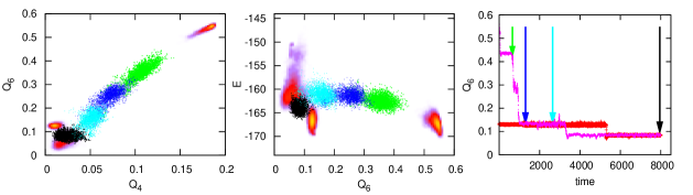
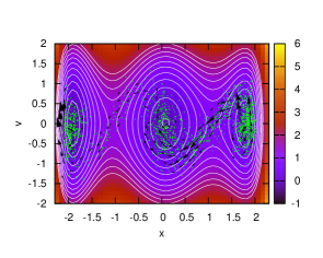
The position of the clones corresponding to the successive metastable barriers are shown in figure 5. Note that the typical times needed for locating the barriers are of the order of $10^{3}$, that is seven orders of magnitude smaller than the reaction times between ICOm and FCC, which is of the order of $10^{10}$. W2002

Figure 6: The color codes correspond to MD simulations at $T=0.12$ started on the green (left), blue (center) and black (right) arrows in figure 5. Left: Starting from the first stationary structure found in the FCC funnel, the clones relaxes mostly in the FCC basin and in the faulty FCC configuration shown in 4. Center The second barrier is close to the commitor between the ICO and the FCC funnel: the clone population relaxes almost equally in both funnel ($57\%$ of the clones fall back in the icosahedral funnel while $43\%$ enter the fcc funnel). Right Clones started from the barrier between ICOm and ICOam populate both basins. Note that the relaxation is much slower than for the other barrier because of the entropic nature of this barrier.

Running short MD simulations starting from the clone positions on the barriers and constructing the corresponding histograms reveals various intermediate metastable basins in the ICO and FCC funnels (See figure 6 ). The fact that $Q_{4}$ and $Q_{6}$ are not good reaction coordinates is confirmed in this figure: the first plateau (green points on figure 5) seems to be after the faulty configuration when going from the FCC funnel to the icosahedral one but the MD starting from this barrier falls into the faulty configuration and the FCC basin, which seems to indicate that this barrier is a reaction state between the FCC and the faulty configuration. There is then a second barrier between the faulty FCC and the ICO funnel (blue dots in figure 5). A last barrier leads to the amorphous region that separates the liquid-like phase and ICOm minimum. Note that in these regions the MD simulations are not very helpful because the transition between ICOm and ICOam has an entropic nature so that it is difficult to relax into the basins. The clones, however, successfully identify the barrier between these two states.

IV.3.3 $T=0.19$

This temperature is very close to the transition between ICO and liquid-like phase. As shown by free-energy studies, the barrier between the FCC and the ICO funnels is very low and the FCC basin is rather unstable. DMW1999 Clones starting from the FCC basin do not stabilize on any structure because there is no proper ‘rare barrier’ and MD simulations starting from FCC immediately falls into the icosahedral funnel. DMW1999

Starting $100$ clones from the ICO basin at $\gamma\delta t=0.01$, they rapidly find a barrier connecting to the liquid-like phase. Later on, activated events lead the clones to locate a reaction path leading towards the FCC funnel. Starting MD from this barrier show that the clones relax into the FCC and ICO funnel.

Figure 7: Left: $100$ Clones are started at $T=0.19$ in the ICOm basin where they spend some time (first first time steps after $t=200$, green dots) before locating the barrier toward the FCC funnel (first five time steps after $t=1700$, blue crosses). Center: When the clones have found the barrier ($t=2000$) a standard MD starts and relaxes as it should into the two funnels (black dots, five first snapshots after $t=2050$). Right: Evolution of $Q_{6}(t)$. The cloning is stopped at $t=2000$ and a normal MD follows.

As mentioned above, it is hard for the clones to stabilize because the FCC funnel is barely metastable and the barrier crossed while going from FCC to ICO is rather flat at this temperature. It is thus quite surprising that they nevertheless manage to do so while starting from the ICO basin. If one starts from the FCC funnel, the clones almost immediately fall into the ICO funnel and then from there can locate the barrier again, but we were not able to stabilize the barrier when coming from the FCC basin. This might be due to the fact that clones stabilize reactions that take place on long time-scale (ICO$\to$FCC), but not short-time relaxations (FCC$\to$ICO).

IV.4 $T=0.05$: annealing the cloned system

Figure 8: Left: Result of a simulation run at T=0.12 with 600 clones, starting from the FCC minimum, with $\gamma\delta t=0.6$ Right: Starting from the end point of the simulations at T=0.12, we run a standard cloning simulation at $T=0.05$. After a time $t=1790$ the 600 clones are still on the structure that had localized at $T=0.12$, which is thus very stable.

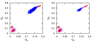
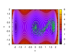
If one starts at such a low temperature from one of the various metastable basins, the clones remain trapped for a time longer than the simulation time. One can however use a temperature annealing to locate the barriers. If one starts the cloning simulation at $T=0.12$ or higher, it is quite easy, as we saw above, to localize the barriers. The temperature can then be decreased to $T=0.05$ and the clones remains on the structure that were localized at a higher temperature (see figure 8).

V Conclusions

The algorithm we have discussed in this paper may be characterized as one that simulates the evolution in time of the current distribution, rather than that of the configuration. Because the time for the escape current to be established is often much smaller than the passage time itself, the method is able to find the transition paths very efficiently.

The method has several attractive features:

i) It does not require any previous knowledge of the relevant reaction coordinates. On the other hand, if an approximation of the reaction path is known a priori, one may always start the clones along this path, and they will populate the true current distribution in a shorter time.

ii) Because the target of the dynamics is the reaction path distribution itself, one may perform simulated annealing in path space: first populating the reaction path corresponding to relatively high temperature, and then refining it to the lower, target temperature. Repeated annealing can also be used to locate several competing barriers in system with multiple reaction mechanisms.

iii) The reaction current vanishes between mutually thermalized regions. foot4 This is why at longer times, the system converges to the barriers that take longer to cross, irrespective of whether they are of entropic or energetic nature. This may be an advantage in cases in which the energy landscape is not in itself dominant, but rather the multiplicity of paths dominates.

iv) The construction of the transition current and the cloning algorithm also applies for non-equilibrium systems where the forces derive locally, but not globally from a potential, such as a system with leads at the edges having a potential difference. Reaction paths between non-equilibrium metastable states, which cannot be described in term of a free energy, may be studied in the same way. The only difference is that the average (18) does not vanish in the long time limit and converges instead to the steady-state transition current.

Note that since the method does not require the knowledge of the reaction coordinate, it could be used efficiently in systems with competing reactions where one does not know a priori the end points of the reaction paths. This would for instance be particularly interesting when studying the crystallization of suspensions of oppositely charged colloids. SVFD2007 ; P2009

In principle, the reaction time may be expressed directly in terms of the (unnormalized) reaction current. It may also be recovered from the weights carried by the clones, which may possibly be achieved from importance sampling in a Lyapunov-weighted ensemble of trajectories. GD2010 However, the method, as it stands does not allow one to calculate the reaction time with great precision, due to the exponential nature of the timescale. Further work is required in this direction.

Acknowledgement: We thank the ESF programme “SimBioMa - Molecular Simulations in Biosystems and Material Science”(M.P.) and EPSRC Ep/H027254 (J.T.) for funding, D. Wales and C. Valeriani for repeated fruitful discussions and F. Calvo and D. Wales for giving us several numerical routines.

VI Appendix A

We report here the derivation of the time evolution equation (16) for the transition current in the underdamped (i.e., Kramers) case of section II.2.

The classical Kramers probability current $\mathbf{J}$, presented in equations (15) , can indeed be written, as in the Fokker-Planck case (Eq. (5a)), in the operatorial form $\mathbf{J}(\mathbf{r},\mathbf{v},t)=\hat{\mathbf{J}}P(\mathbf{r},\mathbf{v},t)$, where the components of the current Kramers operator are

$$\hat{J}_{r_{i}}= {v_{i}}$$ (25a)

$$\hat{J}_{v_{i}}= -\left(\beta^{-1}\frac{\gamma}{m_{i}}\frac{\partial}{\partial v_{i}}+\gamma v_{i}+\frac{1}{m_{i}}\frac{\partial V}{\partial r_{i}}\right)$$ (25b)

In equations (15) of section II.2, a transition current $\mathbf{J}^{t}$ has been introduced, which can be expressed in turn with operators as

$$\mathbf{J}^{t}=\mathbf{\hat{\mathbf{J}}}^{t}P=\left(\hat{\mathbf{J}}+\hat{\mathbf{T}}\right)P$$ (26)

where $\mathbf{\hat{\mathbf{J}}}$ is the Kramers current operator reported above, giving the usual phase-space current $\mathbf{J}$, and the ‘transition’ operator

$$\hat{\mathbf{T}}_{r_{i}} = \frac{1}{\beta m_{i}}\frac{\partial}{\partial v_{i}}$$

$$\hat{\mathbf{T}}_{v_{i}} = -\frac{\partial}{\partial r_{i}}$$ (27)

$\hat{\mathbf{T}}P$ is a divergenceless term. As already remarked in section II.2, the transition current still satisfies the continuity equation

$$\frac{\partial P}{\partial t}=-\nabla_{\mathbf{r},\mathbf{v}}\cdot\mathbf{J}^{t}$$ (28)

thanks to the divergenceless of $\hat{\mathbf{T}}P$. We have introduced here the phase-space divergence $\nabla_{\mathbf{r},\mathbf{v}}\equiv(\nabla_{\mathbf{r}},\nabla_{\mathbf{v}})$

As in section II.1, we proceed now in deriving explicitly the time evolution equation of $\mathbf{J}^{t}$. Multiplying both sides of the continuity equation above (indeed identical to the Kramers equation (12)) by the transition current operator leads to

$$\hat{\mathbf{J^{t}}}\frac{\partial P}{\partial t}=-\hat{\mathbf{J^{t}}}\nabla_{\mathbf{r},\mathbf{v}}\cdot\hat{\mathbf{J^{t}}}P$$ (29)

On the l.h.s. the transition current operator can be commuted with the time derivative. The r.h.s. of (29) can be rewritten with commutators as

$$\hat{\mathbf{J}}^{t}\nabla_{\mathbf{r},\mathbf{v}}\cdot\hat{\mathbf{J}}^{t}=\nabla_{\mathbf{r},\mathbf{v}}\cdot\hat{\mathbf{J}}\left(\hat{\mathbf{J}}+\hat{\mathbf{T}}\right)+\left[\hat{\mathbf{J}},\nabla_{\mathbf{r},\mathbf{v}}\cdot\hat{\mathbf{J}}\right]+\left[\hat{\mathbf{T}},\nabla_{\mathbf{r},\mathbf{v}}\cdot\hat{\mathbf{J}}\right]$$ (30)

using  (29) and the zero divergence property of $\hat{\mathbf{T}}$.

Resorting to definitions of the current operator $\hat{\mathbf{J}}$ and the transition operator $\hat{\mathbf{T}}$ given in  (25a), (25b) and  (VI), explicit expressions for commutators in  (30) can be recovered with straightforward algebra: the term $\left[\hat{\mathbf{J}},\nabla_{\mathbf{r},\mathbf{v}}\cdot\hat{\mathbf{J}}\right]$ gives

$$\left[\hat{J}_{r_{a}},\nabla_{\mathbf{r},\mathbf{v}}\cdot\hat{\mathbf{J}}\right]P =-\sum_{i}\delta_{ia}\left(J_{v_{i}}-\frac{\gamma}{\beta m_{i}}\partial_{v_{i}}\right)P$$ (31a)

$$\left[\hat{J}_{v_{a}},\nabla_{\mathbf{r},\mathbf{v}}\cdot\hat{\mathbf{J}}\right]P =\sum_{i}\delta_{ia}\left(\gamma J_{v_{i}}-\frac{\gamma}{\beta m_{i}}\partial_{r_{i}}\right)P-\sum_{i}\frac{1}{m_{i}}\frac{\partial^{2}V}{\partial r_{i}\partial r_{a}}v_{i}P$$ (31b)

while $\left[\hat{\mathbf{T}},\nabla_{\mathbf{r},\mathbf{v}}\cdot\hat{\mathbf{J}}\right]$ can be expressed as

$$\left[\hat{T}_{r_{a}},\nabla_{\mathbf{r},\mathbf{v}}\cdot\hat{\mathbf{J}}\right]P =\sum_{i}(\beta m_{i})^{-1}\delta_{ia}\left(\partial_{r_{i}}+\gamma\partial_{v_{i}}\right)P$$ (32a)

$$\left[\hat{T}_{v_{a}},\nabla_{\mathbf{r},\mathbf{v}}\cdot\hat{\mathbf{J}}\right]P =\sum_{i}(\beta{m_{i}}^{2})^{-1}\frac{\partial^{2}V}{\partial r_{i}\partial r_{a}}\partial_{v_{i}}P$$ (32b)

Inserting now  (31) and  (32) in the r.h.s. of Eq. (29) yields

$$(\hat{J}_{r_{a}}+\hat{T}_{r_{a}})(\nabla_{\mathbf{r},\mathbf{v}}\cdot\hat{\mathbf{J}})P =(\nabla_{\mathbf{r},\mathbf{v}}\cdot\hat{\mathbf{J}})J_{r_{a}}^{t}-\sum_{i}\delta_{ia}(J_{v_{a}}-\gamma(\beta m_{i})^{-1}\partial_{v_{i}}P)$$

$$\hskip 56.9055pt+\sum_{i}(\beta m_{i})^{-1}\delta_{ia}(\partial_{r_{i}}+\gamma\partial_{v_{i}})P$$ (33a)

$$(\hat{J}_{v_{a}}+\hat{T}_{v_{a}})(\nabla_{\mathbf{r},\mathbf{v}}\cdot\hat{\mathbf{J}})P =(\nabla_{\mathbf{r},\mathbf{v}}\cdot\hat{\mathbf{J}})J_{v_{a}}^{t}+\sum_{i}\delta_{ia}(\gamma J_{v_{a}}-\frac{\gamma}{\beta m_{i}}\partial_{r_{i}}P+\frac{1}{m_{i}}\frac{\partial^{2}V}{\partial r_{i}\partial r_{a}}J_{r_{i}})$$

$$\hskip 56.9055pt+\frac{1}{\beta{m_{i}}^{2}}\frac{\partial^{2}V}{\partial r_{i}\partial r_{a}}\partial_{v_{i}}P$$ (33b)

that can be recasted as

$$\mathbf{\hat{\mathbf{J^{t}}}(\nabla_{\mathbf{r},\mathbf{v}}\cdot\hat{\mathbf{J}})}P=(\nabla_{\mathbf{r},\mathbf{v}}\cdot\hat{\mathbf{J}})\hat{\mathbf{J^{t}}}P+\left(\begin{array}[]{cc}0&-\delta_{ia}\\ \frac{1}{m_{i}}\frac{\partial^{2}V}{\partial r_{i}\partial r_{a}}&\gamma\delta_{ia}\end{array}\right)\left(\begin{array}[]{c}J_{r_{a}}+(\beta m_{i})^{-1}\partial_{v_{a}}P\\ J_{v_{a}}-(\beta m_{i})^{-1}\partial_{r_{a}}P\end{array}\right)$$ (34)

leading to equation (16).

VII Appendix B

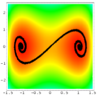
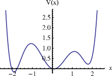
In our study of the LJ38 system, we carried out simulations of the stochastic dynamics of the clones but did not explicitly make the averages (18) that would yield the transition current. We argued in section III.2 that if one only looks for the reaction paths, then these averages are not necessary. In this appendix, we illustrate this claim on a simple 1d example that also allows us to discuss several aspects of the clone dynamics, namely the metastability, the finiteness of the clone population and the role of the initial condition.

We thus consider a system undergoing an underdamped Langevin dynamics

$$\dot{x}=v;\qquad\dot{v}=-\gamma v-m^{-1}V^{\prime}(x)+\sqrt{2\gamma kT/m}\,\eta$$ (35)

where $V(x)$ is a potential with two barriers, plotted in figure 9. We ran the clone dynamics for 2000 clones starting in the left well and carried out the averages (18).

Figure 9: Left: Plot of the potential $V(x)=x(-39+240x+15x^{2}-138x^{3}+20x^{5})/120$. Right: The green crosses are the position of the 2000 clones after a time $t=400$. The black arrows correspond to the averages (38) and indeed point tangentially to the reaction path. The color code and contour lines corresponds to the value of the Hamiltonian $H(x,v)=v^{2}/2+V(x)$

To do so, we constructed an approximate density from the positions and vectors $(x^{i},v^{i},u_{x}^{i},u_{v}^{i})$ of each of the ${\cal N}_{c}=2000$ clones:

$${\cal F}_{\rm num}(x,v,u_{x},u_{v})=\frac{1}{{\cal N}_{c}}\sum_{i=1}^{{\cal N}_{c}}\delta(x-x^{i})\delta(v-v^{i})\delta(u_{x}-u_{x}^{i})\delta(u_{v}-u_{v}^{i})$$ (36)

In principle, the $\delta$ should be Dirac functions but for practical purposes we replaced the one acting on the phase space coordinate by the bell-shaped function

$$\delta_{n}(x,v)=\frac{1}{Z}\exp\left(-\frac{1}{1-\frac{x^{2}+v^{2}}{w^{2}}}\right)\quad\text{if}\quad x^{2}+v^{2}<w^{2}\quad\text{and}\quad\delta_{n}(x,v)=0\quad\text{otherwise}$$ (37)

where $w=0.1$ and $Z$ is a normalization constant. Finally, using (36) and (37) in (18), we construct the transition current from the numerical data by computing

$${\bf J^{T}}(x,v)=\frac{1}{{\cal N}_{c}}\sum_{i=1}^{{\cal N}_{c}}{\bf u}^{i}\,\delta_{n}(x-x_{i},v-v_{i})$$ (38)

on a grid every $dx=dy=0.15$ and plot the resulting vector if its norm is larger than $10^{-3}$. For visualization purposes, we plot in the figures the vectors $5$ times longer than they really are.

We started a simulation with $2000$ clones in the left well, around $x=m_{1}\simeq-1.9$, with unitary vectors $(u_{x},u_{y})$ pointing at random. The temperature is set to $kT=0.09$ and the friction to $\gamma=1.5$ so that the mean first passage time across the barrier is HTB1990

$$T_{L\to C}\simeq\frac{2\pi}{\sqrt{\gamma^{2}/4+|V^{\prime\prime}(M_{1})|}-\gamma/2}\sqrt{\frac{|V^{\prime\prime}(M_{1})|}{V^{\prime\prime}(m_{1})}}e^{\frac{V(M_{1})-V(m_{1})}{kT}}\simeq 10^{7}$$ (39)

where $M_{1}$ is the first maximum of the potential $M_{1}\simeq-1$. The results of the simulation after a time $t=400$ are plotted in figure 9. The clones have already populated the barrier. foot5 As can be seen, the averages (38) along the reaction path are non-zero and result in vectors tangent to the reaction path, pointing toward the left well.

At later times, two processes take place, roughly on the same time scale. Firstly, more and more clones come back from the central well to the left one. Their vectors ${\bf u}$ are always tangent to their trajectories, but can be pointing toward the left or the central well with equal probability. Indeed, if $(p(t),q(t),{\bf u}(t))$ is a possible trajectory of the system, then so is $(p(t),q(t),-{\bf u}(t))$. As a result, the averages (38) may cancel out at large times, when the subpopulations of clones whose vectors ${\bf u}$ point toward the central and the left wells balance. This is how numerically the transition current is supposed to vanish at large time (another possibility being that all the clones leave a region of phase-space, because of finite population-size effects).

         

Figure 10: Left: $t=997$ the clones populate both barriers. The arrows average out along the reaction path between the left and central wells which have equilibrated, whereas the transition current is still present between the central and right wells Right: at $t=1590$ the clones only populate the reaction path between the central and right wells. Since the simulation had enough time to equilibrate the involved wells, the average (18) cancels out.

Secondly, some clones reach the barrier leading to the right well and duplicate, which results in populating the second reaction path. Since the clones did not have time to fall in the right well and cross back the barrier towards the central well with vectors ${\bf u}$ pointing in the opposite direction, the average (38) does not cancel along this reaction path.

Both effects can be seen in figure 10: the clones populate both barriers; the average (38) cancels out over the first barrier but not yet over the second one. This shows that the clone dynamics do locate the barriers and remain on the reaction paths even though the transition current may average out when the two wells separating a barrier equilibrate. This thus validates our approach to locate the reaction paths in the LJ38 system.

Note that if one wishes to study quantitatively the transition current, two modifications would need to be done to our algorithm. First, the initial condition should not be taken at random but constructed as proposed in section II.1. Second, rather than simulating all the clones in parallel while maintaining their population constant, it may be advantageous to run them sequentially, starting one run for every offspring of every clones, as is done for instance with the ‘Go with the winner’ methods. G2002 The constrain on the total population being fixed indeed affects the metastability of the clone dynamics and increases finite size effects. For instance, if there are ${\cal N}_{1}$ and ${\cal N}_{2}$ clones on the same reaction path, with vectors pointing in opposite directions, both populations grow exponentially with the same rate. Now, if the total population is kept constant, then the smallest sub-population disappears on average exponentially fast. Using a ‘Go with the winner’ method would palliate this drawback but would result in additional computational costs difficult to estimate beforehand.

References

- (1) D. Wales, Energy landscapes, Springer, 2003.
- (2) C. Dellago, P. Bolhuis, F. Csajka, D. Chandler, J. Chem. Phys. 108 (1998) 1964.
- (3) P. Bolhuis, D. Chandler, C. Dellago, P. Geissler, Annu. Rev. Phys. Chem. 53 (2002) 291.
- (4) T. Van Erp, P. Bolhuis, J. Comp. Phys. 205 (2005) 157.
- (5) See, for example: M Iannuzzi, A Laio, and M Parrinello, Phys. Rev. Lett. 90, 238302 (2003)
- (6) C. Valeriani, R. Allen, M. Morelli, D. Frenkel, P. ten Wolde, J. Chem. Phys. 127 (2007) 114109.
- (7) R. Allen, C. Valeriani, P. ten Wolde, J. Phys.: Condens. Matter 21 463102.
- (8) N. Mousseau, G. Barkema, Phys. Rev. E 57 (1998) 2419.
- (9) L. Munro, D. Wales, Phys. Rev. B 59 (1999) 3969.
- (10) G. Henkelman, H. Jónsson, J. Chem. Phys. 111 (1999) 7010.
- (11) S. Tănase-Nicola, J. Kurchan, J. Stat. Phys. 116 (2004) 1201.
- (12) J. Tailleur, S. Tănase-Nicola, J. Kurchan, J. Stat. Phys. 122 (2006) 557.
- (13) In a mathematical language, this amounts to embed the evolution of in a larger space and to later recover it through the projection (18).
- (14) J. Tailleur, J. Kurchan, Nature Phys. 3 (2007) 203.
- (15) S. Tănase-Nicola, J. Kurchan, Phys. Rev. Lett. 91 (2003) 188302.
- (16) H. Risken, The Fokker-Planck equation: Methods of solution and applications, Springer, 1989.
- (17) P. Hänggi, P. Talkner, M. Borkovec, Rev. Mod. Phys. 62 (1990) 251.
- (18) C. Gardiner, Handbook of stochastic methods, Springer Berlin, 1985.
- (19) G. Adjanor, M. Athènes, F. Calvo, Eur. Phys. J. B 53 (2006) 47.
- (20) Note however that the width of the clones distribution in the configuration space is of order TTK2006 so that for very large friction, these clouds start to cover several barriers at the same time and their dynamics can then change.
- (21) M. Athènes, G. Adjanor, J. Chem. Phys. 129 (2008) 024116.
- (22) M. El Makrini, B. Jourdain, T. Lelièvre, Diffusion Monte Carlo method: Numerical analysis in a simple case, ESAIM, Math. Model. Numer. Anal. 41 (2007) 189.
- (23) W. Cochran, Sampling techniques, Wiley India Pvt. Ltd., 2007.
- (24) A. Mossa, C. Clementi, Phys. Rev. E 75 (2007) 46707.
- (25) J. Doye, M. Miller, D. Wales, J. Chem. Phys. 111 (1999) 8417.
- (26) The vanishing of the current on a given branch appears usually in the program as a depopulation of clones in that region, but it can also be that their vectors are in counter-phase, so that their contribution to the current vanishes.
- (27) J. Doye, M. Miller, D. Wales, J. Chem. Phys. 110 (1999) 6896.
- (28) J. Neirotti, F. Calvo, D. Freeman, J. Doll, J. Chem. Phys. 112 (2000) 10340.
- (29) F. Calvo, J. Neirotti, D. Freeman, J. Doll, J. Chem. Phys. 112 (2000) 10350.
- (30) V. Mandelshtam, P. Frantsuzov, J. Chem. Phys. 124 (2006) 204511.
- (31) T. Bogdan, D. Wales, F. Calvo, J. Chem. Phys. 124 (2006) 044102.
- (32) P. Poulain, F. Calvo, R. Antoine, M. Broyer, P. Dugourd, Phys. Rev. E 73 (2006) 056704.
- (33) T. Miller, C. Predescu, Sampling diffusive transition paths, J. of Chem. Phys. 126 (2007) 144102.
- (34) M. Athènes, M.-C.. Marinica, J. Comput. Phys. 229 (2010) 7129.
- (35) D. Wales, Discrete path sampling, Mol. Phys. 100 (2002) 3285.
- (36) D. Wales, Mol. Phys. 102 (2004) 891.
- (37) D. J. Wales, J. Chem. Phys. 124 (2006) 234110.
- (38) S. Trygubenko, D. Wales, J. Chem. Phys. 124 (2006) 234110.
- (39) C. Dellago, P. Bolhuis, D. Chandler, J. Chem. Phys. 108 (1998) 9236.
- (40) P. Steinhardt, D. Nelson, M. Ronchetti, Phys. Rev. Lett. 47 (1981) 1297.
- (41) P. Steinhardt, D. Nelson, M. Ronchetti, Phys. Rev.B 28 (1983) 784.
- (42) Note that whereas some authors restrict the sum over bonds connecting atoms of the inner core, MF2006 ; ZCL2007 we include all the bonds in our definition.
- (43) L. Zhan, J. Z. Y. Chen, W. Liu, J. Chem. Phys. 127 (2007) 141101.
- (44) E. Sanz , C. Valeriani, D. Frenkel, M. Dijkstra, Phys. Rev. Lett. 99 (2007) 055501.
- (45) B. Peters, J. Chem. Phys. 131, 244103 (2009).
- (46) P. Geiger, C. Dellago, Chem. Phys. 375 (2010) 309.
- (47) Note that with standard Langevin simulations of the same duration, the probability that none of the 2000 clones has crossed the barrier is more than 90%.
- (48) P. Grassberger, Comp. Phys. Comm. 147 (2002) 64.