Abstract

Weakly Interacting Massive Particles (WIMPs) are one of the leading candidates for Dark Matter. So far the usual procedure for constraining the WIMP–nucleon cross sections in direct Dark Matter detection experiments have been to fit the predicted event rate based on some model(s) of the Galactic halo and of WIMPs to experimental data. One has to assume whether the spin–independent (SI) or the spin–dependent (SD) WIMP–nucleus interaction dominates, and results of such data analyses are also expressed as functions of the as yet unknown WIMP mass. In this article, I introduce methods for extracting information on the WIMP–nucleon cross sections by considering a general combination of the SI and SD interactions. Neither prior knowledge about the local density and the velocity distribution of halo WIMPs nor about their mass is needed. Assuming that an exponential–like shape of the recoil spectrum is confirmed from experimental data, the required information are only the measured recoil energies (in low energy ranges) and the number of events in the first energy bin from two or more experiments.

1 Introduction

Astronomical observations and measurements indicate that more than 80% of all matter in the Universe is dark (i.e., interacts at most very weakly with electromagnetic radiation and ordinary matter). The dominant component of this cosmological Dark Matter must be due to some yet to be discovered, non–baryonic particles. Weakly Interacting Massive Particles (WIMPs) $\chi$ arising in several extensions of the Standard Model of electroweak interactions are one of the leading candidates for Dark Matter. WIMPs are stable particles with masses roughly between 10 GeV and a few TeV and interact with ordinary matter only weakly (for reviews, see Refs. [1, 2]).

Currently, the most promising method to detect different WIMP candidates is the direct detection of the recoil energy deposited in a low–background underground detector by elastic scattering of ambient WIMPs off target nuclei [3, 4]. The basic expression for the differential event rate for elastic WIMP–nucleus scattering is given by [1]:

$$\frac{dR}{dQ}=\left(\frac{\rho_{0}\sigma_{0}}{2m_{\chi}m_{\rm r,N}^{2}}\right)F^{2}(Q)\int_{v_{\rm min}}^{v_{\rm max}}\left[\frac{f_{1}(v)}{v}\right]dv~{}\!.$$ (1)

Here $R$ is the direct detection event rate, i.e., the number of events per unit time and unit mass of detector material, $Q$ is the energy deposited in the detector, $\rho_{0}$ is the WIMP density near the Earth, $\sigma_{0}$ is the total cross section ignoring the form factor suppression and $F(Q)$ is the elastic nuclear form factor, $f_{1}(v)$ is the one–dimensional velocity distribution function of the WIMPs impinging on the detector, $v$ is the absolute value of the WIMP velocity in the laboratory frame. The reduced mass $m_{\rm r,N}$ is defined by

$$m_{\rm r,N}\equiv\frac{m_{\chi}m_{\rm N}}{m_{\chi}+m_{\rm N}}~{}\!,$$ (2)

where $m_{\chi}$ is the WIMP mass and $m_{\rm N}$ that of the target nucleus. Finally, $v_{\rm min}$ is the minimal incoming velocity of incident WIMPs that can deposit the energy $Q$ in the detector:

$$v_{\rm min}=\alpha\sqrt{Q}~{}\!,$$ (3)

with the transformation constant

$$\alpha\equiv\sqrt{\frac{m_{\rm N}}{2m_{\rm r,N}^{2}}}~{}\!,$$ (4)

and $v_{\rm max}$ is the maximal WIMP velocity in the Earth’s reference frame, which is related to the escape velocity from our Galaxy at the position of the Solar system, $v_{\rm esc}~{}\>\raisebox{-3.01385pt}{$\stackrel{{\scriptstyle\textstyle>}}{{\sim}}$}\>~{}600$ km/s.

1.1 WIMP–nucleus cross section

The total WIMP–nucleus cross section $\sigma_{0}$ in Eq. (1) depends on the nature of WIMP couplings on nucleons. Generally, for non–relativistic WIMPs, one can distinguish spin–independent (SI) and spin–dependent (SD) couplings.

1.1.1 Spin–independent couplings

Through e.g., squark and Higgs exchanges with quarks, WIMPs could have a “scalar” interaction with nuclei. The total cross section for the SI scalar interaction can be expressed as [1, 2]

$$\sigma_{0}^{\rm SI}=\left(\frac{4}{\pi}\right)m_{\rm r,N}^{2}\Big{[}Zf_{\rm p}+(A-Z)f_{\rm n}\Big{]}^{2}~{}\!.$$ (6)

Here $m_{\rm r,N}$ is the reduced mass defined in Eq. (2), $Z$ is the atomic number of the target nucleus, i.e., the number of protons, $A$ is the atomic mass number, $A-Z$ is then the number of neutrons, $f_{\rm(p,n)}$ are the effective scalar couplings of WIMPs on protons p and on neutrons n, respectively. Here we have to sum over the couplings on each nucleon before squaring because the wavelength associated with the momentum transfer is comparable to or larger than the size of the nucleus, the so–called “coherence effect”.

In addition, for the lightest supersymmetric neutralino, and for all WIMPs which interact primarily through Higgs exchange, the scalar couplings are approximately the same on protons and on neutrons [5]:

$$f_{\rm n}\simeq f_{\rm p}~{}\!.$$ (7)

The “pointlike” cross section $\sigma_{0}^{\rm SI}$ in Eq. (6) can thus be written as

$$\sigma_{0}^{\rm SI}\simeq\left(\frac{4}{\pi}\right)m_{\rm r,N}^{2}A^{2}|f_{\rm p}|^{2}=A^{2}\left(\frac{m_{\rm r,N}}{m_{\rm r,p}}\right)^{2}\sigma_{\chi{\rm p}}^{\rm SI}~{}\!,$$ (8)

where $m_{\rm r,p}$ is the reduced mass of the WIMP mass $m_{\chi}$ and the proton mass $m_{\rm p}$, and

$$\sigma_{\chi{\rm p}}^{\rm SI}=\left(\frac{4}{\pi}\right)m_{\rm r,p}^{2}|f_{\rm p}|^{2}$$ (9)

is the SI WIMP–nucleon cross section. The tiny mass difference between a proton and a neutron has been neglected.

1.1.2 Spin–dependent couplings

Through e.g., squark and Z boson exchanges with quarks, WIMPs could also couple to the spin of target nuclei, an “axial–vector” (spin–spin) interaction. The SD WIMP–nucleus cross section can be expressed as [1, 2]:

$$\sigma_{0}^{\rm SD}=\left(\frac{32}{\pi}\right)G_{F}^{2}~{}\!m_{\rm r,N}^{2}\left(\frac{J+1}{J}\right)\Big{[}\langle{\textstyle{S_{\rm p}}}\rangle a_{\rm p}+\langle{\textstyle{S_{\rm n}}}\rangle a_{\rm n}\Big{]}^{2}~{}\!.$$ (10)

Here $G_{F}$ is the Fermi constant, $J$ is the total spin of the target nucleus, $\langle{\textstyle{S_{\rm(p,n)}}}\rangle$ are the expectation values of the proton and neutron group spins, and $a_{\rm(p,n)}$ are the effective SD WIMP couplings on protons and on neutrons.

For the SD WIMP–nucleus interaction, it is usually assumed that only unpaired nucleons contribute significantly to the total cross section, as the spins of the nucleons in a nucleus are systematically anti–aligned. Under the “odd–group” assumption, the SD WIMP–nucleus cross section can be reduced to

$$\sigma_{0}^{\rm SD}=\left(\frac{32}{\pi}\right)G_{F}^{2}~{}\!m_{\rm r,N}^{2}\left(\frac{J+1}{J}\right)\langle{\textstyle{S_{\rm(p,n)}}}\rangle^{2}|a_{\rm(p,n)}|^{2}~{}\!.$$ (11)

Since for a proton or a neutron $J=\frac{1}{2}$ and $\langle{\textstyle{S_{\rm p}}}\rangle$ or $\langle{\textstyle{S_{\rm n}}}\rangle=\frac{1}{2}$, the SD WIMP cross section on protons or on neutrons can be given as

$$\sigma_{\chi{\rm(p,n)}}^{\rm SD}=\left(\frac{24}{\pi}\right)G_{F}^{2}~{}\!m_{\rm r,(p,n)}^{2}|a_{\rm(p,n)}|^{2}~{}\!.$$ (12)

Isotope	$Z$	$J$	$\langle{\textstyle{S_{\rm p}}}\rangle$	$\langle{\textstyle{S_{\rm n}}}\rangle$	$-\langle{\textstyle{S_{\rm p}}}\rangle/\langle{\textstyle{S_{\rm n}}}\rangle$	$\langle{\textstyle{S_{\rm n}}}\rangle/\langle{\textstyle{S_{\rm p}}}\rangle$	Natural abundance (%)
${}^{19}{\rm F}$	9	1/2	0.441	$-$0.109	4.05	$-$0.25	100
${}^{23}{\rm Na}$	11	3/2	0.248	0.020	$-$12.40	0.08	100
${}^{35}{\rm Cl}$	17	3/2	$-$0.059	$-$0.011	$-$5.36	0.19	76
${}^{37}{\rm Cl}$	17	3/2	$-$0.058	0.050	1.16	$-$0.86	24
${}^{73}{\rm Ge}$	32	9/2	0.030	0.378	$-$0.08	12.6	7.8 / 86 (HDMS) [9]
${}^{127}{\rm I}$	53	5/2	0.309	0.075	$-$4.12	0.24	100
${}^{129}{\rm Xe}$	54	1/2	0.028	0.359	$-$0.08	12.8	26
${}^{131}{\rm Xe}$	54	3/2	$-$0.009	$-$0.227	$-$0.04	25.2	21

Table 1: List of the relevant spin values of the nuclei used for simulations presented in this paper. More details can be found in e.g., Refs. [1, 6, 7, 8].

Moreover, once the upper and/or lower limits on the WIMP–nucleon cross sections have been estimated by Eq. (12), it has been shown that, for a particular WIMP mass, one can use the following inequality to give constraints on the SD WIMP–nucleon couplings on the $a_{\rm p}-a_{\rm n}$ plane [6, 10, 8]:

$$\left(\frac{a_{\rm p}}{\sqrt{\sigma_{\chi{\rm p}}^{\rm SD,upper}}}\pm\frac{a_{\rm n}}{\sqrt{\sigma_{\chi{\rm n}}^{\rm SD,upper}}}\right)^{2}\leq\frac{\pi}{24G_{F}^{2}m_{\rm r,p}^{2}}\leq\left(\frac{a_{\rm p}}{\sqrt{\sigma_{\chi{\rm p}}^{\rm SD,lower}}}\pm\frac{a_{\rm n}}{\sqrt{\sigma_{\chi{\rm n}}^{\rm SD,lower}}}\right)^{2}~{}\!.$$ (13)

Here $\sigma_{\chi({\rm p,n})}^{\rm SD,(upper,lower)}$ are the upper/lower limits on the SD WIMP–proton/neutron cross sections, respectively, and the “$\pm$” sign in the parenthesis is the same as that of the $\langle{\textstyle{S_{\rm n}}}\rangle/\langle{\textstyle{S_{\rm p}}}\rangle$ ratio. So far the best constraint on the SD WIMP–proton coupling comes from the NAIAD [11], KIMS [12], SIMPLE [13], PICASSO [14], and COUPP [15] experiments: $|a_{\rm p}|~{}\>\raisebox{-3.01385pt}{$\stackrel{{\scriptstyle\textstyle<}}{{\sim}}$}\>~{}0.4$ (for a WIMP mass of 50 GeV$/c^{2}$) [13], whereas the best one on the SD WIMP–neutron coupling comes from the CDMS-II [16], XENON10 [17], and ZEPLIN-III [18] experiments: $|a_{\rm n}|~{}\>\raisebox{-3.01385pt}{$\stackrel{{\scriptstyle\textstyle<}}{{\sim}}$}\>~{}0.2$ (for a WIMP mass of 50 GeV$/c^{2}$) [13]. On the other hand, the relative strength of two couplings for neutralino WIMPs has been calculated as [19]

$$0.55<\left|\frac{a_{\rm n}}{a_{\rm p}}\right|<0.8~{}\!.$$ (14)

Remind that the above conventional data analyses are independent of models of WIMP–nucleon couplings, but they do depend on the model of the Galactic halo through the use of the local WIMP density, $\rho_{0}$, and the velocity distribution of incident WIMPs, $f_{1}(v)$. Additionally, the results depend also strongly on the as yet unknown WIMP mass (see e.g., Refs. [10, 7, 8]).

1.1.3 Comparison of the SI and SD interactions

As discussed above, WIMPs could have both SI and SD interactions with target nuclei. Thus the WIMP–nucleus cross section $\sigma_{0}$ in Eq. (1) should be a combination of the SI cross section $\sigma_{0}^{\rm SI}$ in Eq. (6) and the SD cross section $\sigma_{0}^{\rm SD}$ in Eq. (10). However, due to the coherence effect with the entire nucleus shown in Eq. (8), the cross section for scalar interaction scales approximately as the square of the atomic mass number of the target nucleus. Hence, in most supersymmetric models, the SI cross section for nuclei with $A~{}\>\raisebox{-3.01385pt}{$\stackrel{{\scriptstyle\textstyle>}}{{\sim}}$}\>~{}30$ dominates over the SD one [1, 2]. Nevertheless, as discussed in Refs. [21, 22, 23], in Universal Extra Dimension (UED) models, the SD WIMP interaction with nucleus is less suppressed and could be compatible or even larger than the SI one.

1.2 Nuclear form factor

1.2.1 For the spin–independent cross section

For the SI cross section, there are some analytic forms for the elastic nuclear form factor. The simplest one is the exponential form factor, first introduced by Ahlen et al. [24] and Freese et al. [25]:

$$F_{\rm SI}^{2}(Q)=e^{-Q/Q_{0}}~{}\!.$$ (15)

Here $Q$ is the recoil energy transferred from the incident WIMP to the target nucleus,

$$Q_{0}=\frac{1.5}{m_{\rm N}R_{0}^{2}}$$ (16)

is the nuclear coherence energy and

$$R_{0}=\left[0.3+0.91\left(\frac{m_{\rm N}}{\rm GeV}\right)^{1/3}\right]~{}{\rm fm}$$ (17)

is the radius of the nucleus. The exponential form factor implies a Gaussian form of the radial density profile of the nucleus. This Gaussian density profile is simple, but not very realistic. Engel has therefore suggested to use the following one [26], which derives from the nuclear density profile obtained by convolving a constant nuclear density with a gaussian one [27], and is similar to the numerical form factor derived from the Woods–Saxon nuclear density profile [1, 2],

$$F_{\rm SI}^{2}(Q)=\left[\frac{3j_{1}(qR_{1})}{qR_{1}}\right]^{2}e^{-(qs)^{2}}~{}\!.$$ (18)

Here $j_{1}(x)$ is a spherical Bessel function,

$$q=\sqrt{2m_{\rm N}Q}$$ (19)

is the transferred 3-momentum,

$$R_{1}=\sqrt{R_{A}^{2}-5s^{2}}$$ (20)

is the effective nuclear radius with

$$R_{A}\simeq 1.2~{}\!A^{1/3}~{}{\rm fm},$$ (24)

and

$$s\simeq 1~{}{\rm fm}$$ (25)

is the nuclear skin thickness.

1.2.2 For the spin–dependent cross section

For the SD cross section, the form factor is different from nucleus to nucleus and no simple analytic form can provide a very good approximation. Generally, the form factor for the SD cross section can be expressed as [4, 1]

$$F_{\rm SD}^{2}(Q)=\frac{S(q)}{S(0)}~{}\!.$$ (26)

Here the “spin structure” function $S(q)$ depends generally on the SD WIMP–nucleon couplings:

$$S(q)=a_{0}^{2}S_{00}(q)+a_{1}^{2}S_{11}(q)+a_{0}a_{1}S_{01}(q)~{}\!,$$ (27)

with the isoscalar and isovector coefficients:

$$a_{0}=a_{\rm p}+a_{\rm n}~{}\!,~{}~{}~{}~{}~{}~{}~{}~{}~{}~{}~{}~{}~{}~{}~{}~{}~{}~{}~{}~{}a_{1}=a_{\rm p}-a_{\rm n}~{}\!,$$ (28)

and $S_{00}$, $S_{11}$, and $S_{01}$ are the isoscalar, isovector and interference contributions to $S(q)$, respectively.

However, Klapdor-Kleingrothaus et al. have used the following form factor for the SD cross section [29], introduced by Lewin and Smith with the so–called “thin–shell” approximation [4]:

$$F_{\rm SD}^{2}(Q) = \left\{\begin{array}[]{l l l}j_{0}^{2}(qR_{1})~{}\!,&{}{}{}{}{}{}{}{}&{\rm for}~{}qR_{1}\leq 2.55~{}{\rm or}~{}qR_{1}\geq 4.5~{}\!,\\ {\rm const.}\simeq 0.047~{}\!,&&{\rm for}~{}2.55\leq qR_{1}\leq 4.5~{}\!.\end{array}\right.$$ (31)

1.2.3 Zero momentum transfer approximation

For our simulations presented in this article, we will use the form factors given by Eqs. (18) and (31) for the SI and SD cross sections, respectively. However, it will be seen later that, since one would only have to estimate values of the form factors at the lowest energy ranges ( $\stackrel{{\scriptstyle\textstyle<}}{{\sim}}$  20 keV for some currently running and projected experiments), we could practically use the “zero momentum transfer” approximation:

$$F^{2}(Q\simeq 0)\simeq 1$$ (32)

in the methods introduced in this article.

1.3 Motivation

So far the usual procedure for estimating the (exclusion limits of the) WIMP–nucleon cross sections in direct Dark Matter detection experiments have been to fit the predicted event rate, $dR/dQ$ in Eq. (1), based on some model(s) of the Galactic halo from cosmology and of WIMPs from particle physics to experimental data. Meanwhile, one has to assume whether the SI or the SD WIMP–nucleus interaction dominates. However, WIMPs should in general have both interactions with target nuclei. Moreover, as mentioned above, although in most models with neutralino WIMPs as the best motivated candidate for Dark Matter, the theoretical predicted SI WIMP–nucleus cross section should be (much) larger than the SD one [5], Bertone et al. have shown that another Dark Matter candidate, the lightest Kaluza–Klein particle (LKP) arising in the Universal Extra Dimension (UED) models, has a relatively larger SD cross section, or, equivalently, a larger $\sigma_{\chi({\rm p,n})}^{\rm SD}$ to $\sigma_{\chi{\rm p}}^{\rm SI}$ ratio [21]. Hence, for determining the nature of Dark Matter particles and distinguishing them between e.g., the lightest neutralino in supersymmetric models and the lightest Kaluza–Klein particles in models with Universal Extra Dimensions, estimates of both SI and SD cross sections, or, at least an estimate of the ratio between these two cross sections, in direct Dark Matter detection experiments is essential.

On the other hand, as shown in our earlier work [30, 31] that one can determine the WIMP mass with direct Dark Matter detection experiments without a prior knowledge of the WIMP–nucleus cross section nor assumptions about the local density and the velocity distribution function of halo WIMPs. It is therefore important to investigate methods for, conversely, extracting information on the WIMP–nucleon cross sections from experimental data without knowing the WIMP mass.

The remainder of this article is organized as follows. In Secs. 2 and 3 I will show how to determine ratios of WIMP–nucleon couplings/cross sections once positive signals have been observed. Both the case that the SD WIMP interaction dominates (in Sec. 2) and that of a general combination of the SI and SD cross sections (in Sec. 3) will be considered. In Sec. 4 I will extend the data analysis procedure to the estimates of ratios between the SI WIMP scalar/vector couplings on protons and on neutrons. I conclude in Sec. 5. Some technical details for the data analysis will be given in an appendix.

2 Only a dominant SD WIMP–nucleus cross section

In this section I consider at first the case that the SD WIMP–nucleus interaction dominates over the SI one and derive the expression for determining the ratio between two SD WIMP–nucleon couplings.

2.1 General expression

By using a time–averaged recoil spectrum, and assuming that no directional information exists, the normalized one–dimensional velocity distribution function of halo WIMPs, $f_{1}(v)$, has been solved from Eq. (1) analytically [32] and, consequently, its generalized moments can be estimated by [32, 31]

$$\langle{\textstyle{v^{n}}}\rangle(v(Q_{\rm min}),v(Q_{\rm max})) = \int_{v(Q_{\rm min})}^{v(Q_{\rm max})}v^{n}f_{1}(v)~{}\!dv$$ (33)

$$= \alpha^{n}\left[\frac{2Q_{\rm min}^{(n+1)/2}r(Q_{\rm min})/F^{2}(Q_{\rm min})+(n+1)I_{n}(Q_{\rm min},Q_{\rm max})}{2Q_{\rm min}^{1/2}r(Q_{\rm min})/F^{2}(Q_{\rm min})+I_{0}(Q_{\rm min},Q_{\rm max})}\right]~{}\!.$$

Here $v(Q)=\alpha\sqrt{Q}$, $Q_{\rm(min,max)}$ are the experimental minimal and maximal cut–off energies of the data set, respectively,

$$r(Q_{\rm min})\equiv\left(\frac{dR}{dQ}\right)_{{\rm expt},~{}\!Q=Q_{\rm min}}$$ (34)

is an estimated value of the measured recoil spectrum $(dR/dQ)_{\rm expt}$ (before normalized by an experimental exposure $\cal E$) at $Q=Q_{\rm min}$, and $I_{n}(Q_{\rm min},Q_{\rm max})$ can be estimated through the sum:

$$I_{n}(Q_{\rm min},Q_{\rm max})=\sum_{a=1}^{N_{\rm tot}}\frac{Q_{a}^{(n-1)/2}}{F^{2}(Q_{a})}~{}\!,$$ (35)

where the sum runs over all events in the data set that satisfy $Q_{a}\in[Q_{\rm min},Q_{\rm max}]$ and $N_{\rm tot}$ is the number of such events.

Now, since the integral on the right–hand side of Eq. (1) is just the minus–first moment of the velocity distribution function, $\langle{\textstyle{v^{-1}}}\rangle$, which can be estimated by Eq. (33), by setting $Q=Q_{\rm min}$ and using the definition (4) of $\alpha$, one can obtain straightforwardly that

$$\rho_{0}\sigma_{0}=\left(\frac{1}{{\cal E}}\right)m_{\chi}m_{\rm r,N}\sqrt{\frac{m_{\rm N}}{2}}\left[\frac{2Q_{\rm min}^{1/2}r(Q_{\rm min})}{F^{2}(Q_{\rm min})}+I_{0}\right]~{}\!.$$ (36)

Then, in order to avoid the uncertainty of $\rho_{0}$ (of a factor of $\sim 2$ [1]), one can combine two experimental data sets with different target nuclei, $X$ and $Y$, to eliminate $\rho_{0}$ in Eq. (36) and thus obtain the following expression for the ratio between the WIMP cross section on nuclei $X$ and $Y$:

$$\frac{\sigma_{0,X}}{\sigma_{0,Y}}=\frac{m_{{\rm r},X}}{m_{{\rm r},Y}}\sqrt{\frac{m_{X}}{m_{Y}}}\left(\frac{{\cal R}_{\sigma,X}}{{\cal R}_{\sigma,Y}}\right)~{}\!,$$ (37)

where $m_{{\rm r},(X,Y)}$ are the reduced masses of the WIMP mass and the masses of target nucleus, $m_{(X,Y)}$, and I have defined

$${\cal R}_{\sigma,X}\equiv\frac{1}{{\cal E}_{X}}\left[\frac{2Q_{{\rm min},X}^{1/2}r_{X}(Q_{{\rm min},X})}{F_{X}^{2}(Q_{{\rm min},X})}+I_{0,X}\right]~{}\!,$$ (38)

and similar for ${\cal R}_{\sigma,Y}$; $F_{(X,Y)}(Q)$ here are the form factors of the nucleus $X$ and $Y$, $r_{(X,Y)}(Q_{{\rm min},(X,Y)})$ refer to the counting rates for the target $X$ and $Y$ at the respective lowest recoil energies included in the analysis, and ${\cal E}_{(X,Y)}$ are the experimental exposures with the target $X$ and $Y$. The emphasize here is that Eq. (37) can be used once positive signals are observed in two (or more) experiments; information on the local WIMP density $\rho_{0}$ and on the velocity distribution function of halo WIMPs, $f_{1}(v)$, are not necessary.

Substituting the expression (10) for $\sigma_{0}^{\rm SD}$ into Eq. (37) and using the definition (4) of $\alpha$ for both target nuclei, one can solve the ratio between two SD WIMP–nucleon couplings analytically as [33]

$$\left(\frac{a_{\rm n}}{a_{\rm p}}\right)_{\pm,n}^{\rm SD}=-\frac{\langle{\textstyle{S_{\rm p}}}\rangle_{X}\pm\langle{\textstyle{S_{\rm p}}}\rangle_{Y}\left({\cal R}_{J,n,X}/{\cal R}_{J,n,Y}\right)}{\langle{\textstyle{S_{\rm n}}}\rangle_{X}\pm\langle{\textstyle{S_{\rm n}}}\rangle_{Y}\left({\cal R}_{J,n,X}/{\cal R}_{J,n,Y}\right)}~{}\!,$$ (39)

for $n\neq 0$. Here I have used the relation [31]:

$$\frac{\alpha_{X}}{\alpha_{Y}}=\frac{{\cal R}_{n,Y}}{{\cal R}_{n,X}}~{}\!,$$ (40)

and defined

$${\cal R}_{J,n,X}\equiv\left[\Bigg{(}\frac{J_{X}}{J_{X}+1}\Bigg{)}\frac{{\cal R}_{\sigma,X}}{{\cal R}_{n,X}}\right]^{1/2}~{}\!,$$ (41)

with ${\cal R}_{\sigma,X}$ defined in Eq. (38) and

$${\cal R}_{n,X}\equiv\left[\frac{2Q_{{\rm min},X}^{(n+1)/2}r_{X}(Q_{{\rm min},X})/F_{X}^{2}(Q_{{\rm min},X})+(n+1)I_{n,X}}{2Q_{{\rm min},X}^{1/2}r_{X}(Q_{{\rm min},X})/F_{X}^{2}(Q_{{\rm min},X})+I_{0,X}}\right]^{1/n}~{}\!;$$ (42)

${\cal R}_{J,n,Y}$ and ${\cal R}_{n,Y}$ can be defined analogously. Note that Eq. (39) is independent of the WIMP mass and can be used for estimating $a_{\rm n}/a_{\rm p}$ with measured recoil energies directly.

Because the couplings in Eq. (10) are squared, we have two solutions for $a_{\rm n}/a_{\rm p}$ here; if exact “theory” values for ${\cal R}_{J,n,(X,Y)}$ are taken, these solutions coincide for

$$\left(\frac{a_{\rm n}}{a_{\rm p}}\right)_{+,n}^{\rm SD}=\left(\frac{a_{\rm n}}{a_{\rm p}}\right)_{-,n}^{\rm SD}=\left\{\begin{array}[]{l l l}\displaystyle-\frac{\langle{\textstyle{S_{\rm p}}}\rangle_{X}}{\langle{\textstyle{S_{\rm n}}}\rangle_{X}}~{}\!,&{}{}{}{}{}{}{}{}&{\rm for}~{}{\cal R}_{J,n,X}=0~{}\!,\\ \\ \displaystyle-\frac{\langle{\textstyle{S_{\rm p}}}\rangle_{Y}}{\langle{\textstyle{S_{\rm n}}}\rangle_{Y}}~{}\!,&&{\rm for}~{}{\cal R}_{J,n,Y}=0~{}\!,\end{array}\right.$$ (43)

which depends only on properties of two used target nuclei (see Table 1). Moreover, it can be found from Eq. (39) that one of these two solutions has a pole at the middle of two intersections, which depends simply on the signs of $\langle{\textstyle{S_{\rm n}}}\rangle_{X}$ and $\langle{\textstyle{S_{\rm n}}}\rangle_{Y}$: since ${\cal R}_{J,n,X}$ and ${\cal R}_{J,n,Y}$ are always positive, if both $\langle{\textstyle{S_{\rm n}}}\rangle_{X}$ and $\langle{\textstyle{S_{\rm n}}}\rangle_{Y}$ are positive or negative, the “$-$ (minus)” solution $(a_{\rm n}/a_{\rm p})^{\rm SD}_{-,n}$ will diverge and the “$+$ (plus)” solution $(a_{\rm n}/a_{\rm p})^{\rm SD}_{+,n}$ will be the “inner” solution; in contrast, if the signs of $\langle{\textstyle{S_{\rm n}}}\rangle_{X}$ and $\langle{\textstyle{S_{\rm n}}}\rangle_{Y}$ are opposite, the “$-$ (minus)” solution $(a_{\rm n}/a_{\rm p})^{\rm SD}_{-,n}$ will be the “inner” solution (see Figs. 1).

By using the standard Gaussian error propagation, the statistical uncertainty on $\left(a_{\rm n}/a_{\rm p}\right)_{\pm,n}^{\rm SD}$ can be expressed as

$$\sigma\left(\left(\frac{a_{\rm n}}{a_{\rm p}}\right)_{\pm,n}^{\rm SD}\right) = \frac{\Big{|}\langle{\textstyle{S_{\rm p}}}\rangle_{Y}\langle{\textstyle{S_{\rm n}}}\rangle_{X}-\langle{\textstyle{S_{\rm p}}}\rangle_{X}\langle{\textstyle{S_{\rm n}}}\rangle_{Y}\Big{|}}{\Big{[}\langle{\textstyle{S_{\rm n}}}\rangle_{X}\pm\langle{\textstyle{S_{\rm n}}}\rangle_{Y}({\cal R}_{J,n,X}/{\cal R}_{J,n,Y})\Big{]}^{2}}\left(\frac{1}{2}\cdot\frac{{\cal R}_{J,n,X}}{{\cal R}_{J,n,Y}}\right)$$ (44)

$$~{}~{}\times\Bigg{\{}\sum_{i,j=1}^{3}\left[\frac{1}{{\cal R}_{n,X}}\left(\frac{\partial{\cal R}_{n,X}}{\partial c_{i,X}}\right)-\frac{1}{{\cal R}_{\sigma,X}}\left(\frac{\partial{\cal R}_{\sigma,X}}{\partial c_{i,X}}\right)\right]\Bigg{.}$$

$$~{}~{}~{}~{}~{}~{}~{}~{}~{}~{}~{}~{}~{}~{}~{}~{}\times\left[\frac{1}{{\cal R}_{n,X}}\left(\frac{\partial{\cal R}_{n,X}}{\partial c_{j,X}}\right)-\frac{1}{{\cal R}_{\sigma,X}}\left(\frac{\partial{\cal R}_{\sigma,X}}{\partial c_{j,X}}\right)\right]{\rm cov}(c_{i,X},c_{j,X})$$

$$~{}~{}~{}~{}~{}~{}~{}~{}~{}~{}~{}~{}\Bigg{.}+(X\longrightarrow Y)\Bigg{\}}^{1/2}~{}\!.$$

Here a short–hand notation for the six quantities on which the estimate of $(a_{\rm n}/a_{\rm p})_{\pm,n}^{\rm SD}$ depends has been introduced [31]:

$$c_{1,X}=I_{n,X}~{}\!,~{}~{}~{}~{}~{}~{}~{}~{}~{}~{}~{}~{}c_{2,X}=I_{0,X}~{}\!,~{}~{}~{}~{}~{}~{}~{}~{}~{}~{}~{}~{}c_{3,X}=r_{X}(Q_{{\rm min},X})~{}\!;$$ (45)

and similarly for the $c_{i,Y}$. Estimators for ${\rm cov}(c_{i},c_{j})$ and explicit expressions for the derivatives of ${\cal R}_{n,X}$ and ${\cal R}_{\sigma,X}$ with respect to $c_{i,X}$ will be given in the appendix. Note that ${\cal R}_{\sigma,(X,Y)}$ are actually independent of $c_{1,(X,Y)}=I_{n,(X,Y)}$, for $n\neq 0$.

In Figs. 1 I show the numerical results for a target combination of ${}^{73}{\rm Ge}$ and ${}^{37}{\rm Cl}$ with 5,000 experiments based on the Monte Carlo simulation. The theoretical predicted recoil spectrum for the shifted Maxwellian velocity distribution [1, 2, 32] with a Sun’s orbital velocity in the Galactic frame $v_{0}=220$ km/s, an Earth’s velocity in the Galactic frame $v_{\rm e}=1.05~{}\!v_{0}$, and a maximal cut–off velocity of the velocity distribution function $v_{\rm max}=700$ km/s, as well as the nuclear form factor given in Eq. (31) have been used. The experimental minimal and maximal cut–off energies have been set as $Q_{\rm min}=5$ keV and $Q_{\rm max}=100$ keV for both targets. Each experiment contains an expected number of 50 total events; the actual event number is Poisson–distributed around this expectation value. The input WIMP mass has been set as 100 GeV.

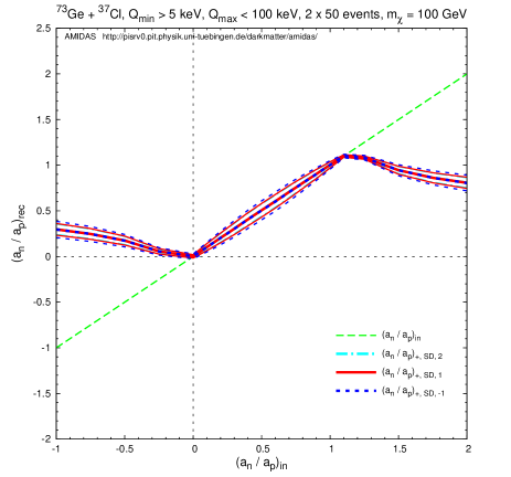
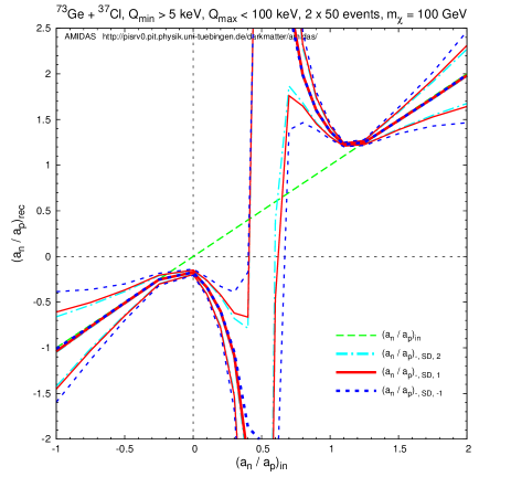
Figure 1: The reconstructed $a_{\rm n}/a_{\rm p}$ ratios estimated by Eq. (39) and the lower and upper bounds of their 1$\sigma$ statistical uncertainties estimated by Eq. (44) with $n=-1$ (dashed blue), 1 (solid red), and 2 (dash–dotted cyan) as functions of the input $a_{\rm n}/a_{\rm p}$ ratio. Here I show the “$+$ ($-$)” solutions in the left (right) frames separately. The theoretical predicted recoil spectrum for the shifted Maxwellian velocity distribution with $v_{0}=220$ km/s, $v_{\rm e}=1.05~{}\!v_{0}$, and $v_{\rm max}=700$ km/s as well as the nuclear form factor for the SD cross section given in Eq. (31) have been used. ${}^{73}{\rm Ge}$ and ${}^{37}{\rm Cl}$ have been chosen as two target nuclei. Each experiment contains 50 total events on average in the energy range between 5 and 100 keV. The input WIMP mass has been set as 100 GeV. See the text for further details.

As discussed above, since $\langle{\textstyle{S_{\rm n}}}\rangle_{{}^{73}{\rm Ge}}$ and $\langle{\textstyle{S_{\rm n}}}\rangle_{{}^{37}{\rm Cl}}$ have the same sign, the “$+$” solution shown in the left frame of Figs. 1 is the inner solution for the range of interest $0\leq a_{\rm n}/a_{\rm p}\leq 1$, while the “$-$” solution shown in the right frame diverges between $-\langle{\textstyle{S_{\rm p}}}\rangle_{{}^{73}{\rm Ge}}/\langle{\textstyle{S_{\rm n}}}\rangle_{{}^{73}{\rm Ge}}=-0.08$ and $-\langle{\textstyle{S_{\rm p}}}\rangle_{{}^{37}{\rm Cl}}/\langle{\textstyle{S_{\rm n}}}\rangle_{{}^{37}{\rm Cl}}=1.16$. Note here that, for practical use of analyzing real data, one might however not be able to make a choice from the “$+$” and “$-$” estimates given by Eq. (39), especially if they are close to the coincidences, e.g., around 1.16 or $-$0.08 here. For example, for a true $a_{\rm n}/a_{\rm p}=1.1$, one will get $(a_{\rm n}/a_{\rm p})_{+}^{\rm SD}\cong 1.1$ and $(a_{\rm n}/a_{\rm p})_{-}^{\rm SD}\cong 1.25$, the same results as for the case with a true $a_{\rm n}/a_{\rm p}=1.25$.

2.2 Reducing statistical uncertainty on $(a_{\rm n}/a_{\rm p})_{\pm,n}^{\rm SD}$

For estimating the statistical uncertainty on $(a_{\rm n}/a_{\rm p})_{\pm,n}^{\rm SD}$ by Eq. (44), one needs to estimate contributions from the counting rate at the threshold energy, $r(Q_{\rm min})$, from $I_{n}$ given in Eq. (35), and from the covariance between $r(Q_{\rm min})$ and $I_{n}$. From Eqs. (A9), (A10) and (A13) in the appendix, one can find a way to reduce these statistical uncertainties by estimating the counting rate, instead of at the experimental minimal cut–off energy, at the shifted point $Q_{s,1}$ (from the central point of the first bin, $Q_{1}$):

$$Q_{s,1}=Q_{1}+\frac{1}{k_{1}}\ln\left[\frac{\sinh(k_{1}b_{1}/2)}{k_{1}b_{1}/2}\right]~{}\!,$$ (46)

where $k_{1}$ is the logarithmic slope of the reconstructed recoil spectrum in the first $Q-$bin and $b_{1}$ is the bin width. Then, according to Eq. (A9), the measured recoil spectrum at $Q=Q_{s,1}$ can be estimated by

$$r(Q_{s,1})=\left(\frac{dR}{dQ}\right)_{{\rm expt},~{}\!1,~{}\!Q=Q_{s,1}}=r_{1}=\frac{N_{1}}{b_{1}}~{}\!,$$ (47)

with the statistical uncertainty given as

$$\sigma^{2}(r(Q_{s,1}))=\sigma^{2}(r_{1})=\frac{N_{1}}{b_{1}^{2}}~{}\!,$$ (48)

where $N_{1}$ is the event number in the first bin.

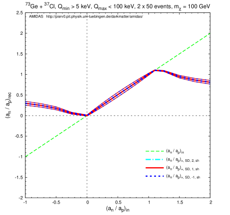
Figure 2: As in Figs. 1, except that we estimate $(a_{\rm n}/a_{\rm p})_{\pm,n}^{\rm SD}$ with the counting rates at the shifted points of the first $Q-$bin, $r_{(X,Y)}(Q_{s,1,(X,Y)})=r_{(X,Y),1}$.

In Figs. 2 I show the reconstructed $a_{\rm n}/a_{\rm p}$ ratios and the lower and upper bounds of their 1$\sigma$ statistical uncertainties with $n=-1$ (dashed blue), 1 (solid red), and 2 (dash–dotted cyan) estimated by Eq. (39) with the counting rates at the shifted points of the first $Q-$bin, $r_{(X,Y)}(Q_{s,1,(X,Y)})=r_{(X,Y),1}$ as functions of the input $a_{\rm n}/a_{\rm p}$ ratio. It can be seen that the statistical uncertainties on $(a_{\rm n}/a_{\rm p})_{\pm,n}^{\rm SD}$ estimated with different $n$ (namely with different moments of the WIMP velocity distribution) with $r_{(X,Y)}(Q_{s,1,(X,Y)})$ are clearly reduced and, interestingly, almost equal. Therefore, since

$${\cal R}_{J,-1,X}=\left[\left(\frac{J_{X}}{J_{X}+1}\right)\frac{2~{}\!r_{X}(Q_{s,1,X})}{{\cal E}_{X}F_{X}^{2}(Q_{s,1,X})}\right]^{1/2}~{}\!,$$ (49)

one would practically only need events in the lowest energy ranges ($\sim$ 20 events between 5 and 15 keV in our simulations) for estimating $a_{\rm n}/a_{\rm p}$. Consequently, one has to estimate the values of form factors only at $Q=Q_{s,1}$, and the zero momentum transfer approximation $F^{2}(Q\simeq 0))\simeq 1$ can be used. In fact, our simulation shows that a relatively higher threshold energy ($Q_{\rm min}\sim$ 10 keV and $Q_{s,1}\sim$ 14 keV) should not affect the reconstruction of $a_{\rm n}/a_{\rm p}$ significantly, especially for the first approximation with pretty few events and thus a large statistical uncertainty.

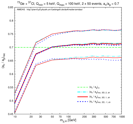
Figure 3: The reconstructed $a_{\rm n}/a_{\rm p}$ ratios estimated by Eq. (39) and the lower and upper bounds of their 1$\sigma$ statistical uncertainties with $n=-1$ (dashed blue), 1 (solid red), and 2 (dash–dotted cyan) as functions of the input WIMP mass $m_{\chi}$. Here we estimate with $r_{(X,Y)}(Q_{{\rm min},(X,Y)})$ (left) and $r_{(X,Y)}(Q_{s,1,(X,Y)})$ (right). The input $a_{\rm n}/a_{\rm p}$ ratio has been set as 0.7. The other parameters and notations are as in Figs. 1 and 2.

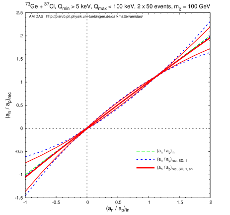
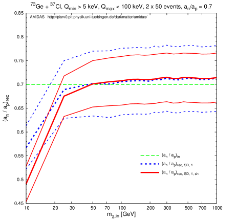
Figure 4: Left: the combined results of the “$+$” and “$-$” solutions estimated with $r_{(X,Y)}(Q_{{\rm min},(X,Y)})$ (dashed blue) shown in Figs. 1 and with $r_{(X,Y)}(Q_{s,1,(X,Y)})$ (solid red) in Figs. 2. Right: a comparison of the results shown in Figs. 3 estimated with $r_{(X,Y)}(Q_{{\rm min},(X,Y)})$ (dashed blue) and with with $r_{(X,Y)}(Q_{s,1,(X,Y)})$ (solid red). Only the results estimated with $n=1$ are shown here.

On the other hand, as mentioned above, the expression (39) for estimating the ratio between two SD WIMP–nucleon couplings is independent of the WIMP mass. In Figs. 3, I show the reconstructed $a_{\rm n}/a_{\rm p}$ ratio and the lower and upper bounds of their 1$\sigma$ statistical uncertainties as functions of the input WIMP mass $m_{\chi}$ for a fixed input $a_{\rm n}/a_{\rm p}=0.7$. We estimate with $r_{(X,Y)}(Q_{{\rm min},(X,Y)})$ and $r_{(X,Y)}(Q_{s,1,(X,Y)})$ in the left and right frames, respectively. It can be seen that, firstly, except the statistical uncertainty estimated with $r_{(X,Y)}(Q_{{\rm min},(X,Y)})$ and $n=-1$ (the dashed blue curves labeled as $(a_{\rm n}/a_{\rm p})_{\rm rec,~{}SD,~{}-1}$ in the left frame), for WIMP masses $m_{\chi}~{}\>\raisebox{-3.01385pt}{$\stackrel{{\scriptstyle\textstyle>}}{{\sim}}$}\>$ 50 GeV, the reconstructed $a_{\rm n}/a_{\rm p}$ ratio as well as the statistical uncertainty are (almost) independent of the WIMP mass; however, if WIMPs are (very) light ($m_{\chi}~{}\>\raisebox{-3.01385pt}{$\stackrel{{\scriptstyle\textstyle<}}{{\sim}}$}\>~{}25$ GeV), $a_{\rm n}/a_{\rm p}$ will be (strongly) underestimated, due to the non–zero threshold energies. Secondly, the statistical uncertainties on $a_{\rm n}/a_{\rm p}$ estimated with $r_{(X,Y)}(Q_{{\rm min},(X,Y)})$ and $r_{(X,Y)}(Q_{s,1,(X,Y)})$ are only 10% or even 7% combined with an $\sim$ 1.5% systematic deviation.

As a comparison, I show the combinations of the “$+$” and “$-$” solutions with $n=1$ shown in Figs. 1 and 2 together in the left frame of Figs. 4. In the right frame, I compare also the results with $n=1$ shown in Figs. 3. The $\sim 30\%$ (from 10% to 7%) reduction of the statistical uncertainty by estimating with $r_{(X,Y)}(Q_{s,1,(X,Y)})$ for $m_{\chi}~{}\>\raisebox{-3.01385pt}{$\stackrel{{\scriptstyle\textstyle>}}{{\sim}}$}\>~{}100$ GeV can be seen obviously.

Furthermore, considering the low natural abundances of ${}^{73}{\rm Ge}$ and ${}^{37}{\rm Cl}$ (see Table 1), in Figs. 5 we simulate with another combination of target nuclei: ${}^{19}{\rm F}$ and ${}^{127}{\rm I}$. As discussed in the previous subsection and shown in Figs. 1, 2, and 4, the inner solutions of $(a_{\rm n}/a_{\rm p})_{\pm,n}^{\rm SD}$ have a much smaller statistical uncertainties and the range of these inner solutions depends on the $-\langle{\textstyle{S_{\rm p}}}\rangle/\langle{\textstyle{S_{\rm n}}}\rangle$ values of our target nuclei. Hence, one benefit of using the combination of ${}^{19}{\rm F}$ and ${}^{127}{\rm I}$ is that one can estimate $(a_{\rm n}/a_{\rm p})_{\pm,n}^{\rm SD}$ in a much wilder range of interest: $|a_{\rm n}/a_{\rm p}|\leq 4$. Consequently, for the practical use of analyzing real data, one has therefore not to worry about making the choice from the “$+$” and “$-$” estimates, which is discussed at the end of the previous subsection; since $\langle{\textstyle{S_{\rm n}}}\rangle_{{}^{19}{\rm F}}$ and $\langle{\textstyle{S_{\rm n}}}\rangle_{{}^{127}{\rm I}}$ have different signs, we can just take the “$-$” solution in Eq. (39).

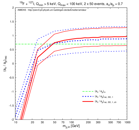
Figure 5: As in Figs. 4, except that ${}^{19}{\rm F}$ and ${}^{127}{\rm I}$ have been chosen as two target nuclei. Note that the scales used here are different from those in Figs. 4.

However, Figs. 5 show us also some drawbacks of the use of the ${}^{19}{\rm F}$ $+$ ${}^{127}{\rm I}$ combination. For WIMP masses $m_{\chi}~{}\>\raisebox{-3.01385pt}{$\stackrel{{\scriptstyle\textstyle>}}{{\sim}}$}\>~{}50$ GeV, $(a_{\rm n}/a_{\rm p})_{\pm,n}^{\rm SD}$ estimated with $r_{(X,Y)}(Q_{{\rm min},(X,Y)})$ (dashed blue) are $\sim$ 15% - 30% overestimated; whereas those estimated with $r_{(X,Y)}(Q_{s,1,(X,Y)})$ (solid red) are even worse: $\sim 36\%$ for $m_{\chi}\sim 1$ TeV. Moreover, the statistical uncertainties shown here become also much larger (of a factor of $\sim 3-5$) than those shown in Figs. 4. This enlargement of the statistical uncertainties is mainly caused by the larger value of the prefactor of $\sigma((a_{\rm n}/a_{\rm p})_{\pm,n}^{\rm SD})$ in Eq. (44). According to Table 1, the values of $\Big{|}\langle{\textstyle{S_{\rm p}}}\rangle_{Y}\langle{\textstyle{S_{\rm n}}}\rangle_{X}-\langle{\textstyle{S_{\rm p}}}\rangle_{X}\langle{\textstyle{S_{\rm n}}}\rangle_{Y}\Big{|}$ are $\sim$ 0.023 for the Ge $+$ Cl combination, but $\sim$ 0.067 for F $+$ I. Meanwhile, as shown in both Figs. 4 and 5, the statistical uncertainties are at the largest in the middle of two coincidence points and reduce as the input $a_{\rm n}/a_{\rm p}$ approaches to one of these two points. Since we set the input $a_{\rm n}/a_{\rm p}=0.7$ for simulations with different WIMP masses, comparing to the relative difference between 0.7 and the middle point of 1.16 and $-$0.08, i.e., 0.54, the relative difference between 0.7 and the middle point of 4.05 and $-$4.12, i.e., $-$0.035, is slightly smaller. This causes also a larger statistical uncertainty for the use of the F $+$ I combination. In contrast, for light WIMP masses ($m_{\chi}~{}\>\raisebox{-3.01385pt}{$\stackrel{{\scriptstyle\textstyle<}}{{\sim}}$}\>~{}50$ GeV), the two estimates with ${}^{19}{\rm F}$ and ${}^{127}{\rm I}$ shown in the right frame of Figs. 5 are much more underestimated than results shown in the right frame of Figs. 4.

3 Combination of the SI and SD cross sections

In this section I consider the general combination of the SI and SD WIMP–nucleus cross sections.

3.1 General expression

At first, by combining Eqs. (8), (10), and (12), we can find

$$\frac{\sigma_{0}^{\rm SD}}{\sigma_{0}^{\rm SI}}=\left(\frac{32}{\pi}\right)G_{F}^{2}~{}\!m_{\rm r,p}^{2}\Bigg{(}\frac{J+1}{J}\Bigg{)}\left[\frac{\langle{\textstyle{S_{\rm p}}}\rangle+\langle{\textstyle{S_{\rm n}}}\rangle(a_{\rm n}/a_{\rm p})}{A}\right]^{2}\frac{|a_{\rm p}|^{2}}{\sigma_{\chi{\rm p}}^{\rm SI}}={\cal C}_{\rm p}\left(\frac{\sigma_{\chi{\rm p}}^{\rm SD}}{\sigma_{\chi{\rm p}}^{\rm SI}}\right)~{}\!,$$ (50)

where I have defined

$${\cal C}_{\rm p}\equiv\frac{4}{3}\left(\frac{J+1}{J}\right)\left[\frac{\langle{\textstyle{S_{\rm p}}}\rangle+\langle{\textstyle{S_{\rm n}}}\rangle(a_{\rm n}/a_{\rm p})}{A}\right]^{2}~{}\!.$$ (51)

For the general combination of the SI and SD WIMP–nucleus cross sections, the expression (1) for the differential event rate should be modified to

$$\left(\frac{dR}{dQ}\right)_{\rm expt} = {\cal E}\left(\frac{\rho_{0}}{2m_{\chi}m_{\rm r,N}^{2}}\right)\bigg{[}\sigma_{0}^{\rm SI}F_{\rm SI}^{2}(Q)+\sigma_{0}^{\rm SD}F_{\rm SD}^{2}(Q)\bigg{]}\int_{v_{\rm min}}^{v_{\rm max}}\left[\frac{f_{1}(v)}{v}\right]dv$$ (52)

$$= {\cal E}A^{2}\!\left(\frac{\rho_{0}\sigma_{\chi{\rm p}}^{\rm SI}}{2m_{\chi}m_{\rm r,p}^{2}}\right)\!\!\left[F_{\rm SI}^{2}(Q)+\left(\frac{\sigma_{\chi{\rm p}}^{\rm SD}}{\sigma_{\chi{\rm p}}^{\rm SI}}\right){\cal C}_{\rm p}F_{\rm SD}^{2}(Q)\right]\int_{v_{\rm min}}^{v_{\rm max}}\left[\frac{f_{1}(v)}{v}\right]dv~{}\!,$$

where I have used Eq. (8) again. Then one can find straightforwardly that the integral above can be estimated by Eq. (33) with the following replacement:

$$F^{2}(Q_{\rm min})\to F^{\prime 2}(Q_{\rm min})\equiv F_{\rm SI}^{2}(Q_{\rm min})+\left(\sigma_{\chi{\rm p}}^{\rm SD}/\sigma_{\chi{\rm p}}^{\rm SI}\right){\cal C}_{\rm p}F_{\rm SD}^{2}(Q_{\rm min})~{}\!.$$ (53)

Hence, for this general case, Eq. (36) becomes to

$$\rho_{0}\left[A^{2}\left(\frac{m_{\rm r,N}}{m_{\rm r,p}}\right)^{2}\sigma_{\chi{\rm p}}^{\rm SI}\right]=\left(\frac{1}{{\cal E}}\right)m_{\chi}m_{\rm r,N}\sqrt{\frac{m_{\rm N}}{2}}\left[\frac{2Q_{\rm min}^{1/2}r(Q_{\rm min})}{F^{\prime 2}(Q_{\rm min})}+I_{0}\right]~{}\!,$$ (54)

where

$$I_{n}(Q_{\rm min},Q_{\rm max})=\sum_{a=1}^{N_{\rm tot}}\frac{Q_{a}^{(n-1)/2}}{F^{\prime 2}(Q_{a})}~{}\!.$$ (55)

Now by combining two targets $X$ and $Y$ and using the definition (4) of $\alpha$, the relation (40) between $\alpha_{X}/\alpha_{Y}$ with $n=-1$, as well as the expression (42) for ${\cal R}_{n,(X,Y)}$, one can obtain that

$$\frac{F_{{\rm SI},X}^{2}(Q_{{\rm min},X})+\left(\sigma_{\chi{\rm p}}^{\rm SD}/\sigma_{\chi{\rm p}}^{\rm SI}\right){\cal C}_{{\rm p},X}F_{{\rm SD},X}^{2}(Q_{{\rm min},X})}{F_{{\rm SI},Y}^{2}(Q_{{\rm min},Y})+\left(\sigma_{\chi{\rm p}}^{\rm SD}/\sigma_{\chi{\rm p}}^{\rm SI}\right){\cal C}_{{\rm p},Y}F_{{\rm SD},Y}^{2}(Q_{{\rm min},Y})}=\frac{{\cal R}_{m,X}}{{\cal R}_{m,Y}}~{}\!,$$ (56)

where I have assumed $m_{(X,Y)}\propto A_{(X,Y)}$ and defined

$${\cal R}_{m,X}\equiv\frac{r_{X}(Q_{{\rm min},X})}{{\cal E}_{X}m_{X}^{2}}~{}\!.$$ (57)

From Eq. (56), the ratio of the SD WIMP–proton cross section to the SI one can be solved analytically as [33]

$$\frac{\sigma_{\chi{\rm p}}^{\rm SD}}{\sigma_{\chi{\rm p}}^{\rm SI}}=\frac{F_{{\rm SI},Y}^{2}(Q_{{\rm min},Y})({\cal R}_{m,X}/{\cal R}_{m,Y})-F_{{\rm SI},X}^{2}(Q_{{\rm min},X})}{{\cal C}_{{\rm p},X}F_{{\rm SD},X}^{2}(Q_{{\rm min},X})-{\cal C}_{{\rm p},Y}F_{{\rm SD},Y}^{2}(Q_{{\rm min},Y})({\cal R}_{m,X}/{\cal R}_{m,Y})}~{}\!,$$ (58)

where ${\cal C}_{{\rm p},(X,Y)}$ have been defined in Eq. (51). Similarly, the ratio of the SD WIMP–neutron cross section to the SI one can be given analogously as [33]

$$\frac{\sigma_{\chi{\rm n}}^{\rm SD}}{\sigma_{\chi{\rm p}}^{\rm SI}}=\frac{F_{{\rm SI},Y}^{2}(Q_{{\rm min},Y})({\cal R}_{m,X}/{\cal R}_{m,Y})-F_{{\rm SI},X}^{2}(Q_{{\rm min},X})}{{\cal C}_{{\rm n},X}F_{{\rm SD},X}^{2}(Q_{{\rm min},X})-{\cal C}_{{\rm n},Y}F_{{\rm SD},Y}^{2}(Q_{{\rm min},Y})({\cal R}_{m,X}/{\cal R}_{m,Y})}~{}\!,$$ (59)

with the definition

$${\cal C}_{\rm n}\equiv\frac{4}{3}\Bigg{(}\frac{J+1}{J}\Bigg{)}\left[\frac{\langle{\textstyle{S_{\rm p}}}\rangle(a_{\rm p}/a_{\rm n})+\langle{\textstyle{S_{\rm n}}}\rangle}{A}\right]^{2}~{}\!.$$ (60)

The emphasize here is that one can use expressions (58) and (59) to estimate $\sigma_{\chi({\rm p,n})}^{\rm SD}/\sigma_{\chi{\rm p}}^{\rm SI}$ without a prior knowledge of the WIMP mass $m_{\chi}$. Moreover, since ${\cal C}_{{\rm(p,n)},(X,Y)}$ depend only on the nature of the detector materials, $\sigma_{\chi({\rm p,n})}^{\rm SD}/\sigma_{\chi{\rm p}}^{\rm SI}$ are practically only functions of ${\cal R}_{m,(X,Y)}$, i.e., the counting rates at the experimental minimall cut–off energies, which can be estimated by using events in the lowest available energy ranges.

3.2 Using $(a_{\rm n}/a_{\rm p})_{\pm,n}^{\rm SD}$ in Eq. (39)

Since ${\cal C}_{\rm p}$ and ${\cal C}_{\rm n}$ defined in Eqs. (51) and (60) are functions of $a_{\rm n}/a_{\rm p}$, once the $a_{\rm n}/a_{\rm p}$ ratio has been estimated (from e.g., some other direct detection experiments by Eq. (39) under the assumption of a dominant SD WIMP–nucleus interaction), $\sigma_{\chi{\rm p}}^{\rm SD}/\sigma_{\chi{\rm p}}^{\rm SI}$ can then be estimated by Eq. (58) with the following statistical uncertainty:

$$\sigma\left(\frac{\sigma_{\chi{\rm p}}^{\rm SD}}{\sigma_{\chi{\rm p}}^{\rm SI}}\right) = \left\{\left[\frac{\partial}{\partial(a_{\rm n}/a_{\rm p})}\left(\frac{\sigma_{\chi{\rm p}}^{\rm SD}}{\sigma_{\chi{\rm p}}^{\rm SI}}\right)\right]^{2}\sigma^{2}\left(\left(\frac{a_{\rm n}}{a_{\rm p}}\right)_{\pm,n}^{\rm SD}\right)\right.$$ (61)

$$~{}~{}~{}~{}~{}~{}~{}~{}~{}~{}~{}~{}\left.+\sum_{i=X,Y}\left[\frac{1}{{\cal E}_{i}m_{i}^{2}}~{}\frac{\partial}{\partial{\cal R}_{m,i}}\left(\frac{\sigma_{\chi{\rm p}}^{\rm SD}}{\sigma_{\chi{\rm p}}^{\rm SI}}\right)\right]^{2}\sigma^{2}(r_{i}(Q_{{\rm min},i}))\right\}^{1/2}~{}\!,$$

where

$$\frac{\partial}{\partial(a_{\rm n}/a_{\rm p})}\left(\frac{\sigma_{\chi{\rm p}}^{\rm SD}}{\sigma_{\chi{\rm p}}^{\rm SI}}\right)=\frac{\partial}{\partial{\cal C}_{{\rm p},X}}\left(\frac{\sigma_{\chi{\rm p}}^{\rm SD}}{\sigma_{\chi{\rm p}}^{\rm SI}}\right)\cdot\frac{\partial{\cal C}_{{\rm p},X}}{\partial(a_{\rm n}/a_{\rm p})}+\frac{\partial}{\partial{\cal C}_{{\rm p},Y}}\left(\frac{\sigma_{\chi{\rm p}}^{\rm SD}}{\sigma_{\chi{\rm p}}^{\rm SI}}\right)\cdot\frac{\partial{\cal C}_{{\rm p},Y}}{\partial(a_{\rm n}/a_{\rm p})}~{}\!.$$ (62)

Explicit derivatives of $\sigma_{\chi{\rm p}}^{\rm SD}/\sigma_{\chi{\rm p}}^{\rm SI}$ with respect to ${\cal C}_{{\rm p},(X,Y)}$ and ${\cal R}_{m,(X,Y)}$ will be given in the appendix. Note that Eq. (39) can be used only when the SD WIMP–nucleus interaction really dominates over the SI one. We will see later that, if the SD interaction does not dominate, the $a_{\rm n}/a_{\rm p}$ ratio should not be estimated by Eq. (39) any more.

3.3 Solving $a_{\rm n}/a_{\rm p}$ with a third nucleus

Nevertheless, for the general combination of the SI and SD WIMP–nucleus cross sections, the $a_{\rm n}/a_{\rm p}$ ratio can in fact be solved analytically by introducing a third nucleus with only an SI sensitivity:

$$\langle{\textstyle{S_{\rm p}}}\rangle_{Z}=\langle{\textstyle{S_{\rm n}}}\rangle_{Z}=0~{}\!,$$ (63)

i.e.,

$${\cal C}_{{\rm p},Z}=0~{}\!.$$ (64)

Then, according to Eq. (58), we have

$$\frac{F_{{\rm SI},Z}^{2}(Q_{{\rm min},Z})({\cal R}_{m,X}/{\cal R}_{m,Z})-F_{{\rm SI},X}^{2}(Q_{{\rm min},X})}{{\cal C}_{{\rm p},X}F_{{\rm SD},X}^{2}(Q_{{\rm min},X})}=\frac{F_{{\rm SI},Z}^{2}(Q_{{\rm min},Z})({\cal R}_{m,Y}/{\cal R}_{m,Z})-F_{{\rm SI},Y}^{2}(Q_{{\rm min},Y})}{{\cal C}_{{\rm p},Y}F_{{\rm SD},Y}^{2}(Q_{{\rm min},Y})}~{}\!.$$

Using ${\cal C}_{\rm p}$ defined in Eq. (51), the $a_{\rm n}/a_{\rm p}$ ratio can be solved analytically as [33]

$$\left(\frac{a_{\rm n}}{a_{\rm p}}\right)_{\pm}^{\rm SI+SD} = \frac{-\left(c_{{\rm p},X}s_{{\rm n/p},X}-c_{{\rm p},Y}s_{{\rm n/p},Y}\right)\pm\sqrt{c_{{\rm p},X}c_{{\rm p},Y}}\left|s_{{\rm n/p},X}-s_{{\rm n/p},Y}\right|}{c_{{\rm p},X}s_{{\rm n/p},X}^{2}-c_{{\rm p},Y}s_{{\rm n/p},Y}^{2}}$$ (71)

$$= \left\{\begin{array}[]{l l l}\\ \displaystyle-\frac{\sqrt{c_{{\rm p},X}}\mp\sqrt{c_{{\rm p},Y}}}{\sqrt{c_{{\rm p},X}}s_{{\rm n/p},X}\mp\sqrt{c_{{\rm p},Y}}s_{{\rm n/p},Y}}~{}\!,&{}{}{}{}{}{}{}{}&({\rm for}~{}s_{{\rm n/p},X}>s_{{\rm n/p},Y}),\\ {}\\ {}\\ \displaystyle-\frac{\sqrt{c_{{\rm p},X}}\pm\sqrt{c_{{\rm p},Y}}}{\sqrt{c_{{\rm p},X}}s_{{\rm n/p},X}\pm\sqrt{c_{{\rm p},Y}}s_{{\rm n/p},Y}}~{}\!,&&({\rm for}~{}s_{{\rm n/p},X}<s_{{\rm n/p},Y}).\\ {}\\ \end{array}\right.$$

Here I have defined

$$c_{{\rm p},X}\equiv\frac{4}{3}\Bigg{(}\frac{J_{X}+1}{J_{X}}\Bigg{)}\left[\frac{\langle{\textstyle{S_{\rm p}}}\rangle_{X}}{A_{X}}\right]^{2}\left[F_{{\rm SI},Z}^{2}(Q_{{\rm min},Z})\left(\frac{{\cal R}_{m,Y}}{{\cal R}_{m,Z}}\right)\!-F_{{\rm SI},Y}^{2}(Q_{{\rm min},Y})\right]\!F_{{\rm SD},X}^{2}(Q_{{\rm min},X})~{}\!,$$ (72a)

$$c_{{\rm p},Y}\equiv\frac{4}{3}\Bigg{(}\frac{J_{Y}+1}{J_{Y}}\Bigg{)}\left[\frac{\langle{\textstyle{S_{\rm p}}}\rangle_{Y}}{A_{Y}}\right]^{2}\left[F_{{\rm SI},Z}^{2}(Q_{{\rm min},Z})\left(\frac{{\cal R}_{m,X}}{{\cal R}_{m,Z}}\right)\!-F_{{\rm SI},X}^{2}(Q_{{\rm min},X})\right]\!F_{{\rm SD},Y}^{2}(Q_{{\rm min},Y})~{}\!,$$ (72b)

and

$$s_{{\rm n/p},X}\equiv\frac{\langle{\textstyle{S_{\rm n}}}\rangle_{X}}{\langle{\textstyle{S_{\rm p}}}\rangle_{X}}~{}\!.$$ (73)

Note that, firstly, $(a_{\rm n}/a_{\rm p})_{\pm}^{\rm SI+SD}$ and $c_{{\rm p},(X,Y)}$ given in Eqs. (71), (72a), and (72b) are functions of only $r_{(X,Y,Z)}(Q_{{\rm min},(X,Y,Z)})$, which can be estimated with events in the lowest energy ranges. Secondly, while the decision of the inner solution of $(a_{\rm n}/a_{\rm p})_{\pm,n}^{\rm SD}$ depends on the signs of $\langle{\textstyle{S_{\rm n}}}\rangle_{X}$ and $\langle{\textstyle{S_{\rm n}}}\rangle_{Y}$, the decision with $(a_{\rm n}/a_{\rm p})_{\pm}^{\rm SI+SD}$ depends not only on the signs of $s_{{\rm n/p},X}=\langle{\textstyle{S_{\rm n}}}\rangle_{X}/\langle{\textstyle{S_{\rm p}}}\rangle_{X}$ and $s_{{\rm n/p},Y}=\langle{\textstyle{S_{\rm n}}}\rangle_{Y}/\langle{\textstyle{S_{\rm p}}}\rangle_{Y}$, but also on the order of the two targets. For the Ge + Cl combination, since $s_{{\rm n/p},^{73}{\rm Ge}}=12.6>s_{{\rm n/p},^{37}{\rm Cl}}=-0.86$, one should use the upper expression in the second line of Eq. (71), and since $s_{{\rm n/p},^{73}{\rm Ge}}$ and $s_{{\rm n/p},^{37}{\rm Cl}}$ have the opposite signs, the “$-$ (minus)” solution of this expression (or the “$+$ (plus)” solution of the expression in the first line) is the inner solution. In contrast, since $s_{{\rm n/p},^{19}{\rm F}}=-0.247<s_{{\rm n/p},^{127}{\rm I}}=0.243$ and since $s_{{\rm n/p},^{19}{\rm F}}$ and $s_{{\rm n/p},^{127}{\rm I}}$ have the opposite signs, the “$-$ (minus)” solution of the lower expression in the second line of Eq. (71) (or the “$-$ (minus)” solution of the expression in the first line) is then the inner solution for the F + I combination.

Finally, from the expression (71), the statistical uncertainty on $(a_{\rm n}/a_{\rm p})_{\pm}^{\rm SI+SD}$ can be given by

$$\sigma\left(\left(\frac{a_{\rm n}}{a_{\rm p}}\right)_{\pm}^{\rm SI+SD}\right) = \left\{\sum_{i=X,Y,Z}\left[\frac{\partial}{\partial c_{{\rm p},X}}\left(\frac{a_{\rm n}}{a_{\rm p}}\right)_{\pm}^{\rm SI+SD}\cdot\frac{\partial c_{{\rm p},X}}{\partial r_{i}(Q_{{\rm min},i})}\right.\right.$$ (74)

$$~{}~{}~{}~{}~{}~{}~{}~{}~{}~{}~{}~{}~{}~{}~{}~{}\left.\left.+\frac{\partial}{\partial c_{{\rm p},Y}}\left(\frac{a_{\rm n}}{a_{\rm p}}\right)_{\pm}^{\rm SI+SD}\cdot\frac{\partial c_{{\rm p},Y}}{\partial r_{i}(Q_{{\rm min},i})}\right]^{2}\sigma^{2}(r_{i}(Q_{{\rm min},i}))\right\}^{1/2}\!\!.$$

And the statistical uncertainty on the ratio between two WIMP–proton cross sections in Eq. (58) can be expressed as (c.f., Eq. (61))

$$\sigma\left(\frac{\sigma_{\chi{\rm p}}^{\rm SD}}{\sigma_{\chi{\rm p}}^{\rm SI}}\right) = \Bigg{\{}\sum_{i=X,Y,Z}\left\{\left[\frac{\partial}{\partial(a_{\rm n}/a_{\rm p})}\left(\frac{\sigma_{\chi{\rm p}}^{\rm SD}}{\sigma_{\chi{\rm p}}^{\rm SI}}\right)\right]\right.\Bigg{.}\left[\frac{\partial}{\partial r_{i}(Q_{{\rm min},i})}\left(\frac{a_{\rm n}}{a_{\rm p}}\right)_{\pm}^{\rm SI+SD}\right]$$ (75)

$$~{}~{}~{}~{}~{}~{}~{}~{}~{}~{}~{}~{}~{}~{}~{}~{}~{}~{}~{}~{}~{}~{}~{}~{}\Bigg{.}\left.+\frac{1}{{\cal E}_{i}m_{i}^{2}}\left[\frac{\partial}{\partial{\cal R}_{m,i}}\left(\frac{\sigma_{\chi{\rm p}}^{\rm SD}}{\sigma_{\chi{\rm p}}^{\rm SI}}\right)\right]\right\}^{2}\sigma^{2}(r_{i}(Q_{{\rm min},i}))\Bigg{\}}^{1/2}~{}\!,$$

with $\partial\left(\sigma_{\chi{\rm p}}^{\rm SD}/\sigma_{\chi{\rm p}}^{\rm SI}\right)/\partial(a_{\rm n}/a_{\rm p})$ given in Eq. (62) and

$$\frac{\partial}{\partial r_{i}(Q_{{\rm min},i})}\left(\frac{a_{\rm n}}{a_{\rm p}}\right)_{\pm}^{\rm SI+SD}\!\!\!\!=\frac{\partial}{\partial c_{{\rm p},X}}\left(\frac{a_{\rm n}}{a_{\rm p}}\right)_{\pm}^{\rm SI+SD}\!\!\!\!\cdot\frac{\partial c_{{\rm p},X}}{\partial r_{i}(Q_{{\rm min},i})}+\frac{\partial}{\partial c_{{\rm p},Y}}\left(\frac{a_{\rm n}}{a_{\rm p}}\right)_{\pm}^{\rm SI+SD}\!\!\!\!\cdot\frac{\partial c_{{\rm p},Y}}{\partial r_{i}(Q_{{\rm min},i})}~{}\!,$$ (76)

for $i=X,~{}Y,~{}Z$. Explicit derivatives of $(a_{\rm n}/a_{\rm p})_{\pm}^{\rm SI+SD}$ and $c_{{\rm p},(X,Y)}$ will be given in the appendix.

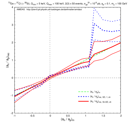
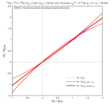
Figure 6: The reconstructed $a_{\rm n}/a_{\rm p}$ ratios estimated by Eqs. (39) (dashed blue) and (71) (solid red) and the lower and upper bounds of their 1$\sigma$ statistical uncertainties estimated by Eqs. (44) and (74) as functions of the input $a_{\rm n}/a_{\rm p}$ ratio. Besides ${}^{73}{\rm Ge}$ and ${}^{37}{\rm Cl}$, ${}^{28}{\rm Si}$ has been chosen as the third target for estimating $c_{{\rm p},(X,Y)}$ by Eqs. (72a) and (72b). For the SI cross section the nuclear form factor given in Eq. (18) has been used. The SI WIMP–proton cross section has been set as $10^{-8}$ pb (left) and $10^{-10}$ pb (right), respectively, whereas the SD WIMP–proton coupling $a_{\rm p}$ has been set as 0.1. The other parameters are as in Figs. 4. Note here that the scales of the $(a_{\rm n}/a_{\rm p})_{\rm rec}$–axes in two frames are different. See the text for further details.

In Figs. 6 I show the reconstructed $a_{\rm n}/a_{\rm p}$ ratios estimated by Eqs. (39) (dashed blue) and (71) (solid red) and the lower and upper bounds of their 1$\sigma$ statistical uncertainties estimated by Eqs. (44) and (74) as functions of the input $a_{\rm n}/a_{\rm p}$ ratio. For the SI cross section the nuclear form factor given in Eq. (18) has been used. The SI WIMP–proton cross section has been set as $10^{-8}$ pb (left) and $10^{-10}$ pb (right), respectively, whereas the SD WIMP–proton coupling $a_{\rm p}$ has been set as 0.1. Besides ${}^{73}{\rm Ge}$ and ${}^{37}{\rm Cl}$, ${}^{28}{\rm Si}$ has been chosen as the third target for estimating $c_{{\rm p},(X,Y)}$ by Eqs. (72a) and (72b).

In the left frame, it can be seen obviously that $a_{\rm n}/a_{\rm p}$ estimated by Eq. (39) (dashed blue) under the assumption of a dominant SD WIMP–nucleus interaction has two discontinuities around $(a_{\rm n}/a_{\rm p})_{\rm in}=1.16$ and $-0.08$ and the reconstructed $a_{\rm n}/a_{\rm p}$ ratio is systematically over–/underestimated. In contrast, $a_{\rm n}/a_{\rm p}$ determined by Eq. (71) (solid red) shows a more smooth estimate, although the reconstructed ratio is a bit underestimated with a relatively larger statistical uncertainty for input $a_{\rm n}/a_{\rm p}$ ratios around 1.16. However, once we set the input SI WIMP–proton cross section two orders of magnitude lower and thus the SD WIMP–nucleus cross section really dominates (the right frame), the $a_{\rm n}/a_{\rm p}$ ratios estimated by two methods show a clear compatibility.

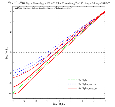
Figure 7: As in Figs. 6, except that ${}^{19}{\rm F}$, ${}^{127}{\rm I}$, and ${}^{28}{\rm Si}$ have been chosen as target nuclei. The scales used here are also different.

Figure 8: The reconstructed $a_{\rm n}/a_{\rm p}$ ratios estimated by Eqs. (39) (dashed blue) and (71) (solid red) and the lower and upper bounds of their 1$\sigma$ statistical uncertainties estimated by Eqs. (44) and (74) as functions of the input WIMP mass $m_{\chi}$. The input $a_{\rm n}/a_{\rm p}$ ratio has been set as 0.7, the other parameters are as in Figs. 6 and 7. Left: ${}^{73}{\rm Ge}$, ${}^{37}{\rm Cl}$, and ${}^{28}{\rm Si}$ have been chosen as the three target nuclei. Right: ${}^{19}{\rm F}$, ${}^{127}{\rm I}$, and ${}^{28}{\rm Si}$ have been chosen. Note here that the scales of the $(a_{\rm n}/a_{\rm p})_{\rm rec}$–axes in two frames are different.

In Figs. 7 the first two targets with both SI and SD sensitivities have been replaced again by ${}^{19}{\rm F}$ and ${}^{127}{\rm I}$. In contrast to Figs. 6, $a_{\rm n}/a_{\rm p}$ estimated by Eqs. (39) (dashed blue) and (71) (solid red) shown here are overestimated, especially the ratio reconstructed under the assumption of a dominant SD interaction. Nevertheless, the $a_{\rm n}/a_{\rm p}$ ratio estimated by Eqs. (71) (solid red) in both Figs. 6 and 7 show that the ratio between two SD WIMP–nucleos couplings could in principle be estimated correctly with an $\sim 20-40\%$ statistical uncertainty without prior information on the WIMP mass nor on the SI WIMP–nucleon cross section. The (in)compatibility between the reconstructed $a_{\rm n}/a_{\rm p}$ ratios under different assumptions and/or with different combinations of target nuclei could also allow us to check whether the SD WIMP–nucleus interaction really dominates or not.

Similar to the right frames of Figs. 4 and 5, Figs. 8 show the reconstructed $a_{\rm n}/a_{\rm p}$ ratios estimated by Eqs. (39) (dashed blue) and (71) (solid red) and the lower and upper bounds of their 1$\sigma$ statistical uncertainties estimated by Eqs. (44) and (74) as functions of the input WIMP mass $m_{\chi}$. The over–/underestimated $a_{\rm n}/a_{\rm p}$ ratios with different combinations of target nuclei can be seen obviously here. For input WIMP masses $m_{\chi}~{}\>\raisebox{-3.01385pt}{$\stackrel{{\scriptstyle\textstyle<}}{{\sim}}$}\>~{}50$ GeV, all estimates are as usual (strongly) underestimated. Nevertheless, for WIMP masses $m_{\chi}~{}\>\raisebox{-3.01385pt}{$\stackrel{{\scriptstyle\textstyle>}}{{\sim}}$}\>~{}50$ GeV, the reconstructed 1$\sigma$ statistical uncertainty intervals estimated by Eqs. (71) and (74) (solid red) could basically cover the input (true) value pretty well.

3.4 Choosing nuclei with ${\cal C}_{{\rm p},Y}=0$ and $\langle{\textstyle{S_{\rm p}}}\rangle_{X}\gg\langle{\textstyle{S_{\rm n}}}\rangle_{X}\simeq 0$

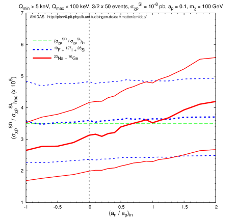
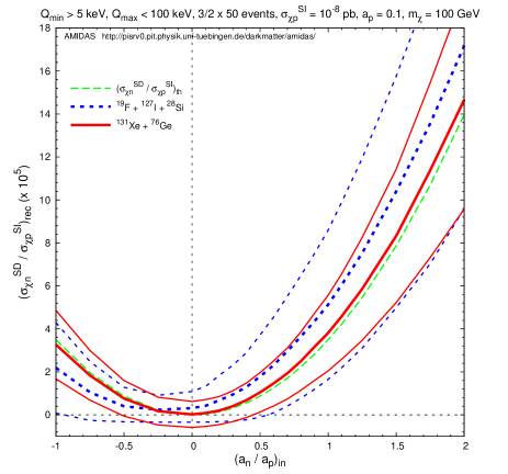
Figure 9: The reconstructed $\sigma_{\chi{\rm p}}^{\rm SD}/\sigma_{\chi{\rm p}}^{\rm SI}$ (left) and $\sigma_{\chi{\rm n}}^{\rm SD}/\sigma_{\chi{\rm p}}^{\rm SI}$ (right) and the lower and upper bounds of their 1$\sigma$ statistical uncertainties as functions of the input $a_{\rm n}/a_{\rm p}$, respectively. The dashed blue curves indicate the values estimated by Eq. (58) with $a_{\rm n}/a_{\rm p}$ estimated by Eq. (71) (not by Eq. (39)); whereas the solid red curves indicate the values estimated by Eq. (79). ${}^{76}{\rm Ge}$ has been chosen as the second target with only an SI sensitivity and combined with ${}^{23}{\rm Na}$ (for $\sigma_{\chi{\rm p}}^{\rm SD}/\sigma_{\chi{\rm p}}^{\rm SI}$) and ${}^{131}{\rm Xe}$ (for $\sigma_{\chi{\rm n}}^{\rm SD}/\sigma_{\chi{\rm p}}^{\rm SI}$) for using Eq. (79). Parameters are as in the left frame of Figs. 7, the input SI WIMP–proton cross section has been set as $10^{-8}$ pb. Note that, since we fix $\sigma_{\chi{\rm p}}^{\rm SI}$ and $a_{\rm p}$, the theoretical curve of $\sigma_{\chi{\rm p}}^{\rm SD}/\sigma_{\chi{\rm p}}^{\rm SI}$ is a constant, whereas the curve of $\sigma_{\chi{\rm n}}^{\rm SD}/\sigma_{\chi{\rm p}}^{\rm SI}\propto a_{\rm n}^{2}$ a parabola.

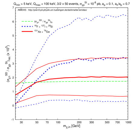
Figure 10: The reconstructed $\sigma_{\chi{\rm p}}^{\rm SD}/\sigma_{\chi{\rm p}}^{\rm SI}$ (left) and $\sigma_{\chi{\rm n}}^{\rm SD}/\sigma_{\chi{\rm p}}^{\rm SI}$ (right) and the lower and upper bounds of their 1$\sigma$ statistical uncertainties as functions of the input WIMP mass $m_{\chi}$, respectively. The input SI WIMP–proton cross section has been set as $10^{-8}$ pb and the input $a_{\rm n}/a_{\rm p}=0.7$, the other parameters and notations are as in Figs. 9.

In the expression (58) for the ratio of two WIMP–proton cross sections, there are four sources contributing statistical uncertainties, i.e., ${\cal C}_{{\rm p},(X,Y)}$ and ${\cal R}_{m,(X,Y)}$. In order to reduce the statistical uncertainty on the estimate of $\sigma_{\chi{\rm p}}^{\rm SD}/\sigma_{\chi{\rm p}}^{\rm SI}$, one can choose at first a nucleus with only an SI sensitivity as the second target:

$$\langle{\textstyle{S_{\rm p}}}\rangle_{Y}=\langle{\textstyle{S_{\rm n}}}\rangle_{Y}=0~{}\!,$$ (77)

i.e.,

$${\cal C}_{{\rm p},Y}=0~{}\!.$$ (78)

The expression in Eq. (58) can thus be reduced to [33]

$$\frac{\sigma_{\chi{\rm p}}^{\rm SD}}{\sigma_{\chi{\rm p}}^{\rm SI}}=\frac{F_{{\rm SI},Y}^{2}(Q_{{\rm min},Y})({\cal R}_{m,X}/{\cal R}_{m,Y})-F_{{\rm SI},X}^{2}(Q_{{\rm min},X})}{{\cal C}_{{\rm p},X}F_{{\rm SD},X}^{2}(Q_{{\rm min},X})}~{}\!.$$ (79)

Then we choose a nucleus with a (much) larger proton group spin as the first target:

$$\langle{\textstyle{S_{\rm p}}}\rangle_{X}\gg\langle{\textstyle{S_{\rm n}}}\rangle_{X}\simeq 0~{}\!,$$ (80)

in order to eliminate the $a_{\rm n}/a_{\rm p}$ dependence of ${\cal C}_{{\rm p},X}$ given in Eq. (51):

$${\cal C}_{{\rm p},X}\simeq\frac{4}{3}\Bigg{(}\frac{J_{X}+1}{J_{X}}\Bigg{)}\left[\frac{\langle{\textstyle{S_{\rm p}}}\rangle_{X}}{A_{X}}\right]^{2}~{}\!,$$ (82)

and the statistical uncertainty given in Eq. (75) can be reduced to

$$\sigma\left(\frac{\sigma_{\chi{\rm p}}^{\rm SD}}{\sigma_{\chi{\rm p}}^{\rm SI}}\right)\simeq\frac{F_{{\rm SI},Y}^{2}(Q_{{\rm min},Y})({\cal R}_{m,X}/{\cal R}_{m,Y})}{{\cal C}_{{\rm p},X}F_{{\rm SD},X}^{2}(Q_{{\rm min},X})}\left[\frac{\sigma^{2}(r_{X}(Q_{{\rm min},X}))}{r_{X}^{2}(Q_{{\rm min},X})}+\frac{\sigma^{2}(r_{Y}(Q_{{\rm min},Y}))}{r_{Y}^{2}(Q_{{\rm min},Y})}\right]^{1/2}~{}\!.$$ (83)

In Figs. 9 I show the reconstructed $\sigma_{\chi{\rm p}}^{\rm SD}/\sigma_{\chi{\rm p}}^{\rm SI}$ (left) and $\sigma_{\chi{\rm n}}^{\rm SD}/\sigma_{\chi{\rm p}}^{\rm SI}$ (right) as functions of the input $a_{\rm n}/a_{\rm p}$, respectively. The dashed blue curves indicate the values estimated by Eq. (58) with $a_{\rm n}/a_{\rm p}$ estimated by Eq. (71) (not by Eq. (39)); whereas the solid red curves indicate the values estimated by Eq. (79). Since, as shown in the left frame of Figs. 7, $a_{\rm n}/a_{\rm p}$ can be estimated pretty well by Eq. (71) with the target combination F and I in the range of interest $-1\leq|a_{\rm n}/a_{\rm p}|\leq 2$, $\sigma_{\chi{\rm p}}^{\rm SD}/\sigma_{\chi{\rm p}}^{\rm SI}$ shown in the left frame here can be reconstructed with an $\sim$ 40% statistical uncertainty by using the combination of ${}^{19}{\rm F}$ + ${}^{127}{\rm I}$ + ${}^{28}{\rm Si}$. On the other hand, the right frames of Figs. 9 and 10 show also that $\sigma_{\chi{\rm n}}^{\rm SD}/\sigma_{\chi{\rm p}}^{\rm SI}$ could still be estimated well with ${}^{131}{\rm Xe}$ and ${}^{76}{\rm Ge}$ by Eq. (79), although the statistical uncertainty is now larger ($\sim$ 70%).

4 Estimating ratios of the SI WIMP–nucleon couplings

So far I have used the theoretical prediction (7) that the SI scalar WIMP coupling on protons is approximately equal to the coupling on neutrons. For the sake of completeness, I consider in this section briefly the case that WIMPs have different SI scalar or vector couplings on protons and on neutrons [40]. For WIMPs having only the scalar interaction with nuclei, the expression (6) for $\sigma_{0}^{\rm SI}$ can be rewritten as

$$\sigma_{0}^{\rm SI}=\left(\frac{4}{\pi}\right)m_{\rm r,N}^{2}A^{2}\left[\left(\frac{Z}{A}\right)f_{\rm p}+\left(1-\frac{Z}{A}\right)f_{\rm n}\right]^{2}~{}\!.$$ (84)

Thus one can obtain the following replacements:

$$\frac{J+1}{J}\longrightarrow A^{2}~{}\!,$$ (85)

and

$$\langle{\textstyle{S_{\rm p}}}\rangle\longrightarrow\frac{Z}{A}~{}\!,~{}~{}~{}~{}~{}~{}~{}~{}~{}~{}~{}~{}~{}~{}~{}~{}\langle{\textstyle{S_{\rm n}}}\rangle\longrightarrow 1-\frac{Z}{A}~{}\!.$$ (86)

Substituting Eq. (85) into Eq. (41), we can get

$${\cal R}_{J,n,X}^{\rm SI}=\frac{1}{A_{X}}\sqrt{\frac{{\cal R}_{\sigma,X}}{{\cal R}_{n,X}}}~{}\!,$$ (87)

where ${\cal R}_{\sigma,X}$ and ${\cal R}_{n,X}$ are given in Eqs. (38) and (42). Then the ratio between the scalar WIMP coupling on protons and on neutrons can be estimated analogously to Eq. (39) as

$$\left(\frac{f_{\rm n}}{f_{\rm p}}\right)_{\pm,n}=-\frac{Z_{X}\pm Z_{Y}\sqrt{{\cal R}_{\sigma,X}/{\cal R}_{n,X}}\sqrt{{\cal R}_{n,Y}/{\cal R}_{\sigma,Y}}}{(A_{X}-Z_{X})\pm(A_{Y}-Z_{Y})\sqrt{{\cal R}_{\sigma,X}/{\cal R}_{n,X}}\sqrt{{\cal R}_{n,Y}/{\cal R}_{\sigma,Y}}}~{}\!,$$ (88)

with the following statistical uncertainty:

$$\sigma\left(\left(\frac{f_{\rm n}}{f_{\rm p}}\right)_{\pm,n}\right) = \frac{\Big{|}A_{X}Z_{Y}-A_{Y}Z_{X}\Big{|}\sqrt{{\cal R}_{\sigma,X}/{\cal R}_{n,X}}\sqrt{{\cal R}_{n,Y}/{\cal R}_{\sigma,Y}}}{2\bigg{[}(A_{X}-Z_{X})\pm(A_{Y}-Z_{Y})\sqrt{{\cal R}_{\sigma,X}/{\cal R}_{n,X}}\sqrt{{\cal R}_{n,Y}/{\cal R}_{\sigma,Y}}\bigg{]}^{2}}$$ (89)

$$~{}~{}\times\Bigg{\{}\sum_{i,j=1}^{3}\left[\frac{1}{{\cal R}_{n,X}}\left(\frac{\partial{\cal R}_{n,X}}{\partial c_{i,X}}\right)-\frac{1}{{\cal R}_{\sigma,X}}\left(\frac{\partial{\cal R}_{\sigma,X}}{\partial c_{i,X}}\right)\right]\Bigg{.}$$

$$~{}~{}~{}~{}~{}~{}~{}~{}~{}~{}~{}~{}~{}~{}~{}~{}\times\left[\frac{1}{{\cal R}_{n,X}}\left(\frac{\partial{\cal R}_{n,X}}{\partial c_{j,X}}\right)-\frac{1}{{\cal R}_{\sigma,X}}\left(\frac{\partial{\cal R}_{\sigma,X}}{\partial c_{j,X}}\right)\right]{\rm cov}(c_{i,X},c_{j,X})$$

$$~{}~{}~{}~{}~{}~{}~{}~{}~{}~{}~{}~{}\Bigg{.}+(X\longrightarrow Y)\Bigg{\}}^{1/2}~{}\!.$$

Note that, firstly, since $A-Z>0$ for all nuclei, the inner solution of $f_{\rm n}/f_{\rm p}$ given in Eq. (88) with a much smaller statistical uncertainty is always the “$+$” solution. Secondly, the two coincident points of the “$+$” and “$-$” soulutions decided by $-Z_{X}/(A_{X}-Z_{X})$ and $-Z_{Y}/(A_{Y}-Z_{Y})$ are however always negative. While, for lighter nuclei, e.g. ${}^{28}{\rm Si}$ and ${}^{19}{\rm F}$, the values of $-Z/(A-Z)$ are $\sim-1$; for heavier nuclei, e.g. ${}^{127}{\rm I}$ or ${}^{131}{\rm Xe}$, these values are $\sim-0.7$. This means that, unfortunately, for confirming the $f_{\rm n}/f_{\rm p}$ ratio with the theoretical predicted value of $\sim 1$, we can only use the “outer ($-$)” solutions given in Eq. (88) with much larger statistical uncertainties and data sets with piles of events should therefore be required.

On the other hand, assuming that WIMPs have only the vector interaction with nuclei, according to the expression (5) for $\sigma_{0}^{\rm vector}$, we can write down the expression for the relative strength of two “vector” couplings directly as

$$\left(\frac{b_{\rm n}}{b_{\rm p}}\right)_{\pm,n}=-\frac{2Z_{X}\pm 2Z_{Y}\sqrt{{\cal R}_{\sigma,X}/{\cal R}_{n,X}}\sqrt{{\cal R}_{n,Y}/{\cal R}_{\sigma,Y}}}{(A_{X}-Z_{X})\pm(A_{Y}-Z_{Y})\sqrt{{\cal R}_{\sigma,X}/{\cal R}_{n,X}}\sqrt{{\cal R}_{n,Y}/{\cal R}_{\sigma,Y}}}~{}\!.$$ (90)

with the following statistical uncertainty:

$$\sigma\left(\left(\frac{b_{\rm n}}{b_{\rm p}}\right)_{\pm,n}\right) = \frac{\Big{|}A_{X}Z_{Y}-A_{Y}Z_{X}\Big{|}\sqrt{{\cal R}_{\sigma,X}/{\cal R}_{n,X}}\sqrt{{\cal R}_{n,Y}/{\cal R}_{\sigma,Y}}}{\left[(A_{X}-Z_{X})\pm(A_{Y}-Z_{Y})\sqrt{{\cal R}_{\sigma,X}/{\cal R}_{n,X}}\sqrt{{\cal R}_{n,Y}/{\cal R}_{\sigma,Y}}\right]^{2}}$$ (91)

$$~{}~{}\times\Bigg{\{}\sum_{i,j=1}^{3}\left[\frac{1}{{\cal R}_{n,X}}\left(\frac{\partial{\cal R}_{n,X}}{\partial c_{i,X}}\right)-\frac{1}{{\cal R}_{\sigma,X}}\left(\frac{\partial{\cal R}_{\sigma,X}}{\partial c_{i,X}}\right)\right]\Bigg{.}$$

$$~{}~{}~{}~{}~{}~{}~{}~{}~{}~{}~{}~{}~{}~{}~{}~{}\times\left[\frac{1}{{\cal R}_{n,X}}\left(\frac{\partial{\cal R}_{n,X}}{\partial c_{j,X}}\right)-\frac{1}{{\cal R}_{\sigma,X}}\left(\frac{\partial{\cal R}_{\sigma,X}}{\partial c_{j,X}}\right)\right]{\rm cov}(c_{i,X},c_{j,X})$$

$$~{}~{}~{}~{}~{}~{}~{}~{}~{}~{}~{}~{}\Bigg{.}+(X\longrightarrow Y)\Bigg{\}}^{1/2}~{}\!.$$

Note that the factor “2” appearing in the denominator of the prefacor in Eq. (89) has been cancelled here.

5 Summary and conclusions

In this paper, I presented methods for determining ratios between different WIMP–nucleon couplings/cross sections from elastic WIMP–nucleus scattering experiments. All methods presented here are independent of the model of halo WIMPs as well as (practically) of the as yet unknown WIMP mass. Assuming that an exponential–like shape of the recoil spectrum is confirmed from experimental data, the required information are only the measured recoil energies and the number of events in the first energy bin from at least two direct detection experiments with different detector materials having spin sensitivities contributed from protons and/or from neutrons. Even better, our simulations show that, for estimating the relative strengths of different WIMP–nucleon couplings, one would only need events in the lowest available energy ranges.

In order to avoid the uncertainty on the local WIMP density $\rho_{0}$, our analyses are based on combining two (or more) experiments using different target nuclei. By assuming, as the first step, that the SD WIMP–nucleus interaction dominates over the SI one, the expression for determining the ratio between two SD WIMP–nucleon couplings, $a_{\rm n}/a_{\rm p}$, has been rederived [33]. Then our simulations with different combinations of target nuclei show that, in order to obtain an unambiguous result with much smaller statistical uncertainty in the range of interest: $|a_{\rm n}/a_{\rm p}|~{}\>\raisebox{-3.01385pt}{$\stackrel{{\scriptstyle\textstyle<}}{{\sim}}$}\>~{}2$, nuclei with sensitivities on both protons and neutrons should be more suitable than nuclei being sensitive (almost) only on protons or on neutrons.

More generally, I considered also the combination of the SI and SD WIMP–nucleus cross sections. By using three different targets, two of them have non–zero group spins from protons and/or from neutrons, the second expression for determining the ratio between two SD WIMP–nucleon couplings can be rederived [33]. Although its statistical uncertainty depends on the relative strength between the SD and SI WIMP–nucleus interactions, the (in)compatibility between the $a_{\rm n}/a_{\rm p}$ ratio reconstructed under different assumptions and/or with different combinations of target nuclei could allow us to check whether the SD WIMP–nucleus interaction really dominates. Moreover, by using two or three different nuclei, one or two of them have non–zero group spins from protons and/or from neutrons, one can in principle also determine the ratios of the WIMP–proton/neutron cross sections to the SI ones, $\sigma_{\chi{\rm p}}^{\rm SD}/\sigma_{\chi{\rm p}}^{\rm SI}$ and $\sigma_{\chi{\rm n}}^{\rm SD}/\sigma_{\chi{\rm p}}^{\rm SI}$, directly.

Our simulations presented here are based on several simplified assumptions. Firstly, the sample to be analyzed contains only signal events, i.e., is free of background^, . Secondly, all experimental systematic uncertainties as well as the uncertainty on the measurement of the recoil energy have been ignored. The energy resolution of most currently running and projected detectors is so good that its uncertainty can be neglected compared to the statistical uncertainty with (very) few events in the foreseeable future.

In summary, I demonstrated in this paper the use of our new methods for extracting information on WIMP–nucleon couplings/cross sections, which are independent of models of WIMPs from particle physics as well as of models of the Galactic halo from cosmology. By combining with information on the estimation of the SI WIMP–nucleon coupling [44, 34], one could in principle estimate the absolute values of the spin–dependent couplings/cross sections. These information could help us not only to give constraints on different models of particle physics in the parameter space, but also to understand the nature of halo Dark Matter particles as well as to distinguish them between candidates predicted in different scenarios [21, 22, 23, 5].

Acknowledgments

The author appreciates M. Drees and M. Kakizaki for useful discussions and detailed comments on the preliminary draft. The author would also like to thank the Physikalisches Institut der Universität Tübingen for the technical support of the computational work presented in this article. This work was partially supported by the National Science Council of R.O.C. under contract no. NSC-99-2811-M-006-031 and the LHC Physics Focus Group, National Center of Theoretical Sciences, R.O.C..

Appendix A Lists of needed formulae

Here I list all formulae needed for our model–independent data analyses described in this article. Detailed derivations and discussions can be found in Refs. [32, 31].

A.1 Estimating $r(Q_{\rm min})$ and $I_{n}(Q_{\rm min},Q_{\rm max})$

First, consider experimental data described by

$${\textstyle Q_{n}-\frac{b_{n}}{2}}\leq Q_{n,i}\leq{\textstyle Q_{n}+\frac{b_{n}}{2}}~{}\!,~{}~{}~{}~{}~{}~{}~{}~{}~{}~{}~{}~{}i=1,~{}2,~{}\cdots,~{}N_{n},~{}n=1,~{}2,~{}\cdots,~{}B.$$ (A1)

Here the total energy range between $Q_{\rm min}$ and $Q_{\rm max}$ has been divided into $B$ bins with central points $Q_{n}$ and widths $b_{n}$. In each bin, $N_{n}$ events will be recorded. Since the recoil spectrum $dR/dQ$ is expected to be approximately exponential, the following ansatz for the measured recoil spectrum (before normalized by the experimental exposure ${\cal E}$) in the $n$th bin has been introduced [32]:

$$\left(\frac{dR}{dQ}\right)_{{\rm expt},~{}\!n}\equiv\left(\frac{dR}{dQ}\right)_{{\rm expt},~{}\!Q\simeq Q_{n}}\equiv r_{n}~{}\!e^{k_{n}(Q-Q_{s,n})}~{}\!.$$ (A2)

Here $r_{n}$ is the standard estimator for $(dR/dQ)_{\rm expt}$ at $Q=Q_{n}$:

$$r_{n}=\frac{N_{n}}{b_{n}}~{}\!,$$ (A3)

$k_{n}$ is the logarithmic slope of the recoil spectrum in the $n$th $Q-$bin, which can be computed numerically from the average value of the measured recoil energies in this bin:

$$\overline{Q-Q_{n}}|_{n}=\left(\frac{b_{n}}{2}\right)\coth\left(\frac{k_{n}b_{n}}{2}\right)-\frac{1}{k_{n}}~{}\!,$$ (A4)

where

$$\overline{(Q-Q_{n})^{\lambda}}|_{n}\equiv\frac{1}{N_{n}}\sum_{i=1}^{N_{n}}\left(Q_{n,i}-Q_{n}\right)^{\lambda}~{}\!.$$ (A5)

The error on the logarithmic slope $k_{n}$ can be estimated from Eq. (A4) directly as

$$\sigma^{2}(k_{n})=k_{n}^{4}\left\{1-\left[\frac{k_{n}b_{n}/2}{\sinh(k_{n}b_{n}/2)}\right]^{2}\right\}^{-2}\sigma^{2}\left(\overline{Q-Q_{n}}|_{n}\right)~{}\!,$$ (A6)

with

$$\sigma^{2}\left(\overline{Q-Q_{n}}|_{n}\right)=\frac{1}{N_{n}-1}\bigg{[}\overline{(Q-Q_{n})^{2}}|_{n}-\overline{Q-Q_{n}}|_{n}^{2}\bigg{]}~{}\!.$$ (A7)

$Q_{s,n}$ in the ansatz (A2) is the shifted point at which the leading systematic error due to the ansatz is minimal [32],

$$Q_{s,n}=Q_{n}+\frac{1}{k_{n}}\ln\left[\frac{\sinh(k_{n}b_{n}/2)}{k_{n}b_{n}/2}\right]~{}\!.$$ (A8)

Note that $Q_{s,n}$ differs from the central point of the $n$th bin, $Q_{n}$. From the ansatz (A2), the counting rate at $Q=Q_{\rm min}$ can be calculated by

$$r(Q_{\rm min})=r_{1}e^{k_{1}(Q_{\rm min}-Q_{s,1})}~{}\!,$$ (A9)

and its statistical error can be expressed as

$$\sigma^{2}(r(Q_{\rm min}))=r^{2}(Q_{\rm min})\left\{\frac{1}{N_{1}}+\left[\frac{1}{k_{1}}-\left(\frac{b_{1}}{2}\right)\left(1+\coth\left(\frac{b_{1}k_{1}}{2}\right)\right)\right]^{2}\sigma^{2}(k_{1})\right\}~{}\!,$$ (A10)

since

$$\sigma^{2}(r_{n})=\frac{N_{n}}{b_{n}^{2}}~{}\!.$$ (A11)

Finally, since all $I_{n}$ are determined from the same data, they are correlated with

$${\rm cov}(I_{n},I_{m})=\sum_{a=1}^{N_{\rm tot}}\frac{Q_{a}^{(n+m-2)/2}}{F^{4}(Q_{a})}~{}\!,$$ (A12)

where the sum runs over all events with recoil energy between $Q_{\rm min}$ and $Q_{\rm max}$. And the correlation between the errors on $r(Q_{\rm min})$, which is calculated entirely from the events in the first bin, and on $I_{n}$ is given by

$${\rm cov}(r(Q_{\rm min}),I_{n})$$ (A13)

$$= r(Q_{\rm min})~{}\!I_{n}(Q_{\rm min},Q_{\rm min}+b_{1})$$

$$~{}~{}~{}~{}\times\left\{\frac{1}{N_{1}}+\left[\frac{1}{k_{1}}-\left(\frac{b_{1}}{2}\right)\left(1+\coth\left(\frac{b_{1}k_{1}}{2}\right)\right)\right]\right.$$

$$~{}~{}~{}~{}~{}~{}~{}~{}~{}~{}~{}~{}~{}~{}\times\left.\left[\frac{I_{n+2}(Q_{\rm min},Q_{\rm min}+b_{1})}{I_{n}(Q_{\rm min},Q_{\rm min}+b_{1})}-Q_{1}+\frac{1}{k_{1}}-\left(\frac{b_{1}}{2}\right)\coth\left(\frac{b_{1}k_{1}}{2}\right)\right]\sigma^{2}(k_{1})\right\}~{}\!;$$

note that the sums $I_{i}$ here only count in the first bin, which ends at $Q=Q_{\rm min}+b_{1}$.

On the other hand, with a functional form of the recoil spectrum (e.g., fitted to experimental data), $(dR/dQ)_{\rm expt}$, one can use the following integral forms to replace the summations given above. Firstly, the average $Q-$value in the $n$th bin defined in Eq. (A5) can be calculated by

$$\overline{(Q-Q_{n})^{\lambda}}|_{n}=\frac{1}{N_{n}}\int_{Q_{n}-b_{n}/2}^{Q_{n}+b_{n}/2}\left(Q-Q_{n}\right)^{\lambda}\left(\frac{dR}{dQ}\right)_{\rm expt}dQ~{}\!.$$ (A14)

For $I_{n}(Q_{\rm min},Q_{\rm max})$ given in Eq. (35), we have

$$I_{n}(Q_{\rm min},Q_{\rm max})=\int_{Q_{\rm min}}^{Q_{\rm max}}\frac{Q^{(n-1)/2}}{F^{2}(Q)}\left(\frac{dR}{dQ}\right)_{\rm expt}dQ~{}\!,$$ (A15)

and similarly for the covariance matrix for $I_{n}$ in Eq. (A12),

$${\rm cov}(I_{n},I_{m})=\int_{Q_{\rm min}}^{Q_{\rm max}}\frac{Q^{(n+m-2)/2}}{F^{4}(Q)}\left(\frac{dR}{dQ}\right)_{\rm expt}dQ~{}\!.$$ (A16)

Remind that $(dR/dQ)_{\rm expt}$ is the measured recoil spectrum before normalized by the exposure. Finally, $I_{i}(Q_{\rm min},Q_{\rm min}+b_{1})$ needed in Eq. (A13) can be calculated by

$$I_{n}(Q_{\rm min},Q_{\rm min}+b_{1})=\int_{Q_{\rm min}}^{Q_{\rm min}+b_{1}}\frac{Q^{(n-1)/2}}{F^{2}(Q)}\bigg{[}r_{1}~{}\!e^{k_{1}(Q-Q_{s,1})}\bigg{]}dQ~{}\!.$$ (A17)

Note that, firstly, $r(Q_{\rm min})$ and $I_{n}(Q_{\rm min},Q_{\rm min}+b_{1})$ should be estimated by Eqs. (A9) and (A17) with $r_{1}$, $k_{1}$ and $Q_{s,1}$ estimated by Eqs. (A3), (A4), and (A8) in order to use the other formulae for estimating the (correlations between the) statistical errors without any modification. Secondly, $r(Q_{\rm min})$ and $I_{n}(Q_{\rm min},Q_{\rm max})$ estimated from a scattering spectrum fitted to experimental data are usually not model–independent any more. Moreover, for the use of Eqs. (35), (A12), (A15), (A16), and (A17) the elastic nuclear form factor $F^{2}(Q)$ should be understood to be chosen for the SI and SD WIMP–nucleon cross section correspondingly.

A.2 Derivatives of ${\cal R}_{n,X}$ and ${\cal R}_{\sigma,X}$

First, from Eq. (42) one can find explicit expressions for the derivatives of ${\cal R}_{n,X}$ with respect to $c_{i,X}$ are:

$$\frac{\partial{\cal R}_{n,X}}{\partial I_{n,X}}=\frac{n+1}{n}\left[\frac{F_{X}^{2}(Q_{{\rm min},X})}{2Q_{{\rm min},X}^{(n+1)/2}r_{X}(Q_{{\rm min},X})+(n+1)I_{n,X}F_{X}^{2}(Q_{{\rm min},X})}\right]{\cal R}_{n,X}~{}\!,$$ (A18a)

$$\frac{\partial{\cal R}_{n,X}}{\partial I_{0,X}}=-\frac{1}{n}\left[\frac{F_{X}^{2}(Q_{{\rm min},X})}{2Q_{{\rm min},X}^{1/2}r_{X}(Q_{{\rm min},X})+I_{0,X}F_{X}^{2}(Q_{{\rm min},X})}\right]{\cal R}_{n,X}~{}\!,$$ (A18b)

and

$$\frac{\partial{\cal R}_{n,X}}{\partial r_{X}(Q_{{\rm min},X})} = \frac{2}{n}\left[\frac{Q_{{\rm min},X}^{(n+1)/2}I_{0,X}-(n+1)Q_{{\rm min},X}^{1/2}I_{n,X}}{2Q_{{\rm min},X}^{(n+1)/2}r_{X}(Q_{{\rm min},X})+(n+1)I_{n,X}F_{X}^{2}(Q_{{\rm min},X})}\right]$$ (A18c)

$$~{}~{}~{}~{}~{}~{}~{}~{}~{}~{}~{}~{}~{}~{}~{}~{}\times\left[\frac{F_{X}^{2}(Q_{{\rm min},X})}{2Q_{{\rm min},X}^{1/2}r_{X}(Q_{{\rm min},X})+I_{0,X}F_{X}^{2}(Q_{{\rm min},X})}\right]{\cal R}_{n,X}~{}\!;$$

explicit expressions for the derivatives of ${\cal R}_{n,Y}$ with respect to $c_{i,Y}$ can be given analogously. Note that, firstly, factors ${\cal R}_{n,(X,Y)}$ appear in all these expressions, which can practically be cancelled by the prefactors in the bracket in Eq. (44). Secondly, all the $I_{0,(X,Y)}$ and $I_{n,(X,Y)}$ should be understood to be computed according to Eq. (35) or (A15) with integration limits $Q_{\rm min}$ and $Q_{\rm max}$ specific for that target.

Similarly, expressions for the derivatives of ${\cal R}_{\sigma,X}$ can be computed from Eq. (38) as

$$\frac{\partial{\cal R}_{\sigma,X}}{\partial I_{0,X}}=\left[\frac{F_{X}^{2}(Q_{{\rm min},X})}{2Q_{{\rm min},X}^{1/2}r_{X}(Q_{{\rm min},X})+I_{0,X}F_{X}^{2}(Q_{{\rm min},X})}\right]{\cal R}_{\sigma,X}~{}\!,$$ (A19a)

$$\frac{\partial{\cal R}_{\sigma,X}}{\partial r_{X}(Q_{{\rm min},X})}=\left[\frac{2Q_{{\rm min},X}^{1/2}}{2Q_{{\rm min},X}^{1/2}r_{X}(Q_{{\rm min},X})+I_{0,X}F_{X}^{2}(Q_{{\rm min},X})}\right]{\cal R}_{\sigma,X}~{}\!;$$ (A19b)

and similarly for the derivatives of ${\cal R}_{\sigma,Y}$. Remind that factors ${\cal R}_{\sigma,(X,Y)}$ appearing here can also be cancelled by the prefactors in the bracket in Eq. (44).

A.3 Derivatives of $\sigma_{\chi{\rm p}}^{\rm SD}/\sigma_{\chi{\rm p}}^{\rm SI}$

From the expression (58) for estimating $\sigma_{\chi{\rm p}}^{\rm SD}/\sigma_{\chi{\rm p}}^{\rm SI}$, its derivatives with respect to ${\cal C}_{{\rm p},(X,Y)}$ can be given as

$$\frac{\partial}{\partial{\cal C}_{{\rm p},X}}\left(\frac{\sigma_{\chi{\rm p}}^{\rm SD}}{\sigma_{\chi{\rm p}}^{\rm SI}}\right)=-\frac{F_{{\rm SD},X}^{2}(Q_{{\rm min},X}){\cal R}_{m,Y}}{{\cal C}_{{\rm p},X}F_{{\rm SD},X}^{2}(Q_{{\rm min},X}){\cal R}_{m,Y}-{\cal C}_{{\rm p},Y}F_{{\rm SD},Y}^{2}(Q_{{\rm min},Y}){\cal R}_{m,X}}\left(\frac{\sigma_{\chi{\rm p}}^{\rm SD}}{\sigma_{\chi{\rm p}}^{\rm SI}}\right)~{}\!,$$ (A20a)

and

$$\frac{\partial}{\partial{\cal C}_{{\rm p},Y}}\left(\frac{\sigma_{\chi{\rm p}}^{\rm SD}}{\sigma_{\chi{\rm p}}^{\rm SI}}\right)=\frac{F_{{\rm SD},Y}^{2}(Q_{{\rm min},Y}){\cal R}_{m,X}}{{\cal C}_{{\rm p},X}F_{{\rm SD},X}^{2}(Q_{{\rm min},X}){\cal R}_{m,Y}-{\cal C}_{{\rm p},Y}F_{{\rm SD},Y}^{2}(Q_{{\rm min},Y}){\cal R}_{m,X}}\left(\frac{\sigma_{\chi{\rm p}}^{\rm SD}}{\sigma_{\chi{\rm p}}^{\rm SI}}\right)~{}\!.$$ (A20b)

Meanwhile, the derivatives of $\sigma_{\chi{\rm p}}^{\rm SD}/\sigma_{\chi{\rm p}}^{\rm SI}$ with respect to ${\cal R}_{m,(X,Y)}$ are

$$\frac{\partial}{\partial{\cal R}_{m,X}}\left(\frac{\sigma_{\chi{\rm p}}^{\rm SD}}{\sigma_{\chi{\rm p}}^{\rm SI}}\right)$$ (A21a)

$$= -\frac{\Big{[}{\cal C}_{{\rm p},X}F_{{\rm SD},X}^{2}(Q_{{\rm min},X})F_{{\rm SI},Y}^{2}(Q_{{\rm min},Y})-{\cal C}_{{\rm p},Y}F_{{\rm SD},Y}^{2}(Q_{{\rm min},Y})F_{{\rm SI},X}^{2}(Q_{{\rm min},X})\Big{]}{\cal R}_{m,Y}}{\Big{[}{\cal C}_{{\rm p},X}F_{{\rm SD},X}^{2}(Q_{{\rm min},X}){\cal R}_{m,Y}-{\cal C}_{{\rm p},Y}F_{{\rm SD},Y}^{2}(Q_{{\rm min},Y}){\cal R}_{m,X}\Big{]}^{2}}~{}\!,$$

and

$$\frac{\partial}{\partial{\cal R}_{m,Y}}\left(\frac{\sigma_{\chi{\rm p}}^{\rm SD}}{\sigma_{\chi{\rm p}}^{\rm SI}}\right)$$ (A21b)

$$= \frac{\Big{[}{\cal C}_{{\rm p},Y}F_{{\rm SD},Y}^{2}(Q_{{\rm min},Y})F_{{\rm SI},X}^{2}(Q_{{\rm min},X})-{\cal C}_{{\rm p},X}F_{{\rm SD},X}^{2}(Q_{{\rm min},X})F_{{\rm SI},Y}^{2}(Q_{{\rm min},Y})\Big{]}{\cal R}_{m,X}}{\Big{[}{\cal C}_{{\rm p},X}F_{{\rm SD},X}^{2}(Q_{{\rm min},X}){\cal R}_{m,Y}-{\cal C}_{{\rm p},Y}F_{{\rm SD},Y}^{2}(Q_{{\rm min},Y}){\cal R}_{m,X}\Big{]}^{2}}~{}\!.$$

On the other hand, from expression (51) for ${\cal C}_{\rm p}$ one can find that

$$\frac{\partial{\cal C}_{\rm p}}{\partial(a_{\rm n}/a_{\rm p})}=\frac{2{\cal C}_{\rm p}}{\langle{\textstyle{S_{\rm p}}}\rangle/\langle{\textstyle{S_{\rm n}}}\rangle+a_{\rm n}/a_{\rm p}}~{}\!,$$ (A22)

and, since we estimate in fact always $a_{\rm n}/a_{\rm p}$, one needs practically

$$\frac{\partial{\cal C}_{\rm n}}{\partial(a_{\rm n}/a_{\rm p})}=-\frac{2{\cal C}_{\rm n}}{a_{\rm n}/a_{\rm p}+(\langle{\textstyle{S_{\rm n}}}\rangle/\langle{\textstyle{S_{\rm p}}}\rangle)(a_{\rm n}/a_{\rm p})^{2}}~{}\!.$$ (A23)

A.4 Derivatives of $(a_{\rm n}/a_{\rm p})_{\pm}^{\rm SI+SD}$

At first, from the first and second lines of the expression (71), we have,

$$\frac{\partial}{\partial c_{{\rm p},X}}\left(\frac{a_{\rm n}}{a_{\rm p}}\right)_{\pm}^{\rm SI+SD} = -\frac{1}{\left(c_{{\rm p},X}s_{{\rm n/p},X}^{2}-c_{{\rm p},Y}s_{{\rm n/p},Y}^{2}\right)^{2}}$$ (A30a)

$$~{}~{}~{}~{}~{}~{}\times\Bigg{[}c_{{\rm p},Y}s_{{\rm n/p},X}s_{{\rm n/p},Y}\left(s_{{\rm n/p},X}-s_{{\rm n/p},Y}\right)\Bigg{.}$$

$$~{}~{}~{}~{}~{}~{}~{}~{}~{}~{}~{}~{}~{}~{}~{}~{}\Bigg{.}\pm\frac{1}{2}\sqrt{\frac{c_{{\rm p},Y}}{c_{{\rm p},X}}}\left(c_{{\rm p},X}s_{{\rm n/p},X}^{2}+c_{{\rm p},Y}s_{{\rm n/p},Y}^{2}\right)\left|s_{{\rm n/p},X}-s_{{\rm n/p},Y}\right|\Bigg{]}$$

$$= \left\{\begin{array}[]{l l l}\\ \displaystyle\mp\frac{\sqrt{c_{{\rm p},X}c_{{\rm p},Y}}\left(s_{{\rm n/p},X}-s_{{\rm n/p},Y}\right)}{2c_{{\rm p},X}\left(\sqrt{c_{{\rm p},X}}s_{{\rm n/p},X}\mp\sqrt{c_{{\rm p},Y}}s_{{\rm n/p},Y}\right)^{2}}~{}\!,&{}{}&({\rm for}~{}s_{{\rm n/p},X}>s_{{\rm n/p},Y}),\\ {}\\ {}\\ \displaystyle\pm\frac{\sqrt{c_{{\rm p},X}c_{{\rm p},Y}}\left(s_{{\rm n/p},X}-s_{{\rm n/p},Y}\right)}{2c_{{\rm p},X}\left(\sqrt{c_{{\rm p},X}}s_{{\rm n/p},X}\pm\sqrt{c_{{\rm p},Y}}s_{{\rm n/p},Y}\right)^{2}}~{}\!,&&({\rm for}~{}s_{{\rm n/p},X}<s_{{\rm n/p},Y}),\\ {}\\ \end{array}\right.$$

and

$$\frac{\partial}{\partial c_{{\rm p},Y}}\left(\frac{a_{\rm n}}{a_{\rm p}}\right)_{\pm}^{\rm SI+SD} = \frac{1}{\left(c_{{\rm p},X}s_{{\rm n/p},X}^{2}-c_{{\rm p},Y}s_{{\rm n/p},Y}^{2}\right)^{2}}$$ (A36b)

$$~{}~{}~{}~{}~{}~{}\times\Bigg{[}c_{{\rm p},X}s_{{\rm n/p},X}s_{{\rm n/p},Y}\left(s_{{\rm n/p},X}-s_{{\rm n/p},Y}\right)\Bigg{.}$$

$$~{}~{}~{}~{}~{}~{}~{}~{}~{}~{}~{}~{}~{}~{}~{}~{}\Bigg{.}\pm\frac{1}{2}\sqrt{\frac{c_{{\rm p},X}}{c_{{\rm p},Y}}}\left(c_{{\rm p},X}s_{{\rm n/p},X}^{2}+c_{{\rm p},Y}s_{{\rm n/p},Y}^{2}\right)\left|s_{{\rm n/p},X}-s_{{\rm n/p},Y}\right|\Bigg{]}$$

$$= \left\{\begin{array}[]{l l l}\\ \displaystyle\pm\frac{\sqrt{c_{{\rm p},X}c_{{\rm p},Y}}\left(s_{{\rm n/p},X}-s_{{\rm n/p},Y}\right)}{2c_{{\rm p},Y}\left(\sqrt{c_{{\rm p},X}}s_{{\rm n/p},X}\mp\sqrt{c_{{\rm p},Y}}s_{{\rm n/p},Y}\right)^{2}}~{}\!,&{}{}&({\rm for}~{}s_{{\rm n/p},X}>s_{{\rm n/p},Y}),\\ {}\\ {}\\ \displaystyle\mp\frac{\sqrt{c_{{\rm p},X}c_{{\rm p},Y}}\left(s_{{\rm n/p},X}-s_{{\rm n/p},Y}\right)}{2c_{{\rm p},Y}\left(\sqrt{c_{{\rm p},X}}s_{{\rm n/p},X}\pm\sqrt{c_{{\rm p},Y}}s_{{\rm n/p},Y}\right)^{2}}~{}\!,&&({\rm for}~{}s_{{\rm n/p},X}<s_{{\rm n/p},Y}).\\ {}\\ \end{array}\right.$$

Then, from the definition (72a) of $c_{{\rm p},X}$, one can get directly

$$\frac{\partial c_{{\rm p},X}}{\partial r_{X}(Q_{{\rm min},X})}=0~{}\!,$$ (A37a)

$$\frac{\partial c_{{\rm p},X}}{\partial r_{Y}(Q_{{\rm min},Y})}=F_{{\rm SI},Z}^{2}(Q_{{\rm min},Z})F_{{\rm SD},X}^{2}(Q_{{\rm min},X})\cdot\frac{4}{3}\Bigg{(}\frac{J_{X}+1}{J_{X}}\Bigg{)}\left[\frac{\langle{\textstyle{S_{\rm p}}}\rangle_{X}}{A_{X}}\right]^{2}\cdot\frac{{\cal R}_{m,YZ}}{r_{Y}(Q_{{\rm min},Y})}~{}\!,$$ (A37b)

and

$$\frac{\partial c_{{\rm p},X}}{\partial r_{Z}(Q_{{\rm min},Z})}=-F_{{\rm SI},Z}^{2}(Q_{{\rm min},Z})F_{{\rm SD},X}^{2}(Q_{{\rm min},X})\cdot\frac{4}{3}\Bigg{(}\frac{J_{X}+1}{J_{X}}\Bigg{)}\left[\frac{\langle{\textstyle{S_{\rm p}}}\rangle_{X}}{A_{X}}\right]^{2}\cdot\frac{{\cal R}_{m,YZ}}{r_{Z}(Q_{{\rm min},Z})}~{}\!.$$ (A37c)

Similarly, from the definition (72b) of $c_{{\rm p},Y}$, we have

$$\frac{\partial c_{{\rm p},Y}}{\partial r_{X}(Q_{{\rm min},X})}=F_{{\rm SI},Z}^{2}(Q_{{\rm min},Z})F_{{\rm SD},Y}^{2}(Q_{{\rm min},Y})\cdot\frac{4}{3}\Bigg{(}\frac{J_{Y}+1}{J_{Y}}\Bigg{)}\left[\frac{\langle{\textstyle{S_{\rm p}}}\rangle_{Y}}{A_{Y}}\right]^{2}\cdot\frac{{\cal R}_{m,XZ}}{r_{X}(Q_{{\rm min},X})}~{}\!,$$ (A38a)

$$\frac{\partial c_{{\rm p},Y}}{\partial r_{Y}(Q_{{\rm min},Y})}=0~{}\!,$$ (A38b)

and

$$\frac{\partial c_{{\rm p},Y}}{\partial r_{Z}(Q_{{\rm min},Z})}=-F_{{\rm SI},Z}^{2}(Q_{{\rm min},Z})F_{{\rm SD},Y}^{2}(Q_{{\rm min},Y})\cdot\frac{4}{3}\Bigg{(}\frac{J_{Y}+1}{J_{Y}}\Bigg{)}\left[\frac{\langle{\textstyle{S_{\rm p}}}\rangle_{Y}}{A_{Y}}\right]^{2}\cdot\frac{{\cal R}_{m,XZ}}{r_{Z}(Q_{{\rm min},Z})}~{}\!.$$ (A38c)

References

- [1] G. Jungman, M. Kamionkowski and K. Griest, “Supersymmetric Dark Matter”, Phys. Rep. 267, 195 (1996), arXiv:hep-ph/9506380.
- [2] G. Bertone, D. Hooper and J. Silk, “Particle Dark Matter: Evidence, Candidates and Constraints”, Phys. Rep. 405, 279 (2005), arXiv:hep-ph/0404175.
- [3] P. F. Smith and J. D. Lewin, “Dark Matter Detection”, Phys. Rep. 187, 203 (1990).
- [4] J. D. Lewin and P. F. Smith, “Review of Mathematics, Numerical Factors, and Corrections for Dark Matter Experiments Based on Elastic Nuclear Recoil”, Astropart. Phys. 6, 87 (1996).
- [5] R. C. Cotta, J. S. Gainer, J. L. Hewett and T. G. Rizzo, “Dark Matter in the MSSM”, New J. Phys. 11, 105026 (2009), arXiv:0903.4409 [hep-ph].
- [6] D. R. Tovey et al., “A New Model–Independent Method for Extracting Spin–Dependent Cross Section Limits from Dark Matter Searches”, Phys. Lett. B 488, 17 (2000), arXiv:hep-ph/0005041.
- [7] F. Giuliani and T. A. Girard, “Model–Independent Limits from Spin–Dependent WIMP Dark Matter Experiments”, Phys. Rev. D 71, 123503 (2005), arXiv:hep-ph/0502232.
- [8] T. A. Girard and F. Giuliani, “On the Direct Search for Spin–Dependent WIMP Interactions”, Phys. Rev. D 75, 043512 (2007), arXiv:hep-ex/0511044.
- [9] Enriched , V. A. Bednyakov, H. V. Klapdor-Kleingrothaus and I. V. Krivosheina, “New Constraints on Spin–Dependent WIMP–Neutron Interactions from HDMS with Natural Ge and Ge-73”, Phys. Atom. Nucl. 71, 111 (2008).
- [10] F. Giuliani, “Model–Independent Assessment of Current Direct Searches for Spin-Dependent Dark Matter”, Phys. Rev. Lett. 93, 161301 (2004), arXiv:hep-ph/0404010.
- [11] UK Dark Matter Collab., G. J. Alner et al., “Limits on WIMP Cross–Sections from the NAIAD Experiment at the Boulby Underground Laboratory”, Phys. Lett. B 616, 17 (2005), arXiv:hep-ex/0504031.
- [12] KIMS Collab., H. S. Lee et al., “Limits on WIMP–Nucleon Cross Section with CsI(Tl) Crystal Detectors”, Phys. Rev. Lett. 99, 091301 (2007), arXiv:0704.0423 [astro-ph].
- [13] SIMPLE Collab., M. Felizardo et al., “First Results of the Phase II SIMPLE Dark Matter Search”, Phys. Rev. Lett. 105, 211301 (2010), arXiv:1003.2987 [astro-ph.CO].
- [14] M.-C. Piro, for the PICASSO Collab., “Status of the PICASSO Experiment for Spin–Dependent Dark Matter Searches”, arXiv:1005.5455 [astro-ph.IM] (2010).
- [15] COUPP Collab., E. Behnke et al., “Improved Limits on Spin–Dependent WIMP–Proton Interactions from a Two Liter CF3I Bubble Chamber”, Phys. Rev. Lett. 106, 021303 (2011), arXiv:1008.3518 [astro-ph.CO].
- [16] CDMS Collab., D. S. Akerib et al., “Limits on Spin–Dependent WIMP–Nucleon Interactions from the Cryogenic Dark Matter Search”, Phys. Rev. D 73, 011102 (2006), arXiv:astro-ph/0509269.
- [17] XENON10 Collab., J. Angle et al., “Limits on Spin–Dependent WIMP–Nucleon Cross–Sections from the XENON10 Experiment”, Phys. Rev. Lett. 101, 091301 (2008), arXiv:0805.2939 [astro-ph].
- [18] ZEPLIN-III Collab., V. N. Lebedenko et al., “Limits on the Spin–Dependent WIMP–Nucleon Cross–Sections from the First Science Run of the ZEPLIN-III Experiment”, Phys. Rev. Lett. 103, 151302 (2009), arXiv:0901.4348 [hep-ex].
- [19] V. A. Bednyakov, “Aspects of Spin Dependent Dark Matter Search”, Phys. Atom. Nucl. 67, 1931 (2004), arXiv:hep-ph/0310041.
- [20] J. Ellis, K. A. Olive and C. Savage, “Hadronic Uncertainties in the Elastic Scattering of Supersymmetric Dark Matter”, Phys. Rev. D 77, 065026 (2008), arXiv:0801.3656 [hep-ph].
- [21] G. Bertone, D. G. Cerdeo, J. I. Collar and B. C. Odom, “WIMP Identification Through a Combined Measurement of Axial and Scalar Couplings”, Phys. Rev. Lett. 99, 151301 (2007), arXiv:0705.2502 [astro-ph].
- [22] V. Barger, W. Y. Keung and G. Shaughnessy, “Spin Dependence of Dark Matter Scattering”, Phys. Rev. D 78, 056007 (2008), arXiv:0806.1962 [hep-ph].
- [23] G. Bélanger, E. Nezri and A. Pukhov, “Discriminating Dark Matter Candidates Using Direct Detection”, Phys. Rev. D 79, 015008 (2009), arXiv:0810.1362 [hep-ph].
- [24] S. P. Ahlen et al., “Limits on Cold Dark Matter Candidates from an Ultralow Background Germanium Spectrometer”, Phys. Lett. B 195, 603 (1987).
- [25] K. Freese, J. Frieman and A. Gould, “Signal Modulation in Cold Dark Matter Detection”, Phys. Rev. D 37, 3388 (1988).
- [26] J. Engel, “Nuclear Form–Factors for the Scattering of Weakly Interacting Massive Particles”, Phys. Lett. B 264, 114 (1991).
- [27] R. H. Helm, “Inelastic and Elastic Scattering of 187-Mev Electrons from Selected Even–Even Nuclei”, Phys. Rev. 104, 1466 (1956).
- [28] G. Eder, “Nuclear Forces”, MIT Press, Chapter 7 (1968).
- [29] H. V. Klapdor-Kleingrothaus, I. V. Krivosheina and C. Tomei, “New Limits on Spin–Dependent Weakly Interacting Massive Particle (WIMP) Nucleon Coupling”, Phys. Lett. B 609, 226 (2005).
- [30] C.-L. Shan and M. Drees, “Determining the WIMP Mass from Direct Dark Matter Detection Data”, arXiv:0710.4296 [hep-ph] (2007).
- [31] M. Drees and C.-L. Shan, “Model–Independent Determination of the WIMP Mass from Direct Dark Matter Detection Data”, J. Cosmol. Astropart. Phys. 0806, 012 (2008), arXiv:0803.4477 [hep-ph].
- [32] M. Drees and C.-L. Shan, “Reconstructing the Velocity Distribution of Weakly Interacting Massive Particles from Direct Dark Matter Detection Data”, J. Cosmol. Astropart. Phys. 0706, 011 (2007), arXiv:astro-ph/0703651.
- [33] C.-L. Shan, “Extracting Dark Matter Properties Model–Independently from Direct Detection Experiments”, Mod. Phys. Lett. A 25, 951 (2010), arXiv:1003.0962 [hep-ph].
- [34] C.-L. Shan, “Estimating the Spin–Independent WIMP–Nucleon Coupling from Direct Dark Matter Detection Data”, arXiv:1103.0481 [hep-ph] (2011).
- [35] C.-L. Shan, “Effects of Residue Background Events in Direct Dark Matter Detection Experiments on the Determinations of Ratios of WIMP–Nucleon Cross Sections”, arXiv:1104.5305 [hep-ph] (2011).
- [36] XENON Collab., J. Angle et al., “First Results from the XENON10 Dark Matter Experiment at the Gran Sasso National Laboratory”, Phys. Rev. Lett. 100, 021303 (2008), arXiv:0706.0039 [astro-ph].
- [37] CDMS Collab., Z. Ahmed et al., “Results from the Final Exposure of the CDMS II Experiment”, Science 327, 1619 (2010), arXiv:0912.3592 [astro-ph.CO].
- [38] XENON100 Collab., E. Aprile et al., “First Dark Matter Results from the XENON100 Experiment”, Phys. Rev. Lett. 105, 131302 (2010), arXiv:1005.0380 [astro-ph.CO].
- [39] V. Kozlov, for the EDELWEISS Collab., “Latest Results of the Direct Dark Matter Search with the EDELWEISS-2 Experiment”, J. Phys. Conf. Ser. 259, 012037 (2010), arXiv:1010.5947 [astro-ph.IM].
- [40] J. L. Feng, J. Kumar, D. Marfatia and D. Sanford, “Isospin–Violating Dark Matter”, arXiv:1102.4331 [hep-ph] (2011).
- [41] E. Aprile and L. Baudis, for the XENON100 Collab., “Status and Sensitivity Projections for the XENON100 Dark Matter Experiment”, PoS IDM2008, 018 (2008), arXiv:0902.4253 [astro-ph.IM].
- [42] CRESST Collab., R. F. Lang et al., “Discrimination of Recoil Backgrounds in Scintillating Calorimeters”, Astropart. Phys. 33, 60 (2010), arXiv:0903.4687 [astro-ph.IM]; CRESST Collab., R. F. Lang et al., “Electron and Gamma Background in CRESST Detectors”, Astropart. Phys. 32, 318 (2010), arXiv:0905.4282 [astro-ph.IM]; CRESST Collab., J. Schmaler et al., “Status of the CRESST Dark Matter Search”, AIP Conf. Proc. 1185, 631 (2009), arXiv:0912.3689 [astro-ph.IM].
- [43] EDELWEISS Collab., A. Broniatowski et al., “A New High–Background–Rejection Dark Matter Ge Cryogenic Detector”, Phys. Lett. B 681, 305 (2009), arXiv:0905.0753 [astro-ph.IM]; EDELWEISS Collab., E. Armengaud et al., “First Results of the EDELWEISS-II WIMP Search Using Ge Cryogenic Detectors with Interleaved Electrodes”, Phys. Lett. B 687, 294 (2010), arXiv:0912.0805 [astro-ph.CO].
- [44] M. Drees and C.-L. Shan, “Constraining the Spin–Independent WIMP–Nucleon Coupling from Direct Dark Matter Detection Data”, PoS IDM2008, 110 (2008), arXiv:0809.2441 [hep-ph].