Quantum learning algorithms for quantum measurements

Abstract

We study quantum learning algorithms for quantum measurements. The optimal learning algorithm is derived for arbitrary von Neumann measurements in the case of training with one or two examples. The analysis of the case of three examples reveals that, differently from the learning of unitary gates, the optimal algorithm for learning of quantum measurements cannot be parallelized, and requires quantum memories for the storage of information.

I Introduction

The rapid development of an information technology in the last decades made the optimization of information processing tasks an important field of computer science. For example one needs to optimize database search, as well as tasks that emerged due to internet e.g. algorithms for anti-spam filters and internet search engines. The last two tasks are instances of the so called machine learning vapnik , which can be defined as follows. Suppose we have a black box evaluating an unknown function $f$ and we have access to $N$ uses of it. However, after we lose the access to the black box we need to evaluate $f$ on an input that was not previously available. Naturally any machine learning has two phases – training and retrieving. The knowledge on $f$ acquired in the training phase of the strategy is encoded into a bit string that is later used as a program governing the retrieval phase. Obviously, if $N$ is greater or equal to the number of possible inputs of $f$ then the training part of the strategy can acquire complete knowledge of $f$. The same task, termed quantum learning, can be generalized to quantum theory. In this case the black box performs an unknown quantum transformation $\mathcal{T}$. The result of the training phase is a quantum state $\psi_{\mathcal{T}}$. This state has to be kept in the quantum memory until the retrieving phase, where it enters together with the unknown state $\rho$ into the retrieving channel that mimics the action of $\mathcal{T}$ on $\rho$. We can immediately observe substantial difference to machine learning. Even for finite dimensional quantum systems there does not exist a finite $N$ for which the quantum learning works perfectly. Indeed, even if the training part of the strategy would encode full information about $\mathcal{T}$ into the finite dimensional state $\psi_{\mathcal{T}}$, the no programming theorem of Nielsen nielsen prevents us to retrieve the transformation perfectly.

A closely related problem to quantum learning was studied as a quantum version of pattern recognition algorithms sasa ; sasacarl . For the case of quantum learning of channels, the first analysis was published in Ref. molmer , where very simple processing techniques were studied for learning of particular gates like the Grover oracle Grover or the discrete Fourier transform. Learning of unitary black boxes was analyzed in Ref. learnunit . Surprisingly, it turns out that the task of quantum learning of unitaries can be fully parallelized, which means that the optimal training phase is achieved by applying the $N$ uses of the black box on the fixed entangled state. Another surprising feature of the aforementioned training phase is that it is an optimal estimation procedure and hence the quantum memory can be replaced by a classical storage of the estimated unitary black box. The simulation then consists in the conditional application of the gate corresponding to the estimated parameters.

In the present paper we will consider the case in which the black box to be learnt is a device performing a Von Neumann measurement, namely a projective non-degenerate Positive Operator Valued Measure (POVM) $\mathbf{E}:=\{E_{i}\}$. We will show that for measuring black boxes the surprising features of optimal learning of unitary black boxes disappear. In particular, we will show that the optimal algorithm cannot be parallelized, leading to a training phase that lasts an increasing time versus the number of examples. Moreover, the optimal training does not consist of optimal estimation, thus requiring a coherent quantum memory for the storage of the learnt measurement.

The paper is organized as follows. In Sec II we review some notation and preliminary concepts used in the analysis. In Sec. III we expose the mathematical formulation of the general problem of optimal learning in mathematical terms. In Sec. IV the problem is simplified exploiting all the symmetries that can be useful. The problem is then solved in Sec. V for the cases $N=1$, $N=2$ and $N=3$. Finally, the paper is closed by concluding remarks in Sec. VI.

II Preliminary concepts

In this section we review some notions of the theory of quantum networks comblong ; architecture ; memoryeff . The main feature of this approach is the representation of quantum networks in terms of suitably normalized positive operators.

The nodes of a quantum network $\mathcal{R}$ are elementary boxes linked by wires. Elementary boxes represent state preparations, channels, quantum operations, or effects. The most general pictorial representation of a quantum network is a directed acyclic graph, where the vertices represent elementary boxes and the arrows represent the quantum systems traveling within the network in the direction induced by the input-output relation.

By stretching the connections in the graph we can give the quantum network the shape of a comb, i.e. any quantum network $\mathcal{R}$ is equivalent to a sequence of $N$ quantum operations $\{T_{i}\}_{i=1}^{N}$ with some unconnected input and output subsystems, as follows

(1)

If all the $N$ quantum operations are trace preserving (i.e. they are quantum channels) $\mathcal{R}$ is a deterministic quantum network, otherwise $\mathcal{R}$ is a probabilistic quantum network. The ordering of the teeth is induced by the causal order defined by the flow of quantum information inside the quantum network. Referring to the scheme in Eq. (1) we label each wire with an integer number $j$: accordingly, the Hilbert space of the system represented by wire $j$ is denoted as $\mathscr{H}_{j}$.

Since a quantum network $\mathcal{R}$ is a concatenation of quantum operations it can be considered as a quantum operation itself $\mathcal{R}:\mathcal{L}(\mathscr{H}_{even})\to\mathcal{L}(\mathscr{H}_{odd})$ where we defined $\mathscr{H}_{even}=\bigotimes_{i=0}^{N}\mathscr{H}_{2i}$ and $\mathscr{H}_{odd}=\bigotimes_{i=0}^{N}\mathscr{H}_{2i+1}$. That being so, it is possible to define the Choi-Jamiołkowsky operator of a quantum network as

$$R:=\mathcal{R}\otimes\mathcal{I}(|\omega\rangle\langle\omega|)$$ (2)

$$R\in\mathcal{L}(\mathscr{H}_{even}\otimes\mathscr{H}_{odd}),\qquad R\leq 0$$

where $\mathcal{I}$ is the identity map and $\left|{\omega}\right\rangle\in\mathscr{H}_{even}^{\otimes 2}$, $\left|{\omega}\right\rangle=\sum_{n}\left|{n}\right\rangle\left|{n}\right\rangle$ ($\{\left|{n}\right\rangle\}$ is an orthonormal basis of $\mathscr{H}_{even}$). The Choi-Jamiołkowsky operator of a quantum network is called quantum comb of the network. If $\mathcal{R}$ is a deterministic quantum network it is possible to prove that its Choi-Jamiołkowsky operator $R$ must satisfy the recursive normalization constraint

$${\rm Tr}_{2k-1}[R^{(k)}]=I_{2k-2}\otimes R^{(k-1)}\qquad k=1,\dots,N~{}$$ (3)

where $R^{(N)}=R$, $R^{(0)}=1$, $R^{(k)}\in\mathcal{L}(\mathscr{H}_{{odd}_{k}}\otimes\mathscr{H}_{{even}_{k}})$ with $\mathscr{H}_{{even}_{k}}=\bigotimes_{j=0}^{k-1}\mathscr{H}_{2j}$ and $\mathscr{H}_{{odd}_{k}}=\bigotimes_{j=0}^{k-1}\mathscr{H}_{2j+1}$, is the comb of the reduced circuit $\mathcal{R}^{(k)}$ obtained by discarding the last $N-k$ teeth. It is relevant to stress that each positive operator that satisfies Eq. (3) corresponds to a valid deterministic quantum network. This gives us a correspondence between the set of positive operators satisfying Eq. (3) and the set of deterministic quantum networks.

On the other hand, the Choi-Jamiołkowsky operator of a probabilistic quantum network $\mathcal{R}$, must satisfy

$$0\leq R\leq S$$ (4)

where $S$ is a Choi-Jamiołkowsky operator of a deterministic quantum network. An important theorem proves comblong that any positive operator, upon suitable rescaling, represents a probabilistic quantum network.

Two quantum networks $\mathcal{R}_{1}$ and $\mathcal{R}_{2}$ can be connected by linking input wires of one network with output wires of the other network thus forming the network $\mathcal{R}_{1}*\mathcal{R}_{2}$. The Choi-Jamiołkowsky operator of the composite network $\mathcal{R}_{1}*\mathcal{R}_{2}$ is the link product of the operators $R_{1}$ and $R_{2}$ which is defined as follows:

$$R_{1}*R_{2}={\rm Tr}_{\mathcal{K}}[R_{1}R_{2}^{\theta_{\mathcal{K}}}]$$ (5)

where $\theta_{\mathcal{K}}$ denotes the partial transposition (with respect to a fixed orthonormal basis) over the Hilbert space $\mathcal{K}$ of the connected wires and ${\rm Tr}_{\mathcal{K}}$ denotes the partial trace over $\mathcal{K}$.

II.1 Generalized Instrument

The aim of this paper is to study quantum networks that replicate quantum measurements. A generalized quantum instrument is set of probabilistic quantum networks $\boldsymbol{\mathcal{R}}:=\{\mathcal{R}_{i}\}$ such that the set $\mathbf{R}=\{R_{i}\}$ of the Choi-Jamiołkowsky operators of its components satisfies the following condition:

$$\sum_{i}R_{i}:=R_{\Omega}$$ (6)

where $R_{\Omega}$ corresponds to a deterministic quantum network. Every probabilistic quantum network belongs to some generalized quantum instrument, and viceversa every generalized quantum instrument represents some set of probabilistic quantum networks.

III the optimization problem

The learning scenario can be formulated as a quantum network that accepts $N$ measurements into the open slots and works as a POVM on the remaining system. Here is a diagram representing the $N=2$ scenario,

$$\begin{aligned} \lx@xy@svg{\hbox{\raise 0.0pt\hbox{\kern 9.16656pt\hbox{\ignorespaces\ignorespaces\ignorespaces\hbox{\vtop{\kern 0.0pt\offinterlineskip\halign{\entry@#!@&&\entry@@#!@\cr&&&&&&&&\\&&&&&&&&\\&&&&&&&&\\}}}\ignorespaces{\hbox{\kern 0.0pt\raise 0.0pt\hbox{\hbox{\kern-3.0pt\raise 0.0pt\hbox{\hbox{\kern 3.0pt\raise 0.0pt\hbox{$\textstyle{}$}}}}}}}{\hbox{\kern 16.16653pt\raise 0.0pt\hbox{\hbox{\kern-3.0pt\raise 0.0pt\hbox{\hbox{\kern 3.0pt\raise 0.0pt\hbox{$\textstyle{}$}}}}}}}{\hbox{\kern 32.02762pt\raise 0.0pt\hbox{\hbox{\kern-3.0pt\raise 0.0pt\hbox{\hbox{\kern 3.0pt\raise 0.0pt\hbox{$\textstyle{}$}}}}}}}{\hbox{\kern 47.8887pt\raise 0.0pt\hbox{\hbox{\kern-3.0pt\raise 0.0pt\hbox{\hbox{\kern 3.0pt\raise 0.0pt\hbox{$\textstyle{}$}}}}}}}{\hbox{\kern 64.05524pt\raise 0.0pt\hbox{\hbox{\kern-3.0pt\raise 0.0pt\hbox{\hbox{\kern 3.0pt\raise 0.0pt\hbox{$\textstyle{}$}}}}}}}{\hbox{\kern 80.22177pt\raise 0.0pt\hbox{\hbox{\kern-3.0pt\raise 0.0pt\hbox{\hbox{\kern 3.0pt\raise 0.0pt\hbox{$\textstyle{}$}}}}}}}{\hbox{\kern 96.08286pt\raise 0.0pt\hbox{\hbox{\kern-3.0pt\raise 0.0pt\hbox{\hbox{\kern 3.0pt\raise 0.0pt\hbox{$\textstyle{}$}}}}}}}{\hbox{\kern 111.94394pt\raise 0.0pt\hbox{\hbox{\kern-2.5pt\raise 5.0pt\hbox{$\textstyle{4}$}}}}}{\hbox{\kern 118.94391pt\raise 0.0pt\hbox{\hbox{\kern 5.0pt\raise 0.0pt\hbox{$\textstyle{\hphantom{\;\;\;}}$}}}}}\ignorespaces\ignorespaces\ignorespaces\ignorespaces{}{\hbox{\lx@xy@droprule}}\ignorespaces{}{\hbox{\lx@xy@droprule}}{\hbox{\lx@xy@droprule}}{\hbox{\kern-9.16656pt\raise-23.8333pt\hbox{\hbox{\kern 5.0pt\raise 0.0pt\hbox{$\textstyle{\hphantom{\;\;\;}}$}}}}}\ignorespaces\ignorespaces\ignorespaces\ignorespaces{\hbox{\kern-4.16656pt\raise-35.74994pt\hbox{\hbox{\kern 0.0pt\raise 0.0pt\hbox{$\textstyle{\;\;\;}$}}}}}\ignorespaces\ignorespaces\ignorespaces\ignorespaces\ignorespaces\ignorespaces{\hbox{\lx@xy@droprule}}\ignorespaces\ignorespaces\ignorespaces\ignorespaces\ignorespaces{\hbox{\lx@xy@droprule}}\ignorespaces\ignorespaces\ignorespaces\ignorespaces\ignorespaces\ignorespaces{\hbox{\lx@xy@droprule}}\ignorespaces\ignorespaces\ignorespaces\ignorespaces\ignorespaces\ignorespaces\ignorespaces{\hbox{\lx@xy@droprule}}\ignorespaces{\hbox{\kern-9.16656pt\raise-19.33333pt\hbox{\hbox{\kern 0.0pt\raise-8.99994pt\hbox{$\textstyle{\hbox{\cirbuild@}}$}}}}}\ignorespaces{\hbox{\kern-9.16656pt\raise-52.16656pt\hbox{\hbox{\kern 0.0pt\raise 8.99994pt\hbox{$\textstyle{\hbox{\cirbuild@}}$}}}}}{\hbox{\kern 16.16653pt\raise-23.8333pt\hbox{\hbox{\kern-2.5pt\raise 5.0pt\hbox{$\textstyle{0}$}}}}}\ignorespaces\ignorespaces\ignorespaces\ignorespaces{}{\hbox{\lx@xy@droprule}}\ignorespaces{}{\hbox{\lx@xy@droprule}}{\hbox{\lx@xy@droprule}}{\hbox{\kern 23.1665pt\raise-23.8333pt\hbox{\hbox{\kern 0.0pt\raise 0.0pt\hbox{$\textstyle{\lx@xy@svgnested{\hbox{\raise 0.0pt\hbox{\kern 11.80557pt\hbox{{\hbox{\kern-5.91666pt\raise 0.0pt\hbox{\hbox{\kern 2.51387pt\raise-3.41666pt\hbox{$\textstyle{\vphantom{\rule{0.0pt}{1.00006pt}\mathbf{E}}}$}}}}}{\hbox{\kern-5.91666pt\raise 0.0pt\hbox{\hbox{\kern 0.0pt\raise 0.0pt\hbox{\cirbuild@}}}}}\ignorespaces{\hbox{\kern-6.80557pt\raise 0.0pt\hbox{\hbox{\kern 0.0pt\raise-3.41666pt\hbox{$\textstyle{\mathbf{E}}$}}}}}\ignorespaces\ignorespaces\ignorespaces\ignorespaces\ignorespaces{\hbox{\kern-11.80557pt\raise 5.91666pt\hbox{\hbox{\kern 0.0pt\raise-3.41666pt\hbox{$\textstyle{\hphantom{\mathbf{E}}}$}}}}}\ignorespaces\ignorespaces\ignorespaces{\hbox{\lx@xy@droprule}}\ignorespaces\ignorespaces\ignorespaces\ignorespaces\ignorespaces{\hbox{\kern-11.80557pt\raise-5.91666pt\hbox{\hbox{\kern 0.0pt\raise-3.41666pt\hbox{$\textstyle{\hphantom{\mathbf{E}}}$}}}}}\ignorespaces\ignorespaces\ignorespaces{\hbox{\lx@xy@droprule}}\ignorespaces\ignorespaces\ignorespaces{\hbox{\kern-11.80557pt\raise 5.91666pt\hbox{\hbox{\kern 0.0pt\raise-3.41666pt\hbox{$\textstyle{\hphantom{\mathbf{E}}}$}}}}}\ignorespaces\ignorespaces\ignorespaces{\hbox{\kern-11.80557pt\raise-5.91666pt\hbox{\hbox{\kern 0.0pt\raise-3.41666pt\hbox{$\textstyle{\hphantom{\mathbf{E}}}$}}}}}\ignorespaces\ignorespaces\ignorespaces{\hbox{\lx@xy@droprule}}}}}}}$}}}}}\ignorespaces\ignorespaces\ignorespaces\ignorespaces{}{\hbox{\lx@xy@droprule}}\ignorespaces{}{\hbox{\lx@xy@droprule}}{\hbox{\lx@xy@droprule}}{\hbox{\kern 47.8887pt\raise-23.8333pt\hbox{\hbox{\kern-2.5pt\raise 5.0pt\hbox{$\textstyle{1}$}}}}}\ignorespaces\ignorespaces\ignorespaces\ignorespaces{}{\hbox{\hbox{\kern 0.0pt\raise-1.0pt\hbox{\lx@xy@droprule}}\hbox{\kern 0.0pt\raise 1.0pt\hbox{\lx@xy@droprule}}}}\ignorespaces{}{\hbox{\hbox{\kern 0.0pt\raise-1.0pt\hbox{\lx@xy@droprule}}\hbox{\kern 0.0pt\raise 1.0pt\hbox{\lx@xy@droprule}}}}{\hbox{\hbox{\kern 0.0pt\raise-1.0pt\hbox{\lx@xy@droprule}}\hbox{\kern 0.0pt\raise 1.0pt\hbox{\lx@xy@droprule}}}}{\hbox{\kern 54.88867pt\raise-23.8333pt\hbox{\hbox{\kern 5.0pt\raise 0.0pt\hbox{$\textstyle{\hphantom{\;\;\;}}$}}}}}\ignorespaces\ignorespaces\ignorespaces\ignorespaces{}{\hbox{\hbox{\kern 0.0pt\raise-1.0pt\hbox{\lx@xy@droprule}}\hbox{\kern 0.0pt\raise 1.0pt\hbox{\lx@xy@droprule}}}}\ignorespaces{}{\hbox{\hbox{\kern 0.0pt\raise-1.0pt\hbox{\lx@xy@droprule}}\hbox{\kern 0.0pt\raise 1.0pt\hbox{\lx@xy@droprule}}}}{\hbox{\hbox{\kern 0.0pt\raise-1.0pt\hbox{\lx@xy@droprule}}\hbox{\kern 0.0pt\raise 1.0pt\hbox{\lx@xy@droprule}}}}{\hbox{\kern 80.22177pt\raise-23.8333pt\hbox{\hbox{\kern-2.5pt\raise 5.0pt\hbox{$\textstyle{2}$}}}}}\ignorespaces\ignorespaces\ignorespaces\ignorespaces{}{\hbox{\lx@xy@droprule}}\ignorespaces{}{\hbox{\lx@xy@droprule}}{\hbox{\lx@xy@droprule}}{\hbox{\kern 87.22174pt\raise-23.8333pt\hbox{\hbox{\kern 0.0pt\raise 0.0pt\hbox{$\textstyle{\lx@xy@svgnested{\hbox{\raise 0.0pt\hbox{\kern 11.80557pt\hbox{{\hbox{\kern-5.91666pt\raise 0.0pt\hbox{\hbox{\kern 2.51387pt\raise-3.41666pt\hbox{$\textstyle{\vphantom{\rule{0.0pt}{1.00006pt}\mathbf{E}}}$}}}}}{\hbox{\kern-5.91666pt\raise 0.0pt\hbox{\hbox{\kern 0.0pt\raise 0.0pt\hbox{\cirbuild@}}}}}\ignorespaces{\hbox{\kern-6.80557pt\raise 0.0pt\hbox{\hbox{\kern 0.0pt\raise-3.41666pt\hbox{$\textstyle{\mathbf{E}}$}}}}}\ignorespaces\ignorespaces\ignorespaces\ignorespaces\ignorespaces{\hbox{\kern-11.80557pt\raise 5.91666pt\hbox{\hbox{\kern 0.0pt\raise-3.41666pt\hbox{$\textstyle{\hphantom{\mathbf{E}}}$}}}}}\ignorespaces\ignorespaces\ignorespaces{\hbox{\lx@xy@droprule}}\ignorespaces\ignorespaces\ignorespaces\ignorespaces\ignorespaces{\hbox{\kern-11.80557pt\raise-5.91666pt\hbox{\hbox{\kern 0.0pt\raise-3.41666pt\hbox{$\textstyle{\hphantom{\mathbf{E}}}$}}}}}\ignorespaces\ignorespaces\ignorespaces{\hbox{\lx@xy@droprule}}\ignorespaces\ignorespaces\ignorespaces{\hbox{\kern-11.80557pt\raise 5.91666pt\hbox{\hbox{\kern 0.0pt\raise-3.41666pt\hbox{$\textstyle{\hphantom{\mathbf{E}}}$}}}}}\ignorespaces\ignorespaces\ignorespaces{\hbox{\kern-11.80557pt\raise-5.91666pt\hbox{\hbox{\kern 0.0pt\raise-3.41666pt\hbox{$\textstyle{\hphantom{\mathbf{E}}}$}}}}}\ignorespaces\ignorespaces\ignorespaces{\hbox{\lx@xy@droprule}}}}}}}$}}}}}\ignorespaces\ignorespaces\ignorespaces\ignorespaces{}{\hbox{\lx@xy@droprule}}\ignorespaces{}{\hbox{\lx@xy@droprule}}{\hbox{\lx@xy@droprule}}{\hbox{\kern 111.94394pt\raise-23.8333pt\hbox{\hbox{\kern-2.5pt\raise 5.0pt\hbox{$\textstyle{3}$}}}}}\ignorespaces\ignorespaces\ignorespaces\ignorespaces{}{\hbox{\hbox{\kern 0.0pt\raise-1.0pt\hbox{\lx@xy@droprule}}\hbox{\kern 0.0pt\raise 1.0pt\hbox{\lx@xy@droprule}}}}\ignorespaces{}{\hbox{\hbox{\kern 0.0pt\raise-1.0pt\hbox{\lx@xy@droprule}}\hbox{\kern 0.0pt\raise 1.0pt\hbox{\lx@xy@droprule}}}}{\hbox{\hbox{\kern 0.0pt\raise-1.0pt\hbox{\lx@xy@droprule}}\hbox{\kern 0.0pt\raise 1.0pt\hbox{\lx@xy@droprule}}}}{\hbox{\kern 118.94391pt\raise-23.8333pt\hbox{\hbox{\kern 5.0pt\raise 0.0pt\hbox{$\textstyle{\hphantom{\;\;\;}}$}}}}}\ignorespaces\ignorespaces\ignorespaces\ignorespaces{}{\hbox{\hbox{\kern 0.0pt\raise-1.0pt\hbox{\lx@xy@droprule}}\hbox{\kern 0.0pt\raise 1.0pt\hbox{\lx@xy@droprule}}}}\ignorespaces{}{\hbox{\hbox{\kern 0.0pt\raise-1.0pt\hbox{\lx@xy@droprule}}\hbox{\kern 0.0pt\raise 1.0pt\hbox{\lx@xy@droprule}}}}{\hbox{\hbox{\kern 0.0pt\raise-1.0pt\hbox{\lx@xy@droprule}}\hbox{\kern 0.0pt\raise 1.0pt\hbox{\lx@xy@droprule}}}}{\hbox{\kern-9.16656pt\raise-47.6666pt\hbox{\hbox{\kern 5.0pt\raise 0.0pt\hbox{$\textstyle{\hphantom{\;\;\;}}$}}}}}{\hbox{\kern 16.16653pt\raise-47.6666pt\hbox{\hbox{\kern-3.0pt\raise 0.0pt\hbox{\hbox{\kern 3.0pt\raise 0.0pt\hbox{$\textstyle{\ignorespaces\ignorespaces\ignorespaces\ignorespaces}$}}}}}}}\ignorespaces\ignorespaces\ignorespaces\ignorespaces{}{\hbox{\lx@xy@droprule}}\ignorespaces{}{\hbox{\lx@xy@droprule}}{\hbox{\lx@xy@droprule}}{\hbox{\kern 32.02762pt\raise-47.6666pt\hbox{\hbox{\kern-3.0pt\raise 0.0pt\hbox{\hbox{\kern 3.0pt\raise 0.0pt\hbox{$\textstyle{\ignorespaces\ignorespaces\ignorespaces\ignorespaces}$}}}}}}}\ignorespaces\ignorespaces\ignorespaces\ignorespaces{}{\hbox{\lx@xy@droprule}}\ignorespaces{}{\hbox{\lx@xy@droprule}}{\hbox{\lx@xy@droprule}}{\hbox{\kern 47.8887pt\raise-47.6666pt\hbox{\hbox{\kern-3.0pt\raise 0.0pt\hbox{\hbox{\kern 3.0pt\raise 0.0pt\hbox{$\textstyle{\ignorespaces\ignorespaces\ignorespaces\ignorespaces}$}}}}}}}\ignorespaces\ignorespaces\ignorespaces\ignorespaces{}{\hbox{\lx@xy@droprule}}\ignorespaces{}{\hbox{\lx@xy@droprule}}{\hbox{\lx@xy@droprule}}{\hbox{\kern 54.88867pt\raise-47.6666pt\hbox{\hbox{\kern 5.0pt\raise 0.0pt\hbox{$\textstyle{\hphantom{\;\;\;}}$}}}}}\ignorespaces\ignorespaces\ignorespaces\ignorespaces{}{\hbox{\lx@xy@droprule}}\ignorespaces{}{\hbox{\lx@xy@droprule}}{\hbox{\lx@xy@droprule}}\ignorespaces\ignorespaces{\hbox{\kern 59.88867pt\raise-35.74995pt\hbox{\hbox{\kern 0.0pt\raise 0.0pt\hbox{$\textstyle{\;\;\;}$}}}}}\ignorespaces\ignorespaces\ignorespaces\ignorespaces\ignorespaces{\hbox{\lx@xy@droprule}}\ignorespaces\ignorespaces\ignorespaces\ignorespaces\ignorespaces{\hbox{\lx@xy@droprule}}\ignorespaces\ignorespaces\ignorespaces\ignorespaces\ignorespaces{\hbox{\lx@xy@droprule}}\ignorespaces\ignorespaces\ignorespaces\ignorespaces\ignorespaces{\hbox{\lx@xy@droprule}}{\hbox{\kern 80.22177pt\raise-47.6666pt\hbox{\hbox{\kern-3.0pt\raise 0.0pt\hbox{\hbox{\kern 3.0pt\raise 0.0pt\hbox{$\textstyle{\ignorespaces\ignorespaces\ignorespaces\ignorespaces}$}}}}}}}\ignorespaces\ignorespaces\ignorespaces\ignorespaces{}{\hbox{\lx@xy@droprule}}\ignorespaces{}{\hbox{\lx@xy@droprule}}{\hbox{\lx@xy@droprule}}{\hbox{\kern 96.08286pt\raise-47.6666pt\hbox{\hbox{\kern-3.0pt\raise 0.0pt\hbox{\hbox{\kern 3.0pt\raise 0.0pt\hbox{$\textstyle{\ignorespaces\ignorespaces\ignorespaces\ignorespaces}$}}}}}}}\ignorespaces\ignorespaces\ignorespaces\ignorespaces{}{\hbox{\lx@xy@droprule}}\ignorespaces{}{\hbox{\lx@xy@droprule}}{\hbox{\lx@xy@droprule}}{\hbox{\kern 111.94394pt\raise-47.6666pt\hbox{\hbox{\kern-3.0pt\raise 0.0pt\hbox{\hbox{\kern 3.0pt\raise 0.0pt\hbox{$\textstyle{\ignorespaces\ignorespaces\ignorespaces\ignorespaces}$}}}}}}}\ignorespaces\ignorespaces\ignorespaces\ignorespaces{}{\hbox{\lx@xy@droprule}}\ignorespaces{}{\hbox{\lx@xy@droprule}}{\hbox{\lx@xy@droprule}}{\hbox{\kern 118.94391pt\raise-47.6666pt\hbox{\hbox{\kern 5.0pt\raise 0.0pt\hbox{$\textstyle{\hphantom{\;\;\;}}$}}}}}\ignorespaces\ignorespaces\ignorespaces\ignorespaces{}{\hbox{\lx@xy@droprule}}\ignorespaces{}{\hbox{\lx@xy@droprule}}{\hbox{\lx@xy@droprule}}\ignorespaces\ignorespaces{\hbox{\kern 123.94391pt\raise-23.8333pt\hbox{\hbox{\kern 0.0pt\raise 0.0pt\hbox{$\textstyle{\;\;\;}$}}}}}\ignorespaces\ignorespaces\ignorespaces\ignorespaces\ignorespaces{\hbox{\lx@xy@droprule}}\ignorespaces\ignorespaces\ignorespaces\ignorespaces\ignorespaces{\hbox{\lx@xy@droprule}}\ignorespaces\ignorespaces\ignorespaces\ignorespaces\ignorespaces{\hbox{\lx@xy@droprule}}\ignorespaces\ignorespaces\ignorespaces\ignorespaces\ignorespaces{\hbox{\lx@xy@droprule}}\ignorespaces}}}}\ignorespaces\end{aligned}\simeq\begin{aligned} \lx@xy@svg{\hbox{\raise 0.0pt\hbox{\kern 0.0pt\hbox{\ignorespaces\ignorespaces\ignorespaces\hbox{\vtop{\kern 0.0pt\offinterlineskip\halign{\entry@#!@&&\entry@@#!@\cr&\\}}}\ignorespaces{\hbox{\kern 0.0pt\raise 0.0pt\hbox{\hbox{\kern 0.0pt\raise 5.0pt\hbox{$\textstyle{}$}}}}}{\hbox{\kern 5.30545pt\raise 0.0pt\hbox{\hbox{\kern 0.0pt\raise 0.0pt\hbox{$\textstyle{\lx@xy@svgnested{\hbox{\raise 0.0pt\hbox{\kern 11.80557pt\hbox{{\hbox{\kern-5.91666pt\raise 0.0pt\hbox{\hbox{\kern 2.51387pt\raise-3.41666pt\hbox{$\textstyle{\vphantom{\rule{0.0pt}{1.00006pt}\mathbf{E}}}$}}}}}{\hbox{\kern-5.91666pt\raise 0.0pt\hbox{\hbox{\kern 0.0pt\raise 0.0pt\hbox{\cirbuild@}}}}}\ignorespaces{\hbox{\kern-6.80557pt\raise 0.0pt\hbox{\hbox{\kern 0.0pt\raise-3.41666pt\hbox{$\textstyle{\mathbf{E}}$}}}}}\ignorespaces\ignorespaces\ignorespaces\ignorespaces\ignorespaces{\hbox{\kern-11.80557pt\raise 5.91666pt\hbox{\hbox{\kern 0.0pt\raise-3.41666pt\hbox{$\textstyle{\hphantom{\mathbf{E}}}$}}}}}\ignorespaces\ignorespaces\ignorespaces{\hbox{\lx@xy@droprule}}\ignorespaces\ignorespaces\ignorespaces\ignorespaces\ignorespaces{\hbox{\kern-11.80557pt\raise-5.91666pt\hbox{\hbox{\kern 0.0pt\raise-3.41666pt\hbox{$\textstyle{\hphantom{\mathbf{E}}}$}}}}}\ignorespaces\ignorespaces\ignorespaces{\hbox{\lx@xy@droprule}}\ignorespaces\ignorespaces\ignorespaces{\hbox{\kern-11.80557pt\raise 5.91666pt\hbox{\hbox{\kern 0.0pt\raise-3.41666pt\hbox{$\textstyle{\hphantom{\mathbf{E}}}$}}}}}\ignorespaces\ignorespaces\ignorespaces{\hbox{\kern-11.80557pt\raise-5.91666pt\hbox{\hbox{\kern 0.0pt\raise-3.41666pt\hbox{$\textstyle{\hphantom{\mathbf{E}}}$}}}}}\ignorespaces\ignorespaces\ignorespaces{\hbox{\lx@xy@droprule}}}}}}}$}}}}}\ignorespaces\ignorespaces\ignorespaces\ignorespaces{}{\hbox{\lx@xy@droprule}}\ignorespaces{}{\hbox{\lx@xy@droprule}}{\hbox{\lx@xy@droprule}}\ignorespaces}}}}\ignorespaces\end{aligned} \textstyle{4} \textstyle{0} \textstyle{\mathbf{E}} \textstyle{1} \textstyle{2} \textstyle{\mathbf{E}} \textstyle{3} \textstyle{\mathbf{E}} \textstyle{4} \textstyle{0} \textstyle{\mathbf{E}} \textstyle{1} \textstyle{2} \textstyle{\mathbf{E}} \textstyle{3} \textstyle{\mathbf{E}}$$

where the double wires carry the classical outcomes of the measurements.

Since we consider the case where the unknown measurement is a projective non degenerate POVM $\mathbf{E}:=\{E_{1},\dots,E_{d}\}$, we can write its element $E_{i}$ in the following form

$$E_{i}=|\phi_{i}\rangle\langle\phi_{i}|$$ (7)

where $\{\left|{\phi_{i}}\right\rangle\}_{i=1}^{d}$ is an orthonormal basis of the Hilbert space $\mathcal{H}$. All the POVM’s of this kind can be generated by rotating a reference POVM $\mathbf{E}:=\{|i\rangle\langle i|\}_{i=1}^{d}$ by elements of the group of unitary transformations $\mathbb{SU}(d)$ as follows

$$\mathbf{E}^{(U)}:=U\mathbf{E}U^{\dagger}\qquad U\in\mathbb{SU}(d),$$ (8)

where $\{\left|{i}\right\rangle\}$ is a fixed orthonormal basis and $U\mathbf{E}U^{\dagger}$ denotes the POVM with elements $E^{(U)}_{i}:=UE_{i}U^{\dagger}$. Notice the slight abuse in the definition of $\mathbf{E}^{(U)}$, due to the fact that there exists a stability subgroup $\mathsf{S}\subseteq\mathbf{SU}(d)$ such that for $V\in\mathsf{S}$ one has $V|i\rangle=|i\rangle$ for all $i$. The POVM $\mathbf{E}^{(U)}$ is then labeled by the equivalence class $[U]$ defined by the relation

$$U\sim U^{\prime}\quad\Leftrightarrow\quad U=U^{\prime}V,\quad V\in\mathsf{S},$$ (9)

rather than by $U$.

It is formally convenient to encode the classical outcome $i$ of the POVM into a quantum system by preparing the state $\left|{i}\right\rangle$ from a fixed orthonormal basis, which is the same for each POVM directsum . Within this framework the measurement device is actually described by the following measure-and-prepare quantum channel $\mathcal{E}^{(U)}:\mathcal{L}(\mathscr{H})\to\mathcal{L}(\mathscr{H})$

$$\mathcal{E}^{(U)}(\rho)=\sum_{i=1}^{d}{\rm Tr}[E_{i}^{(U)}\rho]|i\rangle\langle i|,$$ (10)

which measures the POVM $\mathbf{E}^{(U)}$ on the input state and in the case of outcome $i$ prepares the state $\left|{i}\right\rangle$ from a fixed orthonormal basis on the output of the channel. The Choi-Jamiołkowski representation of the channel $\mathcal{E}^{(U)}$ is the following

$${E}^{(U)}=\sum_{i=1}^{d}|i\rangle\langle i|\otimes{E_{i}^{(U)}}^{T}=\sum_{i=1}^{d}|i\rangle\langle i|\otimes U^{*}|i\rangle\langle i|U^{T},$$ (11)

where $X^{T}$ denotes the transpose of $X$ in the basis $\{\left|{i}\right\rangle\}_{i=1}^{d}$. The $N$ uses of the measurement device are then represented by the tensor product $E^{(U)}_{2N-1\;2N-2}\otimes\cdots\otimes E^{(U)}_{10}$ where the input and the output space of the $k$-th use of the measurement device are denoted by $2k-2$ and $2k-1$, respectively. We introduce the following notation

$$\mathscr{H}_{\mathsf{in}}:=\bigotimes_{k=1}^{N}\mathscr{H}_{2k-2},\qquad\mathscr{H}_{\mathsf{cl}}:=\bigotimes_{k=1}^{N}\mathscr{H}_{2k-1}.$$ (12)

Since we want the learning network $\boldsymbol{\mathcal{R}}$ to behave as the POVM $\mathbf{E}^{(U)}$ upon insertion of the $N$ uses of $\mathcal{E}^{(U)}$, we have that $\mathbf{R}$ is a generalized instrument where the element $R_{i}$ describes the behaviour of the network when the output of the replicated measurement is $i$. The replicated POVM is then equal to

$$\mathbf{G}^{(U)}={[\mathbf{R}*({E}_{2N-1\;2N-2}^{(U)}*\cdots*{E}_{10}^{(U)})]}^{T}$$ (13)

$$R_{i}=\mathcal{L}(\mathscr{H}_{\mathsf{out}}\otimes\mathscr{H}_{\mathsf{cl}}\otimes\mathscr{H}_{\mathsf{in}}),\quad\mathscr{H}_{\mathsf{out}}=\mathscr{H}_{2N}$$

where $\mathscr{H}_{2N}$ denotes the input space of the replicated measurement. In this notation the normalization of the generalized instrument $\boldsymbol{R}$ becomes

$${\rm Tr}_{2k-2}[R^{(k)}]=I_{2k-3}\otimes R^{(k-1)},\quad k=1,\ldots,N$$

$$R_{\Omega}=I_{2N,2N-1}\otimes R^{(N)},\quad R^{(0)}=1.$$ (14)

Our task is to find the learning network $\boldsymbol{\mathcal{R}}$ such that $\mathbf{G}^{(U)}$ is as close as possible to $\mathbf{E}^{(U)}$. In order to quantify the performances of the replicating network, we introduce the following quantity that measures the closeness between two POVM’s $\mathbf{P}$ and $\mathbf{Q}$

$$\mathscr{D}(\mathbf{P},\mathbf{Q}):=\int d\psi\sum_{i=1}^{d}|\left\langle{\psi}\right|P_{i}-Q_{i}\left|{\psi}\right\rangle|^{2}$$ (15)

The interpretation of $\mathscr{D}(\mathbf{P},\mathbf{Q})$ as a measure of ”distance” between $\mathbf{P}$ and $\mathbf{Q}$ is provided by the following Lemma.

Lemma 1 (Distance criterion for two POVMs)

Let $\Sigma:=\{1,\dots,d\}$ be a finite set of events and $\mathbf{P}\subseteq\mathcal{L}(\mathscr{H})$ and $\mathbf{Q}\subseteq\mathcal{L}(\mathscr{H})$ be two POVM’s. Consider now the quantity $\mathscr{D}(\mathbf{P},\mathbf{Q})$ from equation (15) Then the following properties hold:
i) $\mathscr{D}(\mathbf{P},\mathbf{Q})\geq 0$,
ii) $\mathscr{D}(\mathbf{P},\mathbf{Q})=0\Leftrightarrow P_{i}=Q_{i}\ \;\forall i$,
iii) $\mathscr{D}(\mathbf{P},\mathbf{Q})$ is convex with respect to POVMs.
iv) $\mathscr{D}(U\mathbf{P}U^{\dagger},U\mathbf{Q}U^{\dagger})=\mathscr{D}(\mathbf{P},\mathbf{Q})$ for any unitary operator $U$.

Proof. The non negativity of function $f(x)=x^{2}$ guarantees the same property also for $\mathscr{D}$, which is a sum and an integral of the squares. For $P_{i}=Q_{i}\;\forall i$ it is obvious that $\mathscr{D}(\mathbf{P},\mathbf{Q})=0$. To prove the converse, it suffices to realize that $\mathscr{D}(\mathbf{P},\mathbf{Q})=0$ implies $\left\langle{\psi}\right|P_{i}-Q_{i}\left|{\psi}\right\rangle=0\;\forall\psi$, which by polarization identity requires $P_{i}=Q_{i}\;\forall i$. In order to prove convexity, we need to show that

$$\mathscr{D}(\mathbf{P},\lambda\mathbf{Q}+(1-\lambda)\mathbf{Q}^{\prime})\leq$$ (16)

$$\quad\quad\leq\lambda\mathscr{D}(\mathbf{P},\mathbf{Q})+(1-\lambda)\mathscr{D}(\mathbf{P},\mathbf{Q}^{\prime})$$

holds for any POVM $\mathbf{Q}^{\prime}$ and $0\leq\lambda\leq 1$. If we denote $a_{i}=\left\langle{\psi}\right|P_{i}-Q_{i}\left|{\psi}\right\rangle$, $b_{i}=\left\langle{\psi}\right|P_{i}-Q^{\prime}_{i}\left|{\psi}\right\rangle$ and utilize convexity of $f(x)=x^{2}$, i.e.

$$(\lambda a_{i}+(1-\lambda)b_{i})^{2}\leq\lambda a^{2}_{i}+(1-\lambda)b^{2}_{i}$$

then the claim follows directly from the definition in Eq. (15). Similarly, property iv) is obvious from the definition in Eq. (15). $\blacksquare$

Assuming that the unknown POVM $\mathbf{E}^{(U)}$ is randomly drawn according to the Haar distribution, we choose the quantity:

$$D:=\int\operatorname{d}U\mathscr{D}(\mathbf{E}^{(U)},\mathbf{G}^{(U)})$$ (17)

as a figure of merit for the learning network. The quantity $D$ clearly depends on the network $\boldsymbol{\mathcal{R}}$, and will be denoted by $D[\boldsymbol{\mathcal{R}}]$. Our task is to find the optimal generalized instrument $\boldsymbol{R}$, that minimizes $D[\boldsymbol{\mathcal{R}}]$.

IV Symmetries of the learning network

In this section we utilize the symmetries of the figure of merit (17) to simplify the optimization problem. The first simplification relies on the fact that some wires of the network carry only classical information, representing the outcome of the measurement.

Lemma 2 (Restriction to diagonal network)

The optimal generalized instrument $\boldsymbol{R}$, $\sum_{i}R_{i}=R_{\Omega}$ minimizing Eq. (17) can be chosen to satisfy:

$$R_{i}=\sum_{\boldsymbol{j}}R^{\prime}_{i,\boldsymbol{j}}\otimes|\boldsymbol{j}\rangle\langle\boldsymbol{j}|,$$ (18)

where $\boldsymbol{j}=(j_{1},\dots,j_{N})$, $\left|{\boldsymbol{j}}\right\rangle:=\left|{j_{1}}\right\rangle_{1}\otimes\cdots\otimes\left|{j_{N}}\right\rangle_{2N-1}\in\mathscr{H}_{\mathsf{cl}}$, $0\leq R^{\prime}_{i,\boldsymbol{j}}\in\mathcal{L}(\mathscr{H}_{\mathsf{out}}\otimes\mathscr{H}_{\mathsf{in}})$, and $\sum_{\boldsymbol{j}}$ is a shorthand for $\sum_{j_{1},\dots,j_{N}=1}^{d}$.

Proof. Let $\boldsymbol{S}$ be a generalized instrument corresponding to a quantum network $\boldsymbol{\mathcal{S}}$. Let us define set of operators $\boldsymbol{R}$ as

$${R}_{i}:=\sum_{\boldsymbol{j}}R^{\prime}_{i,\boldsymbol{j}}\otimes|\boldsymbol{j}\rangle\langle\boldsymbol{j}|,$$ (19)

with $R^{\prime}_{i,\boldsymbol{j}}:=\left\langle{\boldsymbol{j}}\right|S_{i}\left|{\boldsymbol{j}}\right\rangle$. We can easily prove that $\boldsymbol{R}$ is a generalized instrument. Indeed, reminding Eq. (11), we have

$$\sum_{i}{R}_{i}= \sum_{i}\sum_{\boldsymbol{j}}\left\langle{\boldsymbol{j}}\right|S_{i}\left|{\boldsymbol{j}}\right\rangle\otimes|\boldsymbol{j}\rangle\langle\boldsymbol{j}|=$$

$$\sum_{\boldsymbol{j}}\left\langle{\boldsymbol{j}}\right|S_{\Omega}\left|{\boldsymbol{j}}\right\rangle\otimes|\boldsymbol{j}\rangle\langle\boldsymbol{j}|=$$

$$S_{\Omega}*E^{(I)}*\cdots*E^{(I)},$$ (20)

where the link is performed only on the space $\mathscr{H}_{\mathsf{cl}}$. The operator in Eq. (20) is the Choi-Jamiołkowski operator of a deterministic quantum network satisfying the same normalization conditions as $S_{\Omega}$. Finally we show that $\boldsymbol{S}$ and $\boldsymbol{R}$ produce the same replicated POVM $\mathbf{G}^{(U)}$ when linked with the $N$ uses of $E^{(U)}$, as follows

$$(G^{(U)}_{i})^{T} ={S_{i}*{E}_{2N-1\;2N-2}^{(U)}*\cdots*{E}_{10}^{(U)}}=$$

$$\sum_{\boldsymbol{j}}(\left\langle{\boldsymbol{j}}\right|_{\mathsf{cl}}\left\langle{\boldsymbol{j}}\right|_{\mathsf{in}}{U^{\dagger}}^{\otimes N})S_{i}(\left|{\boldsymbol{j}}\right\rangle_{\mathsf{cl}}U^{\otimes N}\left|{\boldsymbol{j}}\right\rangle_{\mathsf{in}})=$$

$$\sum_{\boldsymbol{j}}(\left\langle{\boldsymbol{j}}\right|_{\mathsf{in}}{U^{\dagger}}^{\otimes N})R^{\prime}_{i,\boldsymbol{j}}(U^{\otimes N}\left|{\boldsymbol{j}}\right\rangle_{\mathsf{in}})=$$

$$R_{i}*{E}_{2N-1\;2N-2}^{(U)}*\cdots*{E}_{10}^{(U)}.$$ (21)

$\blacksquare$

It is clear from Eq. (IV) that also for non diagonal networks $\boldsymbol{\mathcal{R}}$, the only relevant terms of the generalized instrument both for its normalization and for the figure of merit $D[\boldsymbol{\mathcal{R}}]$ are

$$R^{\prime}_{i,\boldsymbol{j}}:=\langle\boldsymbol{j}|_{\mathsf{cl}}R_{i}|\boldsymbol{j}\rangle_{\mathsf{cl}}.$$ (22)

In the following we will use the above notation also for general networks. As a next step, we introduce a unitary symmetry of the learning network and we study its consequences on the form of the replicated POVM. We will show that restriction to covariant learning networks can be made without loss of generality. For this purpose we introduce the following lemma.

Lemma 3 (Covariant networks)

The optimal generalized instrument $\boldsymbol{R}$, $\sum_{i}R_{i}=R_{\Omega}$ minimizing Eq. (17) can be chosen to satisfy

$$[R_{i},{U^{*}}_{\mathsf{out}}\otimes U^{\otimes N}_{\mathsf{in}}\otimes I_{\mathsf{cl}}]=0.$$ (23)

Then the replicated POVM for $\boldsymbol{R}$ enjoys the following property

$$\mathbf{G}^{(U)} = U\;\mathbf{G}^{(I)}\;U^{\dagger}.$$ (24)

Proof. From an arbitrary learning network $\boldsymbol{\mathcal{S}}$ by symmetrization, we can define a covariant learning network $\boldsymbol{\mathcal{R}}$ as follows

$$R_{i}:=\int\operatorname{d}U({U^{*}}\otimes{U}^{\otimes N}\otimes I_{\mathsf{cl}})S_{i}({U^{T}}\otimes{U^{\dagger}}^{\otimes N}\otimes I_{\mathsf{cl}}).$$ (25)

It is easy to verify that the set $\boldsymbol{R}$ defines a generalized instrument. Moreover, By the invariance of the Haar measure $\operatorname{d}U$, the elements of $\boldsymbol{R}$ obey Eq. (23). First we show that the replicated POVM for the symmetrized instrument $\boldsymbol{R}$ enjoys the property (24). Indeed, eq. (IV) provides the following formula for the replicated POVM

$$(G^{(U)}_{i})^{T} =\sum_{\boldsymbol{j}}\left\langle{\boldsymbol{j}}\right|_{\mathsf{in}}{U^{\dagger}}^{\otimes N}R^{\prime}_{i,\boldsymbol{j}}U^{\otimes N}\left|{\boldsymbol{j}}\right\rangle_{\mathsf{in}},$$ (26)

and exploiting the expression in Eq. (25) for $R^{\prime}_{i,\boldsymbol{j}}$, we obtain

$$\mathbf{G}^{(U)} = \int dW\;W\mathbf{Q}^{(W^{\dagger}U)}W^{\dagger},$$ (27)

where $\mathbf{Q}^{(U)}$ denotes the replicated POVM for the original learning network $\boldsymbol{\mathcal{S}}$. Eq. (24) is a direct consequence of Eq. (27), which can be seen via suitable shift of the invariant Haar integration measure. We can now show that $D[\boldsymbol{\mathcal{R}}]\leq D[\boldsymbol{\mathcal{S}}]$ as follows

$$D[\boldsymbol{\mathcal{R}}] = \int\operatorname{d}U\mathscr{D}(\mathbf{E}^{(U)},\int dW\;W\mathbf{Q}^{(W^{\dagger}U)}W^{\dagger})$$

$$\leq \int\operatorname{d}W\operatorname{d}U\mathscr{D}(U\mathbf{E}U^{\dagger},W\mathbf{Q}^{(W^{\dagger}U)}W^{\dagger})$$

$$\leq \int\operatorname{d}UdW\mathscr{D}(W\mathbf{E}^{(U)}W^{\dagger},W\mathbf{Q}^{(U)}W^{\dagger})$$

$$= D[\boldsymbol{\mathcal{S}}],$$

where we used properties iii), iv) of $\mathscr{D}$ and shifted the Haar invariant integration measure $dU$ to $d(W^{\dagger}U)$. $\blacksquare$

Another symmetry we introduce is related to the possibility of relabeling the outcomes of a POVM. We shall denote by $\sigma$ the element of $\mathbb{S}_{d}$, the group of permutations of $d$ elements, and by $T_{\sigma}$ the linear operator that permutes the elements of basis $\{\left|{i}\right\rangle\}$ according to this permutation, in formula $T_{\sigma}\left|{i}\right\rangle=\left|{\sigma(i)}\right\rangle$. Let us note that the complex conjugation and transposition are defined with respect to the basis $\{\left|{i}\right\rangle\}$, so $T_{\sigma}=T^{*}_{\sigma}$.

Lemma 4 (Relabeling symmetry)

The optimal covariant generalized instrument $\boldsymbol{R}$, $\sum_{i}R_{i}=R_{\Omega}$ minimizing Eq. (17) can be chosen to satisfy Eq. (23) and the following condition

$$R_{i}=(I_{\mathsf{out}}\otimes I_{\mathsf{in}}\otimes{T^{T}_{\sigma}}^{\otimes N})R_{\sigma(i)}(I_{\mathsf{out}}\otimes I_{\mathsf{in}}\otimes{T_{\sigma}}^{\otimes N}),$$ (28)

where $\sigma(\boldsymbol{j}):=(\sigma(j_{1}),\ldots,\sigma(j_{M}))$. Then the seed of replicated POVM satisfies

$$\mathbf{G}^{(I)}_{\sigma}=T_{\sigma}\mathbf{G}^{(I)}T_{\sigma}^{\dagger}\qquad\forall\sigma\in\mathbb{S}_{d}.$$ (29)

where $\mathbf{X}_{\sigma}$ denotes the ordered set with elements $(X_{\sigma})_{i}:=X_{\sigma(i)}$.

Proof. For a given covariant learning network $\boldsymbol{\mathcal{S}}$ satisfying Eq. (23), let us define

$$R_{i}:= \frac{1}{d!}\sum_{\sigma\in\mathbb{S}_{d}}(T_{\sigma}\otimes T_{\sigma}^{\otimes N}\otimes T_{\sigma}^{\otimes N})^{T}S_{\sigma(i)}(T_{\sigma}\otimes{T_{\sigma}}^{\otimes N}\otimes{T_{\sigma}}^{\otimes N}),$$

$$= \frac{1}{d!}\sum_{\sigma\in\mathbb{S}_{d}}(I_{\mathsf{out}}\otimes I_{\mathsf{in}}\otimes{T^{T}_{\sigma}}^{\otimes N})S_{\sigma(i)}(I_{\mathsf{out}}\otimes I_{\mathsf{in}}\otimes{T_{\sigma}}^{\otimes N}),$$ (30)

where the last identity follows from the commutation relation (23) with $U=T^{T}_{\sigma}$. The generalized instrument $\mathbf{R}$ corresponds to a covariant quantum network $\boldsymbol{\mathcal{R}}$, because it represents a convex combination of well-normalized covariant networks. The quantum network $\boldsymbol{\mathcal{R}}$ operationally corresponds to a random simultaneous relabeling of the outcomes of the inserted and replicated measurements by permutation $\sigma$. Let us now prove Eq. (29).

Since generalized instrument $\boldsymbol{R}$ inherits commutation property (23) from $\boldsymbol{S}$ (see definition (30)) it is obvious that the introduced permutation symmetry will not spoil the existing covariance from Eq. (24). Thus, it suffice to investigate how the seed of the replicated POVM changes, when we introduce permutation symmetry.

Inserting definition (30) into Eq. (IV) we find

$$(G^{(I)}_{i})^{T} = \frac{1}{d!}\sum_{\sigma\in\mathbb{S}_{d}}T^{T}_{\sigma}\sum_{\boldsymbol{j}}\left\langle{\sigma(\boldsymbol{j})}\right|_{\mathsf{in}}S^{\prime}_{\sigma(i),\sigma(\boldsymbol{j})}\left|{\sigma(\boldsymbol{j})}\right\rangle_{\mathsf{in}}T^{*}_{\sigma}$$ (31)

$$= \frac{1}{d!}\sum_{\sigma\in\mathbb{S}_{d}}T^{T}_{\sigma}\sum_{\boldsymbol{j}}\left\langle{\boldsymbol{j}}\right|_{\mathsf{in}}S^{\prime}_{\sigma(i),\boldsymbol{j}}\left|{\boldsymbol{j}}\right\rangle_{\mathsf{in}}T^{*}_{\sigma}$$

$$= \frac{1}{d!}\sum_{\sigma\in\mathbb{S}_{d}}T^{T}_{\sigma}(Q^{(I)}_{\sigma(i)})^{T}T^{*}_{\sigma},$$

where we defined $S^{\prime}_{i,\boldsymbol{j}}:=\langle\boldsymbol{j}|S_{i}|\boldsymbol{j}\rangle$, and we denoted by $\mathbf{Q}^{(U)}$ the POVM replicated by the original learning network $\boldsymbol{\mathcal{S}}$. Transposing the last equation one can easily derive Eq. (29) by analyzing the conjugation with $T^{T}_{\tau}$ $\tau\in\mathbb{S}_{d}$.

As a next step, we show that $D[\boldsymbol{\mathcal{R}}]\leq D[\boldsymbol{\mathcal{S}}]$. Indeed,

$$D[\boldsymbol{\mathcal{R}}] = \int\operatorname{d}U\mathscr{D}(\mathbf{E}^{(U)},\frac{1}{d!}\sum_{\sigma\in\mathbb{S}_{d}}UT^{\dagger}_{\sigma}\mathbf{Q}^{(I)}_{\sigma}T_{\sigma}U^{\dagger})$$

$$\leq \frac{1}{d!}\sum_{\sigma\in\mathbb{S}_{d}}\int\operatorname{d}U\mathscr{D}(\mathbf{E}_{\sigma}^{(UT^{\dagger}_{\sigma})},\mathbf{Q}^{(UT^{\dagger}_{\sigma})}_{\sigma})$$

$$\leq \frac{1}{d!}\sum_{\sigma\in\mathbb{S}_{d}}\int\operatorname{d}W\mathscr{D}(\mathbf{E}_{\sigma}^{(W)},\mathbf{Q}^{(W)}_{\sigma})$$

$$\leq D[\boldsymbol{\mathcal{S}}],$$

where we utilized Eq. (24), convexity of $\mathscr{D}(\mathbf{E}^{(U)},\mathbf{G}^{(U)})$, and the fact that $\mathscr{D}(\mathbf{E}_{\sigma}^{(U)},\mathbf{Q}_{\sigma}^{(U)})=\mathscr{D}(\mathbf{E}^{(U)},\mathbf{Q}^{(U)})$ $\forall\sigma\in\mathbb{S}_{d}$. Finally, it is easy to prove that under the condition Eq. (30), $R_{i}$ satisfy Eq. (28). $\blacksquare$

The advantage of using the relabeling symmetry is the reduction of the number of independent parameters of the generalized quantum instrument. Combining Eq. (22) with Eq. (28) we have that

$$R^{\prime}_{i,\boldsymbol{j}}=R^{\prime}_{\sigma(i),\sigma(\boldsymbol{j})}.$$ (32)

Let us now define the equivalence relation between strings $i,\boldsymbol{j}$ and $i^{\prime},\boldsymbol{j}^{\prime}$ as

$$i,\boldsymbol{j}\sim i^{\prime},\boldsymbol{j}^{\prime}\quad\Leftrightarrow\quad i=\sigma(i^{\prime})\wedge\boldsymbol{j}=\sigma(\boldsymbol{j}^{\prime}),$$ (33)

for some permutation $\sigma$. Thanks to Eq. (32) there are only as many independent $R^{\prime}_{i,\boldsymbol{j}}$ as there are equivalence classes among sequences $i,\boldsymbol{j}$. In the simplest case of $N=1$ and arbitrary dimension $d\geq 2$, there are only two classes, which we denote by $xx$ and $xy$. The reason is that for any couple $i,j$ there is either a permutation $\sigma$ such that $\sigma(i),\sigma(j)=1,1$ or $\sigma(i),\sigma(j)=1,2$, thus the classes are defined by the conditions $i=j$ or $i\neq j$, respectively. For the case $N=2$ the vector $i,\boldsymbol{j}$ has three components. Then there are four or five equivalence classes depending on the dimension $d$ being $d=2$ or $d>2$, respectively. We denote these equivalence classes by $xxx,xxy,xyx,xyy,xyz$ and the set of these elements by $C^{3}_{d}$. In the general case, it is clear that the number of classes is given by the number of disjoint partitions of a set with cardinality $N+1$, with number $p$ of parts $p\leq d$ note .

It is useful to introduce the notation

$$R_{x,\boldsymbol{y}}:=R^{\prime}_{i,\boldsymbol{j}}=R^{\prime}_{\sigma(i),\sigma(\boldsymbol{j})},$$ (34)

where $(x,\boldsymbol{y})$ is a string of indices that represents one equivalence class. We will denote by $\mathsf{L}$ the set of equivalence classes $\mathsf{L}:=\{(x,\boldsymbol{y})\}$ and we will use letters from the beginning of the alphabet to name arbitrary element in $\mathsf{L}$ in situations, when $N$ is fixed. For example when $N=1$ $(a,b)\in\mathsf{L}\equiv\{(x,x),(x,y)\}$.

As a consequence of lemma 3 the Eq. (23) can be written as

$$[R_{x,\boldsymbol{y}},{U^{*}}_{\mathsf{out}}\otimes U^{\otimes N}_{\mathsf{in}}]=0.$$ (35)

By Schur’s lemmas this implies the following structure for the operators $R_{x,\boldsymbol{y}}$

$$R_{x,\boldsymbol{y}}=\bigoplus_{\nu}P^{\nu}\otimes r^{\nu}_{x,\boldsymbol{y}},$$ (36)

where $\nu$ labels the irreducible representations in the Clebsch-Gordan series of ${U^{*}}_{\mathsf{out}}\otimes{U}^{\otimes N}_{\mathsf{in}}$, and $P^{\nu}$ acts as the identity on the invariant subspaces $\mathscr{H}_{\nu}$ of the representations $\nu$, while $r^{\nu}_{x,\boldsymbol{y}}$ acts on the multiplicity space $\mathbb{C}^{m_{\nu}}$ of the same representation.

In the simplest case $N=1$ we have

$$R_{a,b}=P^{p}r_{a,b}^{p}+P^{q}r_{a,b}^{q},$$ (37)

where

$$P^{p}:=\frac{1}{d}|\omega\rangle\langle\omega|,\quad P^{q}:=(I-P^{p})$$ (38)

and $r_{a,b}^{p}$ and $r_{a,b}^{q}$ are non-negative numbers due to $R_{a,b}\geq 0$. In the case $N=2$ we have two different decompositions, depending on whether $d=2$ or $d>2$. In the former case, we have

$$R_{x,\boldsymbol{y}}=P^{\alpha}\otimes r^{\alpha}_{x,\boldsymbol{y}}+P^{\beta}r_{x,\boldsymbol{y}}^{\beta},$$ (39)

where $r_{x,\boldsymbol{y}}^{\alpha}$ is a positive $2\times 2$ matrix, while $r_{x,\boldsymbol{y}}^{\beta}$ is a non-negative real number. The projections $P^{\xi}$ on the invariant spaces of the representation $U^{*}\otimes U\otimes U$ are the following

$$P^{\alpha}\otimes|i\rangle\langle j|=\sum_{m=1}^{d}|\Psi^{i}_{m}\rangle\langle\Psi^{j}_{m}|,\quad i,j\in\{+,-\}$$

$$P^{\beta}=I\otimes P^{+}-P^{\alpha}\otimes|+\rangle\langle+|,$$ (40)

where $\left|{\Psi^{\pm}_{m}}\right\rangle=(|\omega\rangle\!\rangle|m\rangle\pm|m\rangle|\omega\rangle\!\rangle)/[2(d\pm 1)]^{\frac{1}{2}}$, and $P^{+}$, $P^{-}$, are the projections onto the symmetric and antisymmetric subspace, respectively. When $d>2$, on the other hand, we have

$$R_{x,\boldsymbol{y}}=P^{\alpha}\otimes r_{x,\boldsymbol{y}}^{\alpha}+P^{\beta}r_{x,\boldsymbol{y}}^{\beta}+P^{\gamma}r_{x,\boldsymbol{y}}^{\gamma},$$ (41)

where $r_{x,\boldsymbol{y}}^{\alpha}$ is a positive 2$\times$2 matrix, while $r_{x,\boldsymbol{y}}^{\beta}$ and $r_{x,\boldsymbol{y}}^{\gamma}$ are non-negative real numbers. The projections $P^{\xi}$ on the invariant spaces of the representation $U^{*}\otimes U\otimes U$ are the following

$$P^{\alpha}\otimes|a\rangle\langle b|=\sum_{m=1}^{d}|\Psi^{a}_{m}\rangle\langle\Psi^{b}_{m}|,\quad a,b\in\{+,-\}$$

$$P^{\beta}=I\otimes P^{+}-P^{\alpha}\otimes|+\rangle\langle+|,$$

$$P^{\gamma}=I\otimes P^{-}-P^{\alpha}\otimes|-\rangle\langle-|.$$ (42)

The introduced symmetries have a deep influence on the structure of the replicated POVM as we show in the following lemma.

Lemma 5

The properties (18), (23) and (28) induce the following structure of the replicated POVM’s:

$$G^{(U)}_{i}=\lambda U|i\rangle\langle i|U^{\dagger}+\frac{1-\lambda}{d}I,$$ (43)

which can be seen as a random mixture of a perfect replica with a trivial measurement (i.e. a measurement producing equiprobably any of the outcomes) with mixing coefficient $\lambda$, which is a function of $\bf{R}$.

Proof. Because of the property (24) it is sufficient to prove the statement for $U=I$. Since $(G^{(I)}_{i})^{T}=\sum_{\boldsymbol{j}}\left\langle{\boldsymbol{j}}\right|R_{i,\boldsymbol{j}}\left|{\boldsymbol{j}}\right\rangle$ (see Eq. (26)) we have:

$$\left\langle{k}\right|G^{(I)}_{i}\left|{l}\right\rangle=\left\langle{l}\right|\sum_{\boldsymbol{j}}\left\langle{\boldsymbol{j}}\right|R_{i,\boldsymbol{j}}\left|{\boldsymbol{j}}\right\rangle\left|{k}\right\rangle=$$ (44)

$$={\rm Tr}\left[\sum_{\boldsymbol{j}}R_{i,\boldsymbol{j}}\int\!\!\operatorname{d}U\,U^{\otimes N}\otimes U^{*}\left|{\boldsymbol{j}k}\right\rangle\left\langle{\boldsymbol{j}l}\right|(U^{\otimes N}\otimes U^{*})^{\dagger}\right]$$

$$={\rm Tr}\left[\sum_{\boldsymbol{j}}R^{\theta_{2N}}_{i,\boldsymbol{j}}\left(\int\!\!\operatorname{d}U\,U^{\otimes N+1}\left|{\boldsymbol{j}l}\right\rangle\left\langle{\boldsymbol{j}k}\right|U^{\dagger\otimes N+1}\right)^{\theta_{2N}}\right],$$

where we used the property (23) in the equality (44) and $\theta_{2N}$ denotes the partial transpose on $\mathscr{H}_{2N}$. Thanks to the Schur’s lemmas we have

$$\int\!\!\operatorname{d}U\,U^{\otimes N+1}\left|{\boldsymbol{j}l}\right\rangle\left\langle{\boldsymbol{j}k}\right|U^{\dagger\otimes N+1}=\sum_{\nu}P^{\nu}\otimes O^{\nu}_{\boldsymbol{j},l,k},$$

where

$$O^{\nu}_{\boldsymbol{j},l,k}={\rm Tr}_{\mathscr{H}_{\nu}}\left[(P^{\nu}\otimes I^{m_{\nu}})\left|{\boldsymbol{j}l}\right\rangle\left\langle{\boldsymbol{j}k}\right|\right].$$

We now notice that for $k\neq l$ $\{\boldsymbol{j},k\}$ and $\{\boldsymbol{j},l\}$ are two different sets of indices and then there exists no permutation $\mathsf{S}$ such that $\left\langle{\boldsymbol{j},k}\right|\mathsf{S}\left|{\boldsymbol{j},l}\right\rangle\neq 0$. Since any operator of the form $P^{\nu}\otimes A$ , $A\in\mathbb{C}^{m_{\nu}}$ can be written as a linear combination of permutations $P^{\nu}\otimes A=\sum_{n}a_{n}\mathsf{S}_{n}$ we have

$${\rm Tr}\left[(P^{\nu}\otimes A)\left|{\boldsymbol{j}l}\right\rangle\left\langle{\boldsymbol{j}k}\right|\right]=\left\langle{\boldsymbol{j}k}\right|\sum_{n}a_{n}\mathsf{S}_{n}\left|{\boldsymbol{j}l}\right\rangle=0$$ (45)

for $k\neq l$. From Eq. (45) it follows for $\forall k\neq l$ that $O^{\nu}_{\boldsymbol{j},l,k}=0$ and hence also

$$\left\langle{k}\right|G^{(I)}_{i}\left|{l}\right\rangle=0\quad\forall k\neq l\Rightarrow G^{(I)}_{i}=\sum_{n}g^{i}_{n}|n\rangle\langle n|$$ (46)

Reminding Eq. (29) we have

$$G^{(I)}_{i}=T_{\sigma}G^{(I)}_{i}T^{\dagger}_{\sigma}\qquad\forall\sigma\in\mathbb{S}_{d}\mbox{ s.t. }\sigma(i)=i.$$

This implies

$$\left\langle{k}\right|G^{(I)}_{i}\left|{k}\right\rangle=\left\langle{l}\right|G^{(I)}_{i}\left|{l}\right\rangle\quad\forall k,l\neq i.$$ (47)

Eq. (47) combined with Eq. (46) and (29) finally leads to

$$G^{(I)}_{i}=\lambda|i\rangle\langle i|+\frac{1-\lambda}{d}I\qquad 0\leq\lambda\leq 1.$$ (48)

where $\lambda$ is a function of $\bf{R}$. Rewriting Eq. (48) one has

$$\lambda=(d\left\langle{i}\right|G^{(I)}_{i}\left|{i}\right\rangle-1)/(d-1).$$ (49)

Let us note that $\left\langle{i}\right|G^{(I)}_{i}\left|{i}\right\rangle$ has the same value independently of $i$. $\blacksquare$

We have shown that the optimization can be restricted without lost of generality to learning networks obeying Eqs. (18), (23) and (28). Further in the paper we always assume that all the considered networks have the aforementioned properties. This allows us to express the figure of merit $D[\boldsymbol{\mathcal{R}}]$ in a different form that will be more useful for calculations. The expression (43) for the replicated POVM allows us to write

$$D[\boldsymbol{\mathcal{R}}]=\int\operatorname{d}U\mathscr{D}(\mathbf{E}^{(U)},\mathbf{G}^{(U)})=$$

$$=(1-\lambda)^{2}\sum_{i}\int\operatorname{d}U\operatorname{d}\psi\left|\left\langle{\psi}\right|\left(U|i\rangle\langle i|U^{\dagger}-\frac{1}{d}I\right)\left|{\psi}\right\rangle\right|^{2}=$$

$$=(1-\lambda)^{2}\sum_{i}\int\operatorname{d}U|\left\langle{0}\right|U\left|{i}\right\rangle|^{4}-\frac{2}{d}|\left\langle{0}\right|U\left|{i}\right\rangle|^{2}+\frac{1}{d^{2}}=$$

$$=\frac{d-1}{d(d+1)}(1-\lambda)^{2}$$

It is now clear that minimization of the figure of merit $D[\boldsymbol{\mathcal{R}}]$ is equivalent to the maximization of parameter $\lambda=\lambda[\boldsymbol{\mathcal{R}}]$, which is by Eq. (49) directly related to the maximization of the following quantity:

$$F[\boldsymbol{\mathcal{R}}]:=\frac{1}{d}\sum_{i=1}^{d}\left\langle{i}\right|G^{(I)}_{i}\left|{i}\right\rangle\equiv\left\langle{j}\right|G^{(I)}_{j}\left|{j}\right\rangle\quad\forall j$$ (50)

The relation of $D[\boldsymbol{\mathcal{R}}]$ and $F[\boldsymbol{\mathcal{R}}]$ is given by the following equation

$$D[\boldsymbol{\mathcal{R}}]=\frac{d}{d^{2}-1}(1-F[\boldsymbol{\mathcal{R}}])^{2}.$$ (51)

The quantity $F[\boldsymbol{\mathcal{R}}]$, which we actually need to maximize can be finally written using Eqs. (50),(34),(26) as

$$F[\boldsymbol{\mathcal{R}}] = \frac{1}{d}\sum_{i}\sum_{\boldsymbol{j}}\left\langle{i}\right|_{\mathsf{out}}\left\langle{\boldsymbol{j}}\right|_{\mathsf{in}}R^{\prime}_{i,\boldsymbol{j}}\left|{\boldsymbol{j}}\right\rangle_{\mathsf{in}}\left|{i}\right\rangle_{\mathsf{out}}$$ (52)

$$= \frac{1}{d}\sum_{(x,\boldsymbol{y})\in\mathsf{L}}n(x,\boldsymbol{y})\langle R_{x,\boldsymbol{y}}\rangle,$$

where $n(x,\boldsymbol{y})$ is the cardinality of the equivalence class denoted by the couple $(x,\boldsymbol{y})$, and $\langle R_{x,\boldsymbol{y}}\rangle=\left\langle{i}\right|\left\langle{\boldsymbol{j}}\right|R^{\prime}_{i,\boldsymbol{j}}\left|{i}\right\rangle\left|{\boldsymbol{j}}\right\rangle$ for any string $i,\boldsymbol{j}$ in the equivalence class denoted by $(x,\boldsymbol{y})$.

V Optimization

In this section we derive optimal quantum learning of a von Neumann measurement for the scenarios analyzed in the following subsections.

V.1 $1\to 1$ Learning

Suppose that today we are provided with a single use of a measurement device, and we need its replica to measure a state that will be prepared only tomorrow. Such a scenario is described by the following scheme.

$$\begin{aligned} \lx@xy@svg{\hbox{\raise 0.0pt\hbox{\kern 9.16656pt\hbox{\ignorespaces\ignorespaces\ignorespaces\hbox{\vtop{\kern 0.0pt\offinterlineskip\halign{\entry@#!@&&\entry@@#!@\cr&&&&\\&&&&\\&&&&\\}}}\ignorespaces{\hbox{\kern 0.0pt\raise 0.0pt\hbox{\hbox{\kern-3.0pt\raise 0.0pt\hbox{\hbox{\kern 3.0pt\raise 0.0pt\hbox{$\textstyle{}$}}}}}}}{\hbox{\kern 16.16653pt\raise 0.0pt\hbox{\hbox{\kern-3.0pt\raise 0.0pt\hbox{\hbox{\kern 3.0pt\raise 0.0pt\hbox{$\textstyle{}$}}}}}}}{\hbox{\kern 38.61293pt\raise 0.0pt\hbox{\hbox{\kern-3.0pt\raise 0.0pt\hbox{\hbox{\kern 3.0pt\raise 0.0pt\hbox{$\textstyle{}$}}}}}}}{\hbox{\kern 61.05933pt\raise 0.0pt\hbox{\hbox{\kern-2.5pt\raise 5.0pt\hbox{$\textstyle{2}$}}}}}{\hbox{\kern 68.0593pt\raise 0.0pt\hbox{\hbox{\kern 5.0pt\raise 0.0pt\hbox{$\textstyle{\hphantom{\;\;\;}}$}}}}}\ignorespaces\ignorespaces\ignorespaces\ignorespaces{}{\hbox{\lx@xy@droprule}}\ignorespaces{}{\hbox{\lx@xy@droprule}}{\hbox{\lx@xy@droprule}}{\hbox{\kern-9.16656pt\raise-29.26427pt\hbox{\hbox{\kern 5.0pt\raise 0.0pt\hbox{$\textstyle{\hphantom{\;\;\;}}$}}}}}\ignorespaces\ignorespaces\ignorespaces\ignorespaces{\hbox{\kern-4.16656pt\raise-43.8964pt\hbox{\hbox{\kern 0.0pt\raise 0.0pt\hbox{$\textstyle{\;\;\;}$}}}}}\ignorespaces\ignorespaces\ignorespaces\ignorespaces\ignorespaces\ignorespaces{\hbox{\lx@xy@droprule}}\ignorespaces\ignorespaces\ignorespaces\ignorespaces\ignorespaces{\hbox{\lx@xy@droprule}}\ignorespaces\ignorespaces\ignorespaces\ignorespaces\ignorespaces\ignorespaces{\hbox{\lx@xy@droprule}}\ignorespaces\ignorespaces\ignorespaces\ignorespaces\ignorespaces\ignorespaces\ignorespaces{\hbox{\lx@xy@droprule}}\ignorespaces{\hbox{\kern-9.16656pt\raise-24.7643pt\hbox{\hbox{\kern 0.0pt\raise-8.99994pt\hbox{$\textstyle{\hbox{\cirbuild@}}$}}}}}\ignorespaces{\hbox{\kern-9.16656pt\raise-63.0285pt\hbox{\hbox{\kern 0.0pt\raise 8.99994pt\hbox{$\textstyle{\hbox{\cirbuild@}}$}}}}}{\hbox{\kern 16.16653pt\raise-29.26427pt\hbox{\hbox{\kern-2.5pt\raise 5.0pt\hbox{$\textstyle{0}$}}}}}\ignorespaces\ignorespaces\ignorespaces\ignorespaces{}{\hbox{\lx@xy@droprule}}\ignorespaces{}{\hbox{\lx@xy@droprule}}{\hbox{\lx@xy@droprule}}{\hbox{\kern 23.1665pt\raise-29.26427pt\hbox{\hbox{\kern 0.0pt\raise 0.0pt\hbox{$\textstyle{\lx@xy@svgnested{\hbox{\raise 0.0pt\hbox{\kern 20.59523pt\hbox{{\hbox{\kern-10.2976pt\raise 0.0pt\hbox{\hbox{\kern 2.5pt\raise-4.46666pt\hbox{$\textstyle{\vphantom{\rule{0.0pt}{1.00006pt}\mathbf{E}^{(U)}}}$}}}}}{\hbox{\kern-10.29762pt\raise 0.0pt\hbox{\hbox{\kern 0.0pt\raise 0.0pt\hbox{\cirbuild@}}}}}\ignorespaces{\hbox{\kern-15.59523pt\raise 0.0pt\hbox{\hbox{\kern 0.0pt\raise-4.46666pt\hbox{$\textstyle{\mathbf{E}^{(U)}}$}}}}}\ignorespaces\ignorespaces\ignorespaces\ignorespaces\ignorespaces{\hbox{\kern-20.59523pt\raise 10.29762pt\hbox{\hbox{\kern 0.0pt\raise-4.46666pt\hbox{$\textstyle{\hphantom{\mathbf{E}^{(U)}}}$}}}}}\ignorespaces\ignorespaces\ignorespaces{\hbox{\lx@xy@droprule}}\ignorespaces\ignorespaces\ignorespaces\ignorespaces\ignorespaces{\hbox{\kern-20.59523pt\raise-10.29762pt\hbox{\hbox{\kern 0.0pt\raise-4.46666pt\hbox{$\textstyle{\hphantom{\mathbf{E}^{(U)}}}$}}}}}\ignorespaces\ignorespaces\ignorespaces{\hbox{\lx@xy@droprule}}\ignorespaces\ignorespaces\ignorespaces{\hbox{\kern-20.59523pt\raise 10.29762pt\hbox{\hbox{\kern 0.0pt\raise-4.46666pt\hbox{$\textstyle{\hphantom{\mathbf{E}^{(U)}}}$}}}}}\ignorespaces\ignorespaces\ignorespaces{\hbox{\kern-20.59523pt\raise-10.29762pt\hbox{\hbox{\kern 0.0pt\raise-4.46666pt\hbox{$\textstyle{\hphantom{\mathbf{E}^{(U)}}}$}}}}}\ignorespaces\ignorespaces\ignorespaces{\hbox{\lx@xy@droprule}}}}}}}$}}}}}\ignorespaces\ignorespaces\ignorespaces\ignorespaces{}{\hbox{\lx@xy@droprule}}\ignorespaces{}{\hbox{\lx@xy@droprule}}{\hbox{\lx@xy@droprule}}{\hbox{\kern 61.05933pt\raise-29.26427pt\hbox{\hbox{\kern-2.5pt\raise 5.0pt\hbox{$\textstyle{1}$}}}}}\ignorespaces\ignorespaces\ignorespaces\ignorespaces{}{\hbox{\hbox{\kern 0.0pt\raise-1.0pt\hbox{\lx@xy@droprule}}\hbox{\kern 0.0pt\raise 1.0pt\hbox{\lx@xy@droprule}}}}\ignorespaces{}{\hbox{\hbox{\kern 0.0pt\raise-1.0pt\hbox{\lx@xy@droprule}}\hbox{\kern 0.0pt\raise 1.0pt\hbox{\lx@xy@droprule}}}}{\hbox{\hbox{\kern 0.0pt\raise-1.0pt\hbox{\lx@xy@droprule}}\hbox{\kern 0.0pt\raise 1.0pt\hbox{\lx@xy@droprule}}}}{\hbox{\kern 68.0593pt\raise-29.26427pt\hbox{\hbox{\kern 5.0pt\raise 0.0pt\hbox{$\textstyle{\hphantom{\;\;\;}}$}}}}}\ignorespaces\ignorespaces\ignorespaces\ignorespaces{}{\hbox{\hbox{\kern 0.0pt\raise-1.0pt\hbox{\lx@xy@droprule}}\hbox{\kern 0.0pt\raise 1.0pt\hbox{\lx@xy@droprule}}}}\ignorespaces{}{\hbox{\hbox{\kern 0.0pt\raise-1.0pt\hbox{\lx@xy@droprule}}\hbox{\kern 0.0pt\raise 1.0pt\hbox{\lx@xy@droprule}}}}{\hbox{\hbox{\kern 0.0pt\raise-1.0pt\hbox{\lx@xy@droprule}}\hbox{\kern 0.0pt\raise 1.0pt\hbox{\lx@xy@droprule}}}}{\hbox{\kern-9.16656pt\raise-58.52853pt\hbox{\hbox{\kern 5.0pt\raise 0.0pt\hbox{$\textstyle{\hphantom{\;\;\;}}$}}}}}{\hbox{\kern 16.16653pt\raise-58.52853pt\hbox{\hbox{\kern-3.0pt\raise 0.0pt\hbox{\hbox{\kern 3.0pt\raise 0.0pt\hbox{$\textstyle{\ignorespaces\ignorespaces\ignorespaces\ignorespaces}$}}}}}}}\ignorespaces\ignorespaces\ignorespaces\ignorespaces{}{\hbox{\lx@xy@droprule}}\ignorespaces{}{\hbox{\lx@xy@droprule}}{\hbox{\lx@xy@droprule}}{\hbox{\kern 38.61293pt\raise-58.52853pt\hbox{\hbox{\kern-3.0pt\raise 0.0pt\hbox{\hbox{\kern 3.0pt\raise 0.0pt\hbox{$\textstyle{\ignorespaces\ignorespaces\ignorespaces\ignorespaces}$}}}}}}}\ignorespaces\ignorespaces\ignorespaces\ignorespaces{}{\hbox{\lx@xy@droprule}}\ignorespaces{}{\hbox{\lx@xy@droprule}}{\hbox{\lx@xy@droprule}}{\hbox{\kern 61.05933pt\raise-58.52853pt\hbox{\hbox{\kern-3.0pt\raise 0.0pt\hbox{\hbox{\kern 3.0pt\raise 0.0pt\hbox{$\textstyle{\ignorespaces\ignorespaces\ignorespaces\ignorespaces}$}}}}}}}\ignorespaces\ignorespaces\ignorespaces\ignorespaces{}{\hbox{\lx@xy@droprule}}\ignorespaces{}{\hbox{\lx@xy@droprule}}{\hbox{\lx@xy@droprule}}{\hbox{\kern 68.0593pt\raise-58.52853pt\hbox{\hbox{\kern 5.0pt\raise 0.0pt\hbox{$\textstyle{\hphantom{\;\;\;}}$}}}}}\ignorespaces\ignorespaces\ignorespaces\ignorespaces{}{\hbox{\lx@xy@droprule}}\ignorespaces{}{\hbox{\lx@xy@droprule}}{\hbox{\lx@xy@droprule}}\ignorespaces\ignorespaces{\hbox{\kern 73.0593pt\raise-29.26427pt\hbox{\hbox{\kern 0.0pt\raise 0.0pt\hbox{$\textstyle{\;\;\;}$}}}}}\ignorespaces\ignorespaces\ignorespaces\ignorespaces\ignorespaces{\hbox{\lx@xy@droprule}}\ignorespaces\ignorespaces\ignorespaces\ignorespaces\ignorespaces{\hbox{\lx@xy@droprule}}\ignorespaces\ignorespaces\ignorespaces\ignorespaces\ignorespaces{\hbox{\lx@xy@droprule}}\ignorespaces\ignorespaces\ignorespaces\ignorespaces\ignorespaces{\hbox{\lx@xy@droprule}}\ignorespaces}}}}\ignorespaces\end{aligned} \textstyle{2} \textstyle{0} \textstyle{\mathbf{E}^{(U)}} \textstyle{1} \textstyle{2} \textstyle{0} \textstyle{\mathbf{E}^{(U)}} \textstyle{1}$$ (53)

Using the labeling from Eq. (53) and the results of Section IV for $N=1$, we have

$$\mathsf{L}=\{(x,x),(x,y)\},$$

$$R_{{i}_{210}}=\left|{i}\right\rangle\left\langle{i}\right|_{1}\otimes R_{{x,x}_{20}}+(I-\left|{i}\right\rangle\left\langle{i}\right|)_{1}\otimes R_{{x,y}_{20}}$$

$$R_{a,b}=P^{p}r_{a,b}^{p}+P^{q}r_{a,b}^{q},\quad(a,b)\in\mathsf{L}$$ (54)

We use the identity $\left\langle{i}\right|\left\langle{j}\right|P^{p}\left|{i}\right\rangle\left|{j}\right\rangle=\delta_{ij}1/d$, $n(x,x)=d$ and $n(x,y)=d(d-1)$, to rewrite the figure of merit in Eq. (52) as

$$F = \langle R_{x,x}\rangle+(d-1)\langle R_{x,y}\rangle$$ (55)

$$= \sum_{\nu\in\{p,q\}}\left(r_{x,x}^{\nu}\Delta_{x,x}^{\nu}+(d-1)r_{x,y}^{\nu}\Delta_{x,y}^{\nu}\right),$$

where $\Delta_{x,x}^{p}=\frac{1}{d}$, $\Delta_{x,y}^{p}=0$, and $\Delta^{q}_{a,b}=1-\Delta^{p}_{a,b}$. Let us now write the normalization conditions for the generalized instrument in terms of operators $R^{\prime}_{i,j}$. We have that that $R_{\Omega}:=\sum_{i}R_{i}$ has to be the Choi-Jamiołkowski operator of a deterministic quantum network and must satisfy Eq. (14), that is

$$R_{\Omega}=I_{2}\otimes I_{1}\otimes\rho\qquad{\rm Tr}[\rho]=1,\quad\rho\geq 0.$$ (56)

The commutation relation (23) implies $[\rho,U]=0$ and consequently the Schur’s lemma requires $\rho=\frac{1}{d}I$. We take this into account in Eq. (56) and with the help of Eq. (V.1) we get

$$I_{1}\otimes R_{x,x}+(d-1)I_{1}\otimes R_{x,y}=\frac{I}{d},$$ (57)

which can be equivalently written as (see Eq.(V.1))

$$r_{x,x}^{p}+(d-1)r^{p}_{x,y}=r_{x,x}^{q}+(d-1)r^{q}_{x,y}=\frac{1}{d}.$$ (58)

The above constraint implies the following bound

$$F= \sum_{\nu}\left(r_{x,x}^{\nu}\Delta_{x,x}^{\nu}+(d-1)r_{x,y}^{\nu}\Delta_{x,y}^{\nu}\right)\leq$$

$$\sum_{\nu\in\{p,q\}}\overline{\Delta}^{\nu}\left(r_{x,x}^{\nu}+(d-1)r_{x,y}^{\nu}\right)=\frac{d+1}{d^{2}},$$ (59)

where $\overline{\Delta}^{\nu}:=\max_{(a,b)\in\mathsf{L}}\Delta_{a,b}^{\nu}$. This bound is achieved by

$$r_{x,x}^{q}=r_{x,y}^{p}=0,\quad r_{x,x}^{p}=\frac{1}{d},\quad r_{x,y}^{q}=\frac{1}{d(d-1)},$$

which corresponds to a generalized instrument

$$R_{i} =|i\rangle\langle i|_{1}\otimes\frac{1}{d}P^{p}+(I-|i\rangle\langle i|)_{1}\otimes\frac{1}{d(d-1)}P^{q},$$ (60)

that replicates the original Von Neuman measurement as

$$G^{(U)}_{i}=(R^{i}*E^{(U)}_{10})^{T}=$$

$$\frac{1}{d(d-1)}U|i\rangle\langle i|_{1}U^{\dagger}+\frac{d^{2}-d-1}{d^{2}(d-1)}I.$$ (61)

Based on Eq. (51) we conclude that the optimal value of $D[\boldsymbol{\mathcal{R}}]$ achieved by the aforementioned network is

$$D_{opt}=\frac{d}{d^{2}-1}(1-\frac{d+1}{d^{2}})^{2}.$$ (62)

The optimal learning strategy can be realized by the following network

$$\begin{aligned} \lx@xy@svg{\hbox{\raise 0.0pt\hbox{\kern 0.0pt\hbox{\ignorespaces\ignorespaces\ignorespaces\hbox{\vtop{\kern 0.0pt\offinterlineskip\halign{\entry@#!@&&\entry@@#!@\cr&&&&&&\\&&&&&\\&&&&&\crcr}}}\ignorespaces{\hbox{\kern 0.0pt\raise 0.0pt\hbox{\hbox{\kern-3.0pt\raise 0.0pt\hbox{\hbox{\kern 3.0pt\raise 0.0pt\hbox{$\textstyle{}$}}}}}}}{\hbox{\kern 29.71294pt\raise 0.0pt\hbox{\hbox{\kern-3.0pt\raise 0.0pt\hbox{\hbox{\kern 3.0pt\raise 0.0pt\hbox{$\textstyle{}$}}}}}}}{\hbox{\kern 59.42587pt\raise 0.0pt\hbox{\hbox{\kern-3.0pt\raise 0.0pt\hbox{\hbox{\kern 3.0pt\raise 0.0pt\hbox{$\textstyle{}$}}}}}}}{\hbox{\kern 84.87231pt\raise 0.0pt\hbox{\hbox{\kern-2.5pt\raise 5.0pt\hbox{$\textstyle{2}$}}}}}{\hbox{\kern 110.31876pt\raise 0.0pt\hbox{\hbox{\kern 5.0pt\raise-3.41666pt\hbox{$\textstyle{\hphantom{\mathbf{P}}}$}}}}}\ignorespaces\ignorespaces\ignorespaces\ignorespaces{}{\hbox{\lx@xy@droprule}}\ignorespaces{}{\hbox{\lx@xy@droprule}}{\hbox{\lx@xy@droprule}}{\hbox{\kern 145.11047pt\raise 0.0pt\hbox{\hbox{\kern-3.0pt\raise 0.0pt\hbox{\hbox{\kern 3.0pt\raise 0.0pt\hbox{$\textstyle{}$}}}}}}}{\hbox{\kern 163.09662pt\raise 0.0pt\hbox{\hbox{\kern-3.0pt\raise 0.0pt\hbox{\hbox{\kern 3.0pt\raise 0.0pt\hbox{$\textstyle{}$}}}}}}}{\hbox{\kern 0.0pt\raise-27.41661pt\hbox{\hbox{\kern-3.0pt\raise 0.0pt\hbox{\hbox{\kern 3.0pt\raise 0.0pt\hbox{$\textstyle{}$}}}}}}}{\hbox{\kern 10.00002pt\raise-27.41661pt\hbox{\hbox{\kern 5.0pt\raise-2.5pt\hbox{$\textstyle{\hphantom{\frac{1}{d}|\omega\rangle\langle\omega|}}$}}}}}\ignorespaces\ignorespaces\ignorespaces\ignorespaces{\hbox{\kern 12.77785pt\raise-44.54874pt\hbox{\hbox{\kern 0.0pt\raise-2.5pt\hbox{$\textstyle{\frac{1}{d}|\omega\rangle\langle\omega|}$}}}}}\ignorespaces\ignorespaces\ignorespaces\ignorespaces\ignorespaces\ignorespaces{\hbox{\lx@xy@droprule}}\ignorespaces\ignorespaces\ignorespaces\ignorespaces\ignorespaces{\hbox{\lx@xy@droprule}}\ignorespaces\ignorespaces\ignorespaces\ignorespaces\ignorespaces\ignorespaces{\hbox{\lx@xy@droprule}}\ignorespaces\ignorespaces\ignorespaces\ignorespaces\ignorespaces\ignorespaces\ignorespaces{\hbox{\lx@xy@droprule}}\ignorespaces{\hbox{\kern 10.00002pt\raise-17.91664pt\hbox{\hbox{\kern 0.0pt\raise-8.99994pt\hbox{$\textstyle{\hbox{\cirbuild@}}$}}}}}\ignorespaces{\hbox{\kern 10.00002pt\raise-71.18085pt\hbox{\hbox{\kern 0.0pt\raise 8.99994pt\hbox{$\textstyle{\hbox{\cirbuild@}}$}}}}}{\hbox{\kern 59.42587pt\raise-27.41661pt\hbox{\hbox{\kern-5.15001pt\raise 6.80444pt\hbox{$\textstyle{A_{1}}$}}}}}\ignorespaces\ignorespaces\ignorespaces\ignorespaces{}{\hbox{\lx@xy@droprule}}\ignorespaces{}{\hbox{\lx@xy@droprule}}{\hbox{\lx@xy@droprule}}{\hbox{\kern 84.87231pt\raise-27.41661pt\hbox{\hbox{\kern-3.0pt\raise 0.0pt\hbox{\hbox{\kern 3.0pt\raise 0.0pt\hbox{$\textstyle{\ignorespaces\ignorespaces\ignorespaces\ignorespaces}$}}}}}}}\ignorespaces\ignorespaces\ignorespaces\ignorespaces{}{\hbox{\lx@xy@droprule}}\ignorespaces{}{\hbox{\lx@xy@droprule}}{\hbox{\lx@xy@droprule}}{\hbox{\kern 110.31876pt\raise-27.41661pt\hbox{\hbox{\kern 5.0pt\raise-3.41666pt\hbox{$\textstyle{\hphantom{\mathbf{P}}}$}}}}}\ignorespaces\ignorespaces\ignorespaces\ignorespaces{\hbox{\kern 115.31877pt\raise-13.70831pt\hbox{\hbox{\kern 0.0pt\raise-3.41666pt\hbox{$\textstyle{\mathbf{P}}$}}}}}\ignorespaces\ignorespaces\ignorespaces\ignorespaces\ignorespaces\ignorespaces{\hbox{\lx@xy@droprule}}\ignorespaces\ignorespaces\ignorespaces\ignorespaces\ignorespaces{\hbox{\lx@xy@droprule}}\ignorespaces\ignorespaces\ignorespaces\ignorespaces\ignorespaces\ignorespaces{\hbox{\lx@xy@droprule}}\ignorespaces\ignorespaces\ignorespaces\ignorespaces\ignorespaces\ignorespaces\ignorespaces{\hbox{\lx@xy@droprule}}\ignorespaces{\hbox{\kern 109.12447pt\raise 7.91663pt\hbox{\hbox{\kern 0.0pt\raise-8.99994pt\hbox{$\textstyle{\hbox{\cirbuild@}}$}}}}}\ignorespaces{\hbox{\kern 109.12447pt\raise-35.33324pt\hbox{\hbox{\kern 0.0pt\raise 8.99994pt\hbox{$\textstyle{\hbox{\cirbuild@}}$}}}}}\ignorespaces\ignorespaces\ignorespaces\ignorespaces{}{\hbox{\lx@xy@droprule}}\ignorespaces{}{\hbox{\lx@xy@droprule}}{\hbox{\lx@xy@droprule}}{\hbox{\kern 137.12434pt\raise-27.41661pt\hbox{\hbox{\kern 5.0pt\raise-2.5pt\hbox{$\textstyle{\hphantom{f}}$}}}}}\ignorespaces\ignorespaces{\hbox{\kern 142.12436pt\raise-44.54875pt\hbox{\hbox{\kern 0.0pt\raise-2.5pt\hbox{$\textstyle{f}$}}}}}\ignorespaces\ignorespaces\ignorespaces\ignorespaces\ignorespaces{\hbox{\lx@xy@droprule}}\ignorespaces\ignorespaces\ignorespaces\ignorespaces\ignorespaces{\hbox{\lx@xy@droprule}}\ignorespaces\ignorespaces\ignorespaces\ignorespaces\ignorespaces{\hbox{\lx@xy@droprule}}\ignorespaces\ignorespaces\ignorespaces\ignorespaces\ignorespaces{\hbox{\lx@xy@droprule}}\ignorespaces\ignorespaces\ignorespaces\ignorespaces{}{\hbox{\hbox{\kern 0.0pt\raise-1.0pt\hbox{\lx@xy@droprule}}\hbox{\kern 0.0pt\raise 1.0pt\hbox{\lx@xy@droprule}}}}\ignorespaces{}{\hbox{\hbox{\kern 0.0pt\raise-1.0pt\hbox{\lx@xy@droprule}}\hbox{\kern 0.0pt\raise 1.0pt\hbox{\lx@xy@droprule}}}}{\hbox{\hbox{\kern 0.0pt\raise-1.0pt\hbox{\lx@xy@droprule}}\hbox{\kern 0.0pt\raise 1.0pt\hbox{\lx@xy@droprule}}}}{\hbox{\kern 0.0pt\raise-61.68088pt\hbox{\hbox{\kern-3.0pt\raise 0.0pt\hbox{\hbox{\kern 3.0pt\raise 0.0pt\hbox{$\textstyle{}$}}}}}}}{\hbox{\kern 10.00002pt\raise-61.68088pt\hbox{\hbox{\kern 5.0pt\raise-2.5pt\hbox{$\textstyle{\hphantom{\frac{1}{d}|\omega\rangle\langle\omega|}}$}}}}}{\hbox{\kern 59.42587pt\raise-61.68088pt\hbox{\hbox{\kern-2.5pt\raise 5.0pt\hbox{$\textstyle{0}$}}}}}\ignorespaces\ignorespaces\ignorespaces\ignorespaces{}{\hbox{\lx@xy@droprule}}\ignorespaces{}{\hbox{\lx@xy@droprule}}{\hbox{\lx@xy@droprule}}{\hbox{\kern 69.42589pt\raise-61.68088pt\hbox{\hbox{\kern 0.0pt\raise 0.0pt\hbox{$\textstyle{\lx@xy@svgnested{\hbox{\raise 0.0pt\hbox{\kern 20.59523pt\hbox{{\hbox{\kern-10.2976pt\raise 0.0pt\hbox{\hbox{\kern 2.5pt\raise-4.46666pt\hbox{$\textstyle{\vphantom{\rule{0.0pt}{1.00006pt}\mathbf{E}^{(U)}}}$}}}}}{\hbox{\kern-10.29762pt\raise 0.0pt\hbox{\hbox{\kern 0.0pt\raise 0.0pt\hbox{\cirbuild@}}}}}\ignorespaces{\hbox{\kern-15.59523pt\raise 0.0pt\hbox{\hbox{\kern 0.0pt\raise-4.46666pt\hbox{$\textstyle{\mathbf{E}^{(U)}}$}}}}}\ignorespaces\ignorespaces\ignorespaces\ignorespaces\ignorespaces{\hbox{\kern-20.59523pt\raise 10.29762pt\hbox{\hbox{\kern 0.0pt\raise-4.46666pt\hbox{$\textstyle{\hphantom{\mathbf{E}^{(U)}}}$}}}}}\ignorespaces\ignorespaces\ignorespaces{\hbox{\lx@xy@droprule}}\ignorespaces\ignorespaces\ignorespaces\ignorespaces\ignorespaces{\hbox{\kern-20.59523pt\raise-10.29762pt\hbox{\hbox{\kern 0.0pt\raise-4.46666pt\hbox{$\textstyle{\hphantom{\mathbf{E}^{(U)}}}$}}}}}\ignorespaces\ignorespaces\ignorespaces{\hbox{\lx@xy@droprule}}\ignorespaces\ignorespaces\ignorespaces{\hbox{\kern-20.59523pt\raise 10.29762pt\hbox{\hbox{\kern 0.0pt\raise-4.46666pt\hbox{$\textstyle{\hphantom{\mathbf{E}^{(U)}}}$}}}}}\ignorespaces\ignorespaces\ignorespaces{\hbox{\kern-20.59523pt\raise-10.29762pt\hbox{\hbox{\kern 0.0pt\raise-4.46666pt\hbox{$\textstyle{\hphantom{\mathbf{E}^{(U)}}}$}}}}}\ignorespaces\ignorespaces\ignorespaces{\hbox{\lx@xy@droprule}}}}}}}$}}}}}\ignorespaces\ignorespaces\ignorespaces\ignorespaces{}{\hbox{\lx@xy@droprule}}\ignorespaces{}{\hbox{\lx@xy@droprule}}{\hbox{\lx@xy@droprule}}{\hbox{\kern 118.72154pt\raise-61.68088pt\hbox{\hbox{\kern-2.5pt\raise 5.0pt\hbox{$\textstyle{1}$}}}}}\ignorespaces\ignorespaces\ignorespaces\ignorespaces{}{\hbox{\hbox{\kern 0.0pt\raise-1.0pt\hbox{\lx@xy@droprule}}\hbox{\kern 0.0pt\raise 1.0pt\hbox{\lx@xy@droprule}}}}\ignorespaces{}{\hbox{\hbox{\kern 0.0pt\raise-1.0pt\hbox{\lx@xy@droprule}}\hbox{\kern 0.0pt\raise 1.0pt\hbox{\lx@xy@droprule}}}}{\hbox{\hbox{\kern 0.0pt\raise-1.0pt\hbox{\lx@xy@droprule}}\hbox{\kern 0.0pt\raise 1.0pt\hbox{\lx@xy@droprule}}}}{\hbox{\kern 137.12434pt\raise-61.68088pt\hbox{\hbox{\kern 5.0pt\raise-2.5pt\hbox{$\textstyle{\hphantom{f}}$}}}}}\ignorespaces\ignorespaces\ignorespaces\ignorespaces{}{\hbox{\hbox{\kern 0.0pt\raise-1.0pt\hbox{\lx@xy@droprule}}\hbox{\kern 0.0pt\raise 1.0pt\hbox{\lx@xy@droprule}}}}\ignorespaces{}{\hbox{\hbox{\kern 0.0pt\raise-1.0pt\hbox{\lx@xy@droprule}}\hbox{\kern 0.0pt\raise 1.0pt\hbox{\lx@xy@droprule}}}}{\hbox{\hbox{\kern 0.0pt\raise-1.0pt\hbox{\lx@xy@droprule}}\hbox{\kern 0.0pt\raise 1.0pt\hbox{\lx@xy@droprule}}}}\ignorespaces}}}}\ignorespaces\end{aligned} \textstyle{2} \textstyle{\frac{1}{d}|\omega\rangle\langle\omega|} \textstyle{A_{1}} \textstyle{\mathbf{P}} \textstyle{f} \textstyle{0} \textstyle{\mathbf{E}^{(U)}} \textstyle{1} \textstyle{2} \textstyle{\frac{1}{d}|\omega\rangle\langle\omega|} \textstyle{A_{1}} \textstyle{\mathbf{P}} \textstyle{f} \textstyle{0} \textstyle{\mathbf{E}^{(U)}} \textstyle{1}$$ (63)

that operates as follows. The storing part of the strategy consists of preparing maximally entangled state $\frac{1}{d}|\omega\rangle\langle\omega|$ and measuring one part of it by the unknown measurement that we want to learn. Application of the learned POVM on some system $\mathscr{H}_{2}$ is achieved by measuring two outcome POVM $\mathbf{P}:=\{P^{p},P^{q}\}$ on the system $\mathscr{H}_{2}$ and on the unmeasured part of the state $\frac{1}{d}|\omega\rangle\langle\omega|$. The last step of the optimal learming strategy consists in a classical processing $f$ of the outcome $k$ of $\mathbf{E}^{(U)}$ and of the outcome $n$ of $\mathbf{P}$. The function $f$ that produces the actual outcome of the replicated measurement is defined as follows

$$f(k,n)=\left\{\begin{array}[]{lcr}k&\mbox{if}&n=p\\ j\neq k&\mbox{if}&n=q\end{array}\right.$$ (66)

where the outcome $j$ in the second case is randomly generated with flat distribution.

When the outcome $n=p$ of the measurement $\boldsymbol{P}$ occurs, we achieved a teleportation, of input state of $\mathscr{H}_{2}$ to the past, that is to the system $\mathscr{H}_{2}$. In this sense the optimal $1\mapsto 1$ Learning is achieved using the probabilistic teleportation [ref!!!].We stress that the optimal scheme differs from the one in which one optimally estimates $\mathbf{E}^{(U)}$ and then reproduces the estimated POVM. In contrast to the optimal learning of unitaries, it is possible to prove that the optimal estimate & prepare strategy for measurements achieves strictly lower performance than the strategy derived in this section.

V.2 $2\to 1$ Learning

We now consider the case in which we have two uses of the unknown Von Neumann measurement at our disposal

$$\begin{aligned} \lx@xy@svg{\hbox{\raise 0.0pt\hbox{\kern 9.16656pt\hbox{\ignorespaces\ignorespaces\ignorespaces\hbox{\vtop{\kern 0.0pt\offinterlineskip\halign{\entry@#!@&&\entry@@#!@\cr&&&&&&&&\\&&&&&&&&\\&&&&&&&&\\}}}\ignorespaces{\hbox{\kern 0.0pt\raise 0.0pt\hbox{\hbox{\kern-3.0pt\raise 0.0pt\hbox{\hbox{\kern 3.0pt\raise 0.0pt\hbox{$\textstyle{}$}}}}}}}{\hbox{\kern 16.16653pt\raise 0.0pt\hbox{\hbox{\kern-3.0pt\raise 0.0pt\hbox{\hbox{\kern 3.0pt\raise 0.0pt\hbox{$\textstyle{}$}}}}}}}{\hbox{\kern 38.61293pt\raise 0.0pt\hbox{\hbox{\kern-3.0pt\raise 0.0pt\hbox{\hbox{\kern 3.0pt\raise 0.0pt\hbox{$\textstyle{}$}}}}}}}{\hbox{\kern 61.05933pt\raise 0.0pt\hbox{\hbox{\kern-3.0pt\raise 0.0pt\hbox{\hbox{\kern 3.0pt\raise 0.0pt\hbox{$\textstyle{}$}}}}}}}{\hbox{\kern 77.22586pt\raise 0.0pt\hbox{\hbox{\kern-3.0pt\raise 0.0pt\hbox{\hbox{\kern 3.0pt\raise 0.0pt\hbox{$\textstyle{}$}}}}}}}{\hbox{\kern 93.3924pt\raise 0.0pt\hbox{\hbox{\kern-3.0pt\raise 0.0pt\hbox{\hbox{\kern 3.0pt\raise 0.0pt\hbox{$\textstyle{}$}}}}}}}{\hbox{\kern 115.83879pt\raise 0.0pt\hbox{\hbox{\kern-3.0pt\raise 0.0pt\hbox{\hbox{\kern 3.0pt\raise 0.0pt\hbox{$\textstyle{}$}}}}}}}{\hbox{\kern 138.28519pt\raise 0.0pt\hbox{\hbox{\kern-2.5pt\raise 5.0pt\hbox{$\textstyle{4}$}}}}}{\hbox{\kern 145.28516pt\raise 0.0pt\hbox{\hbox{\kern 5.0pt\raise 0.0pt\hbox{$\textstyle{\hphantom{\;\;\;}}$}}}}}\ignorespaces\ignorespaces\ignorespaces\ignorespaces{}{\hbox{\lx@xy@droprule}}\ignorespaces{}{\hbox{\lx@xy@droprule}}{\hbox{\lx@xy@droprule}}{\hbox{\kern-9.16656pt\raise-29.26427pt\hbox{\hbox{\kern 5.0pt\raise 0.0pt\hbox{$\textstyle{\hphantom{\;\;\;}}$}}}}}\ignorespaces\ignorespaces\ignorespaces\ignorespaces{\hbox{\kern-4.16656pt\raise-43.8964pt\hbox{\hbox{\kern 0.0pt\raise 0.0pt\hbox{$\textstyle{\;\;\;}$}}}}}\ignorespaces\ignorespaces\ignorespaces\ignorespaces\ignorespaces\ignorespaces{\hbox{\lx@xy@droprule}}\ignorespaces\ignorespaces\ignorespaces\ignorespaces\ignorespaces{\hbox{\lx@xy@droprule}}\ignorespaces\ignorespaces\ignorespaces\ignorespaces\ignorespaces\ignorespaces{\hbox{\lx@xy@droprule}}\ignorespaces\ignorespaces\ignorespaces\ignorespaces\ignorespaces\ignorespaces\ignorespaces{\hbox{\lx@xy@droprule}}\ignorespaces{\hbox{\kern-9.16656pt\raise-24.7643pt\hbox{\hbox{\kern 0.0pt\raise-8.99994pt\hbox{$\textstyle{\hbox{\cirbuild@}}$}}}}}\ignorespaces{\hbox{\kern-9.16656pt\raise-63.0285pt\hbox{\hbox{\kern 0.0pt\raise 8.99994pt\hbox{$\textstyle{\hbox{\cirbuild@}}$}}}}}{\hbox{\kern 16.16653pt\raise-29.26427pt\hbox{\hbox{\kern-2.5pt\raise 5.0pt\hbox{$\textstyle{0}$}}}}}\ignorespaces\ignorespaces\ignorespaces\ignorespaces{}{\hbox{\lx@xy@droprule}}\ignorespaces{}{\hbox{\lx@xy@droprule}}{\hbox{\lx@xy@droprule}}{\hbox{\kern 23.1665pt\raise-29.26427pt\hbox{\hbox{\kern 0.0pt\raise 0.0pt\hbox{$\textstyle{\lx@xy@svgnested{\hbox{\raise 0.0pt\hbox{\kern 20.59523pt\hbox{{\hbox{\kern-10.2976pt\raise 0.0pt\hbox{\hbox{\kern 2.5pt\raise-4.46666pt\hbox{$\textstyle{\vphantom{\rule{0.0pt}{1.00006pt}\mathbf{E}^{(U)}}}$}}}}}{\hbox{\kern-10.29762pt\raise 0.0pt\hbox{\hbox{\kern 0.0pt\raise 0.0pt\hbox{\cirbuild@}}}}}\ignorespaces{\hbox{\kern-15.59523pt\raise 0.0pt\hbox{\hbox{\kern 0.0pt\raise-4.46666pt\hbox{$\textstyle{\mathbf{E}^{(U)}}$}}}}}\ignorespaces\ignorespaces\ignorespaces\ignorespaces\ignorespaces{\hbox{\kern-20.59523pt\raise 10.29762pt\hbox{\hbox{\kern 0.0pt\raise-4.46666pt\hbox{$\textstyle{\hphantom{\mathbf{E}^{(U)}}}$}}}}}\ignorespaces\ignorespaces\ignorespaces{\hbox{\lx@xy@droprule}}\ignorespaces\ignorespaces\ignorespaces\ignorespaces\ignorespaces{\hbox{\kern-20.59523pt\raise-10.29762pt\hbox{\hbox{\kern 0.0pt\raise-4.46666pt\hbox{$\textstyle{\hphantom{\mathbf{E}^{(U)}}}$}}}}}\ignorespaces\ignorespaces\ignorespaces{\hbox{\lx@xy@droprule}}\ignorespaces\ignorespaces\ignorespaces{\hbox{\kern-20.59523pt\raise 10.29762pt\hbox{\hbox{\kern 0.0pt\raise-4.46666pt\hbox{$\textstyle{\hphantom{\mathbf{E}^{(U)}}}$}}}}}\ignorespaces\ignorespaces\ignorespaces{\hbox{\kern-20.59523pt\raise-10.29762pt\hbox{\hbox{\kern 0.0pt\raise-4.46666pt\hbox{$\textstyle{\hphantom{\mathbf{E}^{(U)}}}$}}}}}\ignorespaces\ignorespaces\ignorespaces{\hbox{\lx@xy@droprule}}}}}}}$}}}}}\ignorespaces\ignorespaces\ignorespaces\ignorespaces{}{\hbox{\lx@xy@droprule}}\ignorespaces{}{\hbox{\lx@xy@droprule}}{\hbox{\lx@xy@droprule}}{\hbox{\kern 61.05933pt\raise-29.26427pt\hbox{\hbox{\kern-2.5pt\raise 5.0pt\hbox{$\textstyle{1}$}}}}}\ignorespaces\ignorespaces\ignorespaces\ignorespaces{}{\hbox{\hbox{\kern 0.0pt\raise-1.0pt\hbox{\lx@xy@droprule}}\hbox{\kern 0.0pt\raise 1.0pt\hbox{\lx@xy@droprule}}}}\ignorespaces{}{\hbox{\hbox{\kern 0.0pt\raise-1.0pt\hbox{\lx@xy@droprule}}\hbox{\kern 0.0pt\raise 1.0pt\hbox{\lx@xy@droprule}}}}{\hbox{\hbox{\kern 0.0pt\raise-1.0pt\hbox{\lx@xy@droprule}}\hbox{\kern 0.0pt\raise 1.0pt\hbox{\lx@xy@droprule}}}}{\hbox{\kern 68.0593pt\raise-29.26427pt\hbox{\hbox{\kern 5.0pt\raise 0.0pt\hbox{$\textstyle{\hphantom{\;\;\;}}$}}}}}\ignorespaces\ignorespaces\ignorespaces\ignorespaces{}{\hbox{\hbox{\kern 0.0pt\raise-1.0pt\hbox{\lx@xy@droprule}}\hbox{\kern 0.0pt\raise 1.0pt\hbox{\lx@xy@droprule}}}}\ignorespaces{}{\hbox{\hbox{\kern 0.0pt\raise-1.0pt\hbox{\lx@xy@droprule}}\hbox{\kern 0.0pt\raise 1.0pt\hbox{\lx@xy@droprule}}}}{\hbox{\hbox{\kern 0.0pt\raise-1.0pt\hbox{\lx@xy@droprule}}\hbox{\kern 0.0pt\raise 1.0pt\hbox{\lx@xy@droprule}}}}{\hbox{\kern 93.3924pt\raise-29.26427pt\hbox{\hbox{\kern-2.5pt\raise 5.0pt\hbox{$\textstyle{2}$}}}}}\ignorespaces\ignorespaces\ignorespaces\ignorespaces{}{\hbox{\lx@xy@droprule}}\ignorespaces{}{\hbox{\lx@xy@droprule}}{\hbox{\lx@xy@droprule}}{\hbox{\kern 100.39236pt\raise-29.26427pt\hbox{\hbox{\kern 0.0pt\raise 0.0pt\hbox{$\textstyle{\lx@xy@svgnested{\hbox{\raise 0.0pt\hbox{\kern 20.59523pt\hbox{{\hbox{\kern-10.2976pt\raise 0.0pt\hbox{\hbox{\kern 2.5pt\raise-4.46666pt\hbox{$\textstyle{\vphantom{\rule{0.0pt}{1.00006pt}\mathbf{E}^{(U)}}}$}}}}}{\hbox{\kern-10.29762pt\raise 0.0pt\hbox{\hbox{\kern 0.0pt\raise 0.0pt\hbox{\cirbuild@}}}}}\ignorespaces{\hbox{\kern-15.59523pt\raise 0.0pt\hbox{\hbox{\kern 0.0pt\raise-4.46666pt\hbox{$\textstyle{\mathbf{E}^{(U)}}$}}}}}\ignorespaces\ignorespaces\ignorespaces\ignorespaces\ignorespaces{\hbox{\kern-20.59523pt\raise 10.29762pt\hbox{\hbox{\kern 0.0pt\raise-4.46666pt\hbox{$\textstyle{\hphantom{\mathbf{E}^{(U)}}}$}}}}}\ignorespaces\ignorespaces\ignorespaces{\hbox{\lx@xy@droprule}}\ignorespaces\ignorespaces\ignorespaces\ignorespaces\ignorespaces{\hbox{\kern-20.59523pt\raise-10.29762pt\hbox{\hbox{\kern 0.0pt\raise-4.46666pt\hbox{$\textstyle{\hphantom{\mathbf{E}^{(U)}}}$}}}}}\ignorespaces\ignorespaces\ignorespaces{\hbox{\lx@xy@droprule}}\ignorespaces\ignorespaces\ignorespaces{\hbox{\kern-20.59523pt\raise 10.29762pt\hbox{\hbox{\kern 0.0pt\raise-4.46666pt\hbox{$\textstyle{\hphantom{\mathbf{E}^{(U)}}}$}}}}}\ignorespaces\ignorespaces\ignorespaces{\hbox{\kern-20.59523pt\raise-10.29762pt\hbox{\hbox{\kern 0.0pt\raise-4.46666pt\hbox{$\textstyle{\hphantom{\mathbf{E}^{(U)}}}$}}}}}\ignorespaces\ignorespaces\ignorespaces{\hbox{\lx@xy@droprule}}}}}}}$}}}}}\ignorespaces\ignorespaces\ignorespaces\ignorespaces{}{\hbox{\lx@xy@droprule}}\ignorespaces{}{\hbox{\lx@xy@droprule}}{\hbox{\lx@xy@droprule}}{\hbox{\kern 138.28519pt\raise-29.26427pt\hbox{\hbox{\kern-2.5pt\raise 5.0pt\hbox{$\textstyle{3}$}}}}}\ignorespaces\ignorespaces\ignorespaces\ignorespaces{}{\hbox{\hbox{\kern 0.0pt\raise-1.0pt\hbox{\lx@xy@droprule}}\hbox{\kern 0.0pt\raise 1.0pt\hbox{\lx@xy@droprule}}}}\ignorespaces{}{\hbox{\hbox{\kern 0.0pt\raise-1.0pt\hbox{\lx@xy@droprule}}\hbox{\kern 0.0pt\raise 1.0pt\hbox{\lx@xy@droprule}}}}{\hbox{\hbox{\kern 0.0pt\raise-1.0pt\hbox{\lx@xy@droprule}}\hbox{\kern 0.0pt\raise 1.0pt\hbox{\lx@xy@droprule}}}}{\hbox{\kern 145.28516pt\raise-29.26427pt\hbox{\hbox{\kern 5.0pt\raise 0.0pt\hbox{$\textstyle{\hphantom{\;\;\;}}$}}}}}\ignorespaces\ignorespaces\ignorespaces\ignorespaces{}{\hbox{\hbox{\kern 0.0pt\raise-1.0pt\hbox{\lx@xy@droprule}}\hbox{\kern 0.0pt\raise 1.0pt\hbox{\lx@xy@droprule}}}}\ignorespaces{}{\hbox{\hbox{\kern 0.0pt\raise-1.0pt\hbox{\lx@xy@droprule}}\hbox{\kern 0.0pt\raise 1.0pt\hbox{\lx@xy@droprule}}}}{\hbox{\hbox{\kern 0.0pt\raise-1.0pt\hbox{\lx@xy@droprule}}\hbox{\kern 0.0pt\raise 1.0pt\hbox{\lx@xy@droprule}}}}{\hbox{\kern-9.16656pt\raise-58.52853pt\hbox{\hbox{\kern 5.0pt\raise 0.0pt\hbox{$\textstyle{\hphantom{\;\;\;}}$}}}}}{\hbox{\kern 16.16653pt\raise-58.52853pt\hbox{\hbox{\kern-3.0pt\raise 0.0pt\hbox{\hbox{\kern 3.0pt\raise 0.0pt\hbox{$\textstyle{\ignorespaces\ignorespaces\ignorespaces\ignorespaces}$}}}}}}}\ignorespaces\ignorespaces\ignorespaces\ignorespaces{}{\hbox{\lx@xy@droprule}}\ignorespaces{}{\hbox{\lx@xy@droprule}}{\hbox{\lx@xy@droprule}}{\hbox{\kern 38.61293pt\raise-58.52853pt\hbox{\hbox{\kern-3.0pt\raise 0.0pt\hbox{\hbox{\kern 3.0pt\raise 0.0pt\hbox{$\textstyle{\ignorespaces\ignorespaces\ignorespaces\ignorespaces}$}}}}}}}\ignorespaces\ignorespaces\ignorespaces\ignorespaces{}{\hbox{\lx@xy@droprule}}\ignorespaces{}{\hbox{\lx@xy@droprule}}{\hbox{\lx@xy@droprule}}{\hbox{\kern 61.05933pt\raise-58.52853pt\hbox{\hbox{\kern-3.0pt\raise 0.0pt\hbox{\hbox{\kern 3.0pt\raise 0.0pt\hbox{$\textstyle{\ignorespaces\ignorespaces\ignorespaces\ignorespaces}$}}}}}}}\ignorespaces\ignorespaces\ignorespaces\ignorespaces{}{\hbox{\lx@xy@droprule}}\ignorespaces{}{\hbox{\lx@xy@droprule}}{\hbox{\lx@xy@droprule}}{\hbox{\kern 68.0593pt\raise-58.52853pt\hbox{\hbox{\kern 5.0pt\raise 0.0pt\hbox{$\textstyle{\hphantom{\;\;\;}}$}}}}}\ignorespaces\ignorespaces\ignorespaces\ignorespaces{}{\hbox{\lx@xy@droprule}}\ignorespaces{}{\hbox{\lx@xy@droprule}}{\hbox{\lx@xy@droprule}}\ignorespaces\ignorespaces{\hbox{\kern 73.0593pt\raise-43.89641pt\hbox{\hbox{\kern 0.0pt\raise 0.0pt\hbox{$\textstyle{\;\;\;}$}}}}}\ignorespaces\ignorespaces\ignorespaces\ignorespaces\ignorespaces{\hbox{\lx@xy@droprule}}\ignorespaces\ignorespaces\ignorespaces\ignorespaces\ignorespaces{\hbox{\lx@xy@droprule}}\ignorespaces\ignorespaces\ignorespaces\ignorespaces\ignorespaces{\hbox{\lx@xy@droprule}}\ignorespaces\ignorespaces\ignorespaces\ignorespaces\ignorespaces{\hbox{\lx@xy@droprule}}{\hbox{\kern 93.3924pt\raise-58.52853pt\hbox{\hbox{\kern-3.0pt\raise 0.0pt\hbox{\hbox{\kern 3.0pt\raise 0.0pt\hbox{$\textstyle{\ignorespaces\ignorespaces\ignorespaces\ignorespaces}$}}}}}}}\ignorespaces\ignorespaces\ignorespaces\ignorespaces{}{\hbox{\lx@xy@droprule}}\ignorespaces{}{\hbox{\lx@xy@droprule}}{\hbox{\lx@xy@droprule}}{\hbox{\kern 115.83879pt\raise-58.52853pt\hbox{\hbox{\kern-3.0pt\raise 0.0pt\hbox{\hbox{\kern 3.0pt\raise 0.0pt\hbox{$\textstyle{\ignorespaces\ignorespaces\ignorespaces\ignorespaces}$}}}}}}}\ignorespaces\ignorespaces\ignorespaces\ignorespaces{}{\hbox{\lx@xy@droprule}}\ignorespaces{}{\hbox{\lx@xy@droprule}}{\hbox{\lx@xy@droprule}}{\hbox{\kern 138.28519pt\raise-58.52853pt\hbox{\hbox{\kern-3.0pt\raise 0.0pt\hbox{\hbox{\kern 3.0pt\raise 0.0pt\hbox{$\textstyle{\ignorespaces\ignorespaces\ignorespaces\ignorespaces}$}}}}}}}\ignorespaces\ignorespaces\ignorespaces\ignorespaces{}{\hbox{\lx@xy@droprule}}\ignorespaces{}{\hbox{\lx@xy@droprule}}{\hbox{\lx@xy@droprule}}{\hbox{\kern 145.28516pt\raise-58.52853pt\hbox{\hbox{\kern 5.0pt\raise 0.0pt\hbox{$\textstyle{\hphantom{\;\;\;}}$}}}}}\ignorespaces\ignorespaces\ignorespaces\ignorespaces{}{\hbox{\lx@xy@droprule}}\ignorespaces{}{\hbox{\lx@xy@droprule}}{\hbox{\lx@xy@droprule}}\ignorespaces\ignorespaces{\hbox{\kern 150.28516pt\raise-29.26427pt\hbox{\hbox{\kern 0.0pt\raise 0.0pt\hbox{$\textstyle{\;\;\;}$}}}}}\ignorespaces\ignorespaces\ignorespaces\ignorespaces\ignorespaces{\hbox{\lx@xy@droprule}}\ignorespaces\ignorespaces\ignorespaces\ignorespaces\ignorespaces{\hbox{\lx@xy@droprule}}\ignorespaces\ignorespaces\ignorespaces\ignorespaces\ignorespaces{\hbox{\lx@xy@droprule}}\ignorespaces\ignorespaces\ignorespaces\ignorespaces\ignorespaces{\hbox{\lx@xy@droprule}}\ignorespaces}}}}\ignorespaces\end{aligned} \textstyle{4} \textstyle{0} \textstyle{\mathbf{E}^{(U)}} \textstyle{1} \textstyle{2} \textstyle{\mathbf{E}^{(U)}} \textstyle{3} \textstyle{4} \textstyle{0} \textstyle{\mathbf{E}^{(U)}} \textstyle{1} \textstyle{2} \textstyle{\mathbf{E}^{(U)}} \textstyle{3}$$ (67)

As a consequence of the symmetries introduced in Section IV we have

$$\mathsf{L}=\{(x,xx),(x,xy),(x,yx),(x,yy),(x,yz)\}$$

$$R_{i}=\sum_{j,k}|j\rangle\langle j|_{3}\otimes|k\rangle\langle k|_{1}\otimes R^{\prime}_{i,jk}$$ (68)

$$[R_{i,jk},U^{*}_{4}\otimes U_{2}\otimes U_{0}]=0$$ (69)

$$R^{\prime}_{i,jk}=\left\{\begin{array}[]{lcl}R_{x,xx}&{\rm if}&i=j=k\\ R_{x,xy}&{\rm if}&i=j\neq k\\ R_{x,yx}&{\rm if}&i=k\neq j\\ R_{x,yy}&{\rm if}&j=k\neq i\\ R_{x,yz}&{\rm if}&i\neq j\neq k\neq i.\end{array}\right.$$ (75)

The figure of merit (52) becomes

$$F=\frac{1}{d}\sum_{(a,bc)\in\mathsf{L}}n(a,bc)\langle R_{a,bc}\rangle.$$ (76)

Let us now consider the normalization condition of the optimal generalized instrument

$$\sum_{i}R_{i}=I_{4}\otimes I_{3}\otimes S_{210}\qquad{\rm Tr}_{2}[S]=I_{1}\otimes\rho_{0}.$$ (77)

Thank to Eq. (68) we have

$$\sum_{i}R_{i}=\sum_{i,j,k}|j\rangle\langle j|_{3}\otimes|k\rangle\langle k|_{1}\otimes R^{\prime}_{i,jk}=I_{4}\otimes I_{3}\otimes S_{210}$$

$$\sum_{i,k}|k\rangle\langle k|_{1}\otimes R^{\prime}_{i,jk}=I_{4}\otimes S_{210},\quad\forall j$$

$$\sum_{i}R^{\prime}_{i,jk}=I_{4}\otimes\left\langle{k}\right|S_{210}\left|{k}\right\rangle_{1},\quad\forall j,k$$ (78)

Using the property (32) we obtain

$$I_{4}\otimes\left\langle{k}\right|S_{210}\left|{k}\right\rangle_{1}=\sum_{i}R^{\prime}_{i,jk}=\sum_{i}R^{\prime}_{\sigma(i),\sigma(j)\sigma(k)}=$$

$$=I_{4}\otimes(\left\langle{k}\right|T^{\dagger}_{\sigma})S_{210}(T_{\sigma}\left|{k}\right\rangle_{1})\quad\forall j,k\;,$$ (79)

which implies

$$\sum_{i}R^{\prime}_{i,jk}=I_{4}\otimes T_{20}\;\;\forall j,k\qquad{\rm Tr}_{20}[T]=1.$$ (80)

The commutation relation (23) implies $[I_{4}\otimes T_{20},U^{*}_{4}\otimes U_{2}\otimes U_{0}]=0$ and by taking the trace on $\mathscr{H}_{4}$ we get

$$[T_{20},U_{0}\otimes U_{2}]=0,$$ (81)

which due to Schur’s Lemmas requires $T_{20}=t_{+}P^{+}+t_{-}P^{-}$. The normalization ${\rm Tr}_{20}[T]=1$ becomes

$$d_{+}t_{+}+d_{-}t_{-}=1,$$ (82)

where $d_{\pm}\equiv{\rm Tr}[P^{\pm}]$ and Eq. (80) now reads for all $j,k$

$$\sum_{i}R^{\prime}_{i,jk}=I_{4}\otimes(t_{+}P^{+}+t_{-}P^{-})=$$

$$t_{+}(P^{\alpha}\otimes|+\rangle\langle+|+P^{\beta})+t_{-}(P^{\alpha}\otimes|-\rangle\langle-|+P^{\gamma}).$$ (83)

As a consequence of Eq. (80) the optimal strategy can be parallelized.

$$\begin{aligned} \lx@xy@svg{\hbox{\raise 0.0pt\hbox{\kern 9.16656pt\hbox{\ignorespaces\ignorespaces\ignorespaces\hbox{\vtop{\kern 0.0pt\offinterlineskip\halign{\entry@#!@&&\entry@@#!@\cr&&&&\\&&&&\\&&&&\\&&&&\crcr}}}\ignorespaces{\hbox{\kern 0.0pt\raise 0.0pt\hbox{\hbox{\kern-3.0pt\raise 0.0pt\hbox{\hbox{\kern 3.0pt\raise 0.0pt\hbox{$\textstyle{}$}}}}}}}{\hbox{\kern 16.16653pt\raise 0.0pt\hbox{\hbox{\kern-3.0pt\raise 0.0pt\hbox{\hbox{\kern 3.0pt\raise 0.0pt\hbox{$\textstyle{}$}}}}}}}{\hbox{\kern 38.61293pt\raise 0.0pt\hbox{\hbox{\kern-3.0pt\raise 0.0pt\hbox{\hbox{\kern 3.0pt\raise 0.0pt\hbox{$\textstyle{}$}}}}}}}{\hbox{\kern 61.05933pt\raise 0.0pt\hbox{\hbox{\kern-2.5pt\raise 5.0pt\hbox{$\textstyle{4}$}}}}}{\hbox{\kern 68.0593pt\raise 0.0pt\hbox{\hbox{\kern 5.0pt\raise 0.0pt\hbox{$\textstyle{\hphantom{\;\;\;}}$}}}}}\ignorespaces\ignorespaces\ignorespaces\ignorespaces{}{\hbox{\lx@xy@droprule}}\ignorespaces{}{\hbox{\lx@xy@droprule}}{\hbox{\lx@xy@droprule}}{\hbox{\kern-9.16656pt\raise-29.26427pt\hbox{\hbox{\kern 5.0pt\raise 0.0pt\hbox{$\textstyle{\hphantom{\;\;\;}}$}}}}}\ignorespaces\ignorespaces\ignorespaces\ignorespaces{\hbox{\kern-4.16656pt\raise-63.66069pt\hbox{\hbox{\kern 0.0pt\raise 0.0pt\hbox{$\textstyle{\;\;\;}$}}}}}\ignorespaces\ignorespaces\ignorespaces\ignorespaces\ignorespaces\ignorespaces{\hbox{\lx@xy@droprule}}\ignorespaces\ignorespaces\ignorespaces\ignorespaces\ignorespaces{\hbox{\lx@xy@droprule}}\ignorespaces\ignorespaces\ignorespaces\ignorespaces\ignorespaces\ignorespaces{\hbox{\lx@xy@droprule}}\ignorespaces\ignorespaces\ignorespaces\ignorespaces\ignorespaces\ignorespaces\ignorespaces{\hbox{\lx@xy@droprule}}\ignorespaces{\hbox{\kern-9.16656pt\raise-24.7643pt\hbox{\hbox{\kern 0.0pt\raise-8.99994pt\hbox{$\textstyle{\hbox{\cirbuild@}}$}}}}}\ignorespaces{\hbox{\kern-9.16656pt\raise-102.55708pt\hbox{\hbox{\kern 0.0pt\raise 8.99994pt\hbox{$\textstyle{\hbox{\cirbuild@}}$}}}}}{\hbox{\kern 16.16653pt\raise-29.26427pt\hbox{\hbox{\kern-2.5pt\raise 5.0pt\hbox{$\textstyle{0}$}}}}}\ignorespaces\ignorespaces\ignorespaces\ignorespaces{}{\hbox{\lx@xy@droprule}}\ignorespaces{}{\hbox{\lx@xy@droprule}}{\hbox{\lx@xy@droprule}}{\hbox{\kern 23.1665pt\raise-29.26427pt\hbox{\hbox{\kern 0.0pt\raise 0.0pt\hbox{$\textstyle{\lx@xy@svgnested{\hbox{\raise 0.0pt\hbox{\kern 20.59523pt\hbox{{\hbox{\kern-10.2976pt\raise 0.0pt\hbox{\hbox{\kern 2.5pt\raise-4.46666pt\hbox{$\textstyle{\vphantom{\rule{0.0pt}{1.00006pt}\mathbf{E}^{(U)}}}$}}}}}{\hbox{\kern-10.29762pt\raise 0.0pt\hbox{\hbox{\kern 0.0pt\raise 0.0pt\hbox{\cirbuild@}}}}}\ignorespaces{\hbox{\kern-15.59523pt\raise 0.0pt\hbox{\hbox{\kern 0.0pt\raise-4.46666pt\hbox{$\textstyle{\mathbf{E}^{(U)}}$}}}}}\ignorespaces\ignorespaces\ignorespaces\ignorespaces\ignorespaces{\hbox{\kern-20.59523pt\raise 10.29762pt\hbox{\hbox{\kern 0.0pt\raise-4.46666pt\hbox{$\textstyle{\hphantom{\mathbf{E}^{(U)}}}$}}}}}\ignorespaces\ignorespaces\ignorespaces{\hbox{\lx@xy@droprule}}\ignorespaces\ignorespaces\ignorespaces\ignorespaces\ignorespaces{\hbox{\kern-20.59523pt\raise-10.29762pt\hbox{\hbox{\kern 0.0pt\raise-4.46666pt\hbox{$\textstyle{\hphantom{\mathbf{E}^{(U)}}}$}}}}}\ignorespaces\ignorespaces\ignorespaces{\hbox{\lx@xy@droprule}}\ignorespaces\ignorespaces\ignorespaces{\hbox{\kern-20.59523pt\raise 10.29762pt\hbox{\hbox{\kern 0.0pt\raise-4.46666pt\hbox{$\textstyle{\hphantom{\mathbf{E}^{(U)}}}$}}}}}\ignorespaces\ignorespaces\ignorespaces{\hbox{\kern-20.59523pt\raise-10.29762pt\hbox{\hbox{\kern 0.0pt\raise-4.46666pt\hbox{$\textstyle{\hphantom{\mathbf{E}^{(U)}}}$}}}}}\ignorespaces\ignorespaces\ignorespaces{\hbox{\lx@xy@droprule}}}}}}}$}}}}}\ignorespaces\ignorespaces\ignorespaces\ignorespaces{}{\hbox{\lx@xy@droprule}}\ignorespaces{}{\hbox{\lx@xy@droprule}}{\hbox{\lx@xy@droprule}}{\hbox{\kern 61.05933pt\raise-29.26427pt\hbox{\hbox{\kern-2.5pt\raise 5.0pt\hbox{$\textstyle{1}$}}}}}\ignorespaces\ignorespaces\ignorespaces\ignorespaces{}{\hbox{\hbox{\kern 0.0pt\raise-1.0pt\hbox{\lx@xy@droprule}}\hbox{\kern 0.0pt\raise 1.0pt\hbox{\lx@xy@droprule}}}}\ignorespaces{}{\hbox{\hbox{\kern 0.0pt\raise-1.0pt\hbox{\lx@xy@droprule}}\hbox{\kern 0.0pt\raise 1.0pt\hbox{\lx@xy@droprule}}}}{\hbox{\hbox{\kern 0.0pt\raise-1.0pt\hbox{\lx@xy@droprule}}\hbox{\kern 0.0pt\raise 1.0pt\hbox{\lx@xy@droprule}}}}{\hbox{\kern 68.0593pt\raise-29.26427pt\hbox{\hbox{\kern 5.0pt\raise 0.0pt\hbox{$\textstyle{\hphantom{\;\;\;}}$}}}}}\ignorespaces\ignorespaces\ignorespaces\ignorespaces{}{\hbox{\hbox{\kern 0.0pt\raise-1.0pt\hbox{\lx@xy@droprule}}\hbox{\kern 0.0pt\raise 1.0pt\hbox{\lx@xy@droprule}}}}\ignorespaces{}{\hbox{\hbox{\kern 0.0pt\raise-1.0pt\hbox{\lx@xy@droprule}}\hbox{\kern 0.0pt\raise 1.0pt\hbox{\lx@xy@droprule}}}}{\hbox{\hbox{\kern 0.0pt\raise-1.0pt\hbox{\lx@xy@droprule}}\hbox{\kern 0.0pt\raise 1.0pt\hbox{\lx@xy@droprule}}}}{\hbox{\kern-9.16656pt\raise-68.79285pt\hbox{\hbox{\kern 5.0pt\raise 0.0pt\hbox{$\textstyle{\hphantom{\;\;\;}}$}}}}}{\hbox{\kern 16.16653pt\raise-68.79285pt\hbox{\hbox{\kern-2.5pt\raise 5.0pt\hbox{$\textstyle{2}$}}}}}\ignorespaces\ignorespaces\ignorespaces\ignorespaces{}{\hbox{\lx@xy@droprule}}\ignorespaces{}{\hbox{\lx@xy@droprule}}{\hbox{\lx@xy@droprule}}{\hbox{\kern 23.1665pt\raise-68.79285pt\hbox{\hbox{\kern 0.0pt\raise 0.0pt\hbox{$\textstyle{\lx@xy@svgnested{\hbox{\raise 0.0pt\hbox{\kern 20.59523pt\hbox{{\hbox{\kern-10.2976pt\raise 0.0pt\hbox{\hbox{\kern 2.5pt\raise-4.46666pt\hbox{$\textstyle{\vphantom{\rule{0.0pt}{1.00006pt}\mathbf{E}^{(U)}}}$}}}}}{\hbox{\kern-10.29762pt\raise 0.0pt\hbox{\hbox{\kern 0.0pt\raise 0.0pt\hbox{\cirbuild@}}}}}\ignorespaces{\hbox{\kern-15.59523pt\raise 0.0pt\hbox{\hbox{\kern 0.0pt\raise-4.46666pt\hbox{$\textstyle{\mathbf{E}^{(U)}}$}}}}}\ignorespaces\ignorespaces\ignorespaces\ignorespaces\ignorespaces{\hbox{\kern-20.59523pt\raise 10.29762pt\hbox{\hbox{\kern 0.0pt\raise-4.46666pt\hbox{$\textstyle{\hphantom{\mathbf{E}^{(U)}}}$}}}}}\ignorespaces\ignorespaces\ignorespaces{\hbox{\lx@xy@droprule}}\ignorespaces\ignorespaces\ignorespaces\ignorespaces\ignorespaces{\hbox{\kern-20.59523pt\raise-10.29762pt\hbox{\hbox{\kern 0.0pt\raise-4.46666pt\hbox{$\textstyle{\hphantom{\mathbf{E}^{(U)}}}$}}}}}\ignorespaces\ignorespaces\ignorespaces{\hbox{\lx@xy@droprule}}\ignorespaces\ignorespaces\ignorespaces{\hbox{\kern-20.59523pt\raise 10.29762pt\hbox{\hbox{\kern 0.0pt\raise-4.46666pt\hbox{$\textstyle{\hphantom{\mathbf{E}^{(U)}}}$}}}}}\ignorespaces\ignorespaces\ignorespaces{\hbox{\kern-20.59523pt\raise-10.29762pt\hbox{\hbox{\kern 0.0pt\raise-4.46666pt\hbox{$\textstyle{\hphantom{\mathbf{E}^{(U)}}}$}}}}}\ignorespaces\ignorespaces\ignorespaces{\hbox{\lx@xy@droprule}}}}}}}$}}}}}\ignorespaces\ignorespaces\ignorespaces\ignorespaces{}{\hbox{\lx@xy@droprule}}\ignorespaces{}{\hbox{\lx@xy@droprule}}{\hbox{\lx@xy@droprule}}{\hbox{\kern 61.05933pt\raise-68.79285pt\hbox{\hbox{\kern-2.5pt\raise 5.0pt\hbox{$\textstyle{3}$}}}}}\ignorespaces\ignorespaces\ignorespaces\ignorespaces{}{\hbox{\hbox{\kern 0.0pt\raise-1.0pt\hbox{\lx@xy@droprule}}\hbox{\kern 0.0pt\raise 1.0pt\hbox{\lx@xy@droprule}}}}\ignorespaces{}{\hbox{\hbox{\kern 0.0pt\raise-1.0pt\hbox{\lx@xy@droprule}}\hbox{\kern 0.0pt\raise 1.0pt\hbox{\lx@xy@droprule}}}}{\hbox{\hbox{\kern 0.0pt\raise-1.0pt\hbox{\lx@xy@droprule}}\hbox{\kern 0.0pt\raise 1.0pt\hbox{\lx@xy@droprule}}}}{\hbox{\kern 68.0593pt\raise-68.79285pt\hbox{\hbox{\kern 5.0pt\raise 0.0pt\hbox{$\textstyle{\hphantom{\;\;\;}}$}}}}}\ignorespaces\ignorespaces\ignorespaces\ignorespaces{}{\hbox{\hbox{\kern 0.0pt\raise-1.0pt\hbox{\lx@xy@droprule}}\hbox{\kern 0.0pt\raise 1.0pt\hbox{\lx@xy@droprule}}}}\ignorespaces{}{\hbox{\hbox{\kern 0.0pt\raise-1.0pt\hbox{\lx@xy@droprule}}\hbox{\kern 0.0pt\raise 1.0pt\hbox{\lx@xy@droprule}}}}{\hbox{\hbox{\kern 0.0pt\raise-1.0pt\hbox{\lx@xy@droprule}}\hbox{\kern 0.0pt\raise 1.0pt\hbox{\lx@xy@droprule}}}}{\hbox{\kern-9.16656pt\raise-98.05711pt\hbox{\hbox{\kern 5.0pt\raise 0.0pt\hbox{$\textstyle{\hphantom{\;\;\;}}$}}}}}{\hbox{\kern 16.16653pt\raise-98.05711pt\hbox{\hbox{\kern-3.0pt\raise 0.0pt\hbox{\hbox{\kern 3.0pt\raise 0.0pt\hbox{$\textstyle{\ignorespaces\ignorespaces\ignorespaces\ignorespaces}$}}}}}}}\ignorespaces\ignorespaces\ignorespaces\ignorespaces{}{\hbox{\lx@xy@droprule}}\ignorespaces{}{\hbox{\lx@xy@droprule}}{\hbox{\lx@xy@droprule}}{\hbox{\kern 38.61293pt\raise-98.05711pt\hbox{\hbox{\kern-3.0pt\raise 0.0pt\hbox{\hbox{\kern 3.0pt\raise 0.0pt\hbox{$\textstyle{\ignorespaces\ignorespaces\ignorespaces\ignorespaces}$}}}}}}}\ignorespaces\ignorespaces\ignorespaces\ignorespaces{}{\hbox{\lx@xy@droprule}}\ignorespaces{}{\hbox{\lx@xy@droprule}}{\hbox{\lx@xy@droprule}}{\hbox{\kern 61.05933pt\raise-98.05711pt\hbox{\hbox{\kern-3.0pt\raise 0.0pt\hbox{\hbox{\kern 3.0pt\raise 0.0pt\hbox{$\textstyle{\ignorespaces\ignorespaces\ignorespaces\ignorespaces}$}}}}}}}\ignorespaces\ignorespaces\ignorespaces\ignorespaces{}{\hbox{\lx@xy@droprule}}\ignorespaces{}{\hbox{\lx@xy@droprule}}{\hbox{\lx@xy@droprule}}{\hbox{\kern 68.0593pt\raise-98.05711pt\hbox{\hbox{\kern 5.0pt\raise 0.0pt\hbox{$\textstyle{\hphantom{\;\;\;}}$}}}}}\ignorespaces\ignorespaces\ignorespaces\ignorespaces{}{\hbox{\lx@xy@droprule}}\ignorespaces{}{\hbox{\lx@xy@droprule}}{\hbox{\lx@xy@droprule}}\ignorespaces\ignorespaces{\hbox{\kern 73.0593pt\raise-49.02856pt\hbox{\hbox{\kern 0.0pt\raise 0.0pt\hbox{$\textstyle{\;\;\;}$}}}}}\ignorespaces\ignorespaces\ignorespaces\ignorespaces\ignorespaces{\hbox{\lx@xy@droprule}}\ignorespaces\ignorespaces\ignorespaces\ignorespaces\ignorespaces{\hbox{\lx@xy@droprule}}\ignorespaces\ignorespaces\ignorespaces\ignorespaces\ignorespaces{\hbox{\lx@xy@droprule}}\ignorespaces\ignorespaces\ignorespaces\ignorespaces\ignorespaces{\hbox{\lx@xy@droprule}}\ignorespaces}}}}\ignorespaces\end{aligned} \textstyle{4} \textstyle{0} \textstyle{\mathbf{E}^{(U)}} \textstyle{1} \textstyle{2} \textstyle{\mathbf{E}^{(U)}} \textstyle{3} \textstyle{4} \textstyle{0} \textstyle{\mathbf{E}^{(U)}} \textstyle{1} \textstyle{2} \textstyle{\mathbf{E}^{(U)}} \textstyle{3}$$ (84)

Eq. (84) provides a further symmetry of the problem:

Lemma 6

The operator $R^{\prime}_{i,jk}$ in Eq. (68) can be chosen to satisfy:

$$R^{\prime}_{i,jk}=\mathsf{S}R^{\prime}_{i,kj}\mathsf{S}\quad\forall k,j$$ (85)

where $\mathsf{S}$ is the swap operator $\mathsf{S}\left|{k}\right\rangle_{2}\left|{j}\right\rangle_{0}=\left|{j}\right\rangle_{2}\left|{k}\right\rangle_{0}$.

Proof. The proof consists in the standard averaging argument. let us define $\overline{R}_{i,jk}:=\frac{1}{2}(R^{\prime}_{i,jk}+\mathsf{S}R^{\prime}_{i,kj}\mathsf{S})$. It is easy to prove that $\{\overline{R}_{i,jk}\}$ satisfies the normalization (80) and that gives the same value of $F[\boldsymbol{\mathcal{R}}]$ as $R^{\prime}_{i,kj}$.$\blacksquare$

Eq. (85) together with the decomposition (41) gives for $\forall(a,bc)\in\mathsf{L}$

$$\sigma_{z}r_{a,bc}^{\alpha}\sigma_{z}=r_{a,cb}^{\alpha}\quad r_{a,bc}^{\beta}=r_{a,cb}^{\beta}\quad r_{a,bc}^{\gamma}=r_{a,cb}^{\gamma}$$ (86)

where $\sigma_{z}=\begin{pmatrix}1&0\\ 0&-1\end{pmatrix}$.

Considering that $n(x,xx)=d$, $n(x,xy)=n(x,yx)=n(x,yy)=d(d-1)$, and $n(x,yz)=d(d-1)(d-2)$, and that $\mathsf{S}R_{x,xy}\mathsf{S}=R_{x,yx}$, the figure of merit in Eq. (52) can be written as

$$F= \langle R_{x,xx}\rangle+(d-1)\langle R_{x,yy}\rangle+2(d-1)\langle R_{x,xy}\rangle+$$

$$(d-1)(d-2)\langle R_{x,yz}\rangle=$$

$$=\sum_{\nu}{\rm Tr}[\Delta_{x,xx}^{\nu}r_{x,xx}^{\nu}+(d-1)\Delta_{x,yy}^{\nu}r_{x,yy}^{\nu}+$$

$$2(d-1)\Delta_{x,xy}^{\nu}r_{x,xy}^{\nu}+(d-1)(d-2)\Delta_{x,yz}^{\nu}r_{x,yz}^{\nu}]$$ (87)

where

$$\Delta_{a,bc}^{\nu}:={\rm Tr}_{\mathscr{H}_{\nu}}[|ijk\rangle\langle ijk|],$$ (88)

and $i,jk$ is any triple of indices in the class denoted by $a,bc$. Notice that in the case $d=2$ the last term in the sum of Eq. (V.2) is 0.

The optimization of $F[\boldsymbol{\mathcal{R}}]$ can be carried out in two steps: first we maximize $F[\boldsymbol{\mathcal{R}}]$ for any fixed value of $t_{+}$ that satisfies Eq. (82); finally we optimize the value of $t_{+}$. The optimization of $F[\boldsymbol{\mathcal{R}}]$ for fixed $t_{+}$ is carried out in Appendix A. According to Eq. (109) we can write the figure of merit as

$$F[\boldsymbol{\mathcal{R}}] =\frac{d^{2}+3d}{2(d+1)}t_{+}+\frac{\sqrt{(d-1)t_{+}t_{-}}}{\sqrt{d+1}}+\frac{d}{2}t_{-}$$ (89)

The last step of the optimization can be easily done by making the substitution $t_{-}=d_{-}^{-1}(1-d_{+}t_{+})$ in Eq. (89) and then maximizing $F=F(t_{+})$. We will omit the details of the derivation and we rather show a plot (Fig. 1) representing the values of $D,F$ depending on the dimension.

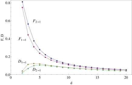
Figure 1: Optimal learning of a measurement device: we present the values of $D,F$ for different values of the dimension $d$. The squared dots represent the optimal learning from a single use ($1\to 1$ learning) while the round dots and triangles represent the optimal learning from two uses ($2\to 1$ learning).

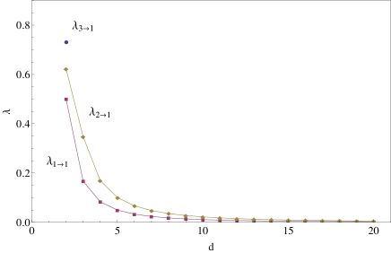
Figure 2: Optimal learning of a measurement device: we present the values of $\lambda$, the admixture of perfect replica to white noise in the produced measurement for different values of the dimension $d$. The squared dots represent the optimal learning from a single use ($1\to 1$ learning) while the diamonds represent the optimal learning from two uses ($2\to 1$ learning).

Due to Lemma 5 the replicated POVM has the following form:

$$G_{i}^{(U)} = \lambda E_{i}^{(U)}+(1-\lambda)\frac{1}{d}I$$

$$= \frac{dF-1}{d-1}U|i\rangle\langle i|U^{\dagger}+\frac{1-F}{d-1}I,$$

where the values of the coefficient $\lambda$ describing the random mixing of a perfect replica with a trivial measurement are depicted on Figure 2.

V.3 $3\to 1$ learning

In this section we consider a learning network, which exploits $3$ uses of the measurement device and produces a single replica:

$$\begin{aligned} \lx@xy@svg{\hbox{\raise 0.0pt\hbox{\kern 9.16656pt\hbox{\ignorespaces\ignorespaces\ignorespaces\hbox{\vtop{\kern 0.0pt\offinterlineskip\halign{\entry@#!@&&\entry@@#!@\cr&&&&&&&&&&&&\\&&&&&&&&&&&&\\&&&&&&&&&&&&\crcr}}}\ignorespaces{\hbox{\kern 0.0pt\raise 0.0pt\hbox{\hbox{\kern-3.0pt\raise 0.0pt\hbox{\hbox{\kern 3.0pt\raise 0.0pt\hbox{$\textstyle{}$}}}}}}}{\hbox{\kern 14.16656pt\raise 0.0pt\hbox{\hbox{\kern-3.0pt\raise 0.0pt\hbox{\hbox{\kern 3.0pt\raise 0.0pt\hbox{$\textstyle{}$}}}}}}}{\hbox{\kern 34.61299pt\raise 0.0pt\hbox{\hbox{\kern-3.0pt\raise 0.0pt\hbox{\hbox{\kern 3.0pt\raise 0.0pt\hbox{$\textstyle{}$}}}}}}}{\hbox{\kern 55.05942pt\raise 0.0pt\hbox{\hbox{\kern-3.0pt\raise 0.0pt\hbox{\hbox{\kern 3.0pt\raise 0.0pt\hbox{$\textstyle{}$}}}}}}}{\hbox{\kern 69.22598pt\raise 0.0pt\hbox{\hbox{\kern-3.0pt\raise 0.0pt\hbox{\hbox{\kern 3.0pt\raise 0.0pt\hbox{$\textstyle{}$}}}}}}}{\hbox{\kern 83.39255pt\raise 0.0pt\hbox{\hbox{\kern-3.0pt\raise 0.0pt\hbox{\hbox{\kern 3.0pt\raise 0.0pt\hbox{$\textstyle{}$}}}}}}}{\hbox{\kern 103.83897pt\raise 0.0pt\hbox{\hbox{\kern-3.0pt\raise 0.0pt\hbox{\hbox{\kern 3.0pt\raise 0.0pt\hbox{$\textstyle{}$}}}}}}}{\hbox{\kern 124.2854pt\raise 0.0pt\hbox{\hbox{\kern-3.0pt\raise 0.0pt\hbox{\hbox{\kern 3.0pt\raise 0.0pt\hbox{$\textstyle{}$}}}}}}}{\hbox{\kern 138.45197pt\raise 0.0pt\hbox{\hbox{\kern-3.0pt\raise 0.0pt\hbox{\hbox{\kern 3.0pt\raise 0.0pt\hbox{$\textstyle{}$}}}}}}}{\hbox{\kern 152.61853pt\raise 0.0pt\hbox{\hbox{\kern-3.0pt\raise 0.0pt\hbox{\hbox{\kern 3.0pt\raise 0.0pt\hbox{$\textstyle{}$}}}}}}}{\hbox{\kern 173.06496pt\raise 0.0pt\hbox{\hbox{\kern-3.0pt\raise 0.0pt\hbox{\hbox{\kern 3.0pt\raise 0.0pt\hbox{$\textstyle{}$}}}}}}}{\hbox{\kern 193.51138pt\raise 0.0pt\hbox{\hbox{\kern-2.5pt\raise 5.0pt\hbox{$\textstyle{6}$}}}}}{\hbox{\kern 198.51138pt\raise 0.0pt\hbox{\hbox{\kern 5.0pt\raise 0.0pt\hbox{$\textstyle{\hphantom{\;\;\;}}$}}}}}\ignorespaces\ignorespaces\ignorespaces\ignorespaces{}{\hbox{\lx@xy@droprule}}\ignorespaces{}{\hbox{\lx@xy@droprule}}{\hbox{\lx@xy@droprule}}{\hbox{\kern-9.16656pt\raise-29.26427pt\hbox{\hbox{\kern 5.0pt\raise 0.0pt\hbox{$\textstyle{\hphantom{\;\;\;}}$}}}}}\ignorespaces\ignorespaces\ignorespaces\ignorespaces{\hbox{\kern-4.16656pt\raise-43.8964pt\hbox{\hbox{\kern 0.0pt\raise 0.0pt\hbox{$\textstyle{\;\;\;}$}}}}}\ignorespaces\ignorespaces\ignorespaces\ignorespaces\ignorespaces\ignorespaces{\hbox{\lx@xy@droprule}}\ignorespaces\ignorespaces\ignorespaces\ignorespaces\ignorespaces{\hbox{\lx@xy@droprule}}\ignorespaces\ignorespaces\ignorespaces\ignorespaces\ignorespaces\ignorespaces{\hbox{\lx@xy@droprule}}\ignorespaces\ignorespaces\ignorespaces\ignorespaces\ignorespaces\ignorespaces\ignorespaces{\hbox{\lx@xy@droprule}}\ignorespaces{\hbox{\kern-9.16656pt\raise-24.7643pt\hbox{\hbox{\kern 0.0pt\raise-8.99994pt\hbox{$\textstyle{\hbox{\cirbuild@}}$}}}}}\ignorespaces{\hbox{\kern-9.16656pt\raise-63.0285pt\hbox{\hbox{\kern 0.0pt\raise 8.99994pt\hbox{$\textstyle{\hbox{\cirbuild@}}$}}}}}{\hbox{\kern 14.16656pt\raise-29.26427pt\hbox{\hbox{\kern-2.5pt\raise 5.0pt\hbox{$\textstyle{0}$}}}}}\ignorespaces\ignorespaces\ignorespaces\ignorespaces{}{\hbox{\lx@xy@droprule}}\ignorespaces{}{\hbox{\lx@xy@droprule}}{\hbox{\lx@xy@droprule}}{\hbox{\kern 19.16656pt\raise-29.26427pt\hbox{\hbox{\kern 0.0pt\raise 0.0pt\hbox{$\textstyle{\lx@xy@svgnested{\hbox{\raise 0.0pt\hbox{\kern 20.59523pt\hbox{{\hbox{\kern-10.2976pt\raise 0.0pt\hbox{\hbox{\kern 2.5pt\raise-4.46666pt\hbox{$\textstyle{\vphantom{\rule{0.0pt}{1.00006pt}\mathbf{E}^{(U)}}}$}}}}}{\hbox{\kern-10.29762pt\raise 0.0pt\hbox{\hbox{\kern 0.0pt\raise 0.0pt\hbox{\cirbuild@}}}}}\ignorespaces{\hbox{\kern-15.59523pt\raise 0.0pt\hbox{\hbox{\kern 0.0pt\raise-4.46666pt\hbox{$\textstyle{\mathbf{E}^{(U)}}$}}}}}\ignorespaces\ignorespaces\ignorespaces\ignorespaces\ignorespaces{\hbox{\kern-20.59523pt\raise 10.29762pt\hbox{\hbox{\kern 0.0pt\raise-4.46666pt\hbox{$\textstyle{\hphantom{\mathbf{E}^{(U)}}}$}}}}}\ignorespaces\ignorespaces\ignorespaces{\hbox{\lx@xy@droprule}}\ignorespaces\ignorespaces\ignorespaces\ignorespaces\ignorespaces{\hbox{\kern-20.59523pt\raise-10.29762pt\hbox{\hbox{\kern 0.0pt\raise-4.46666pt\hbox{$\textstyle{\hphantom{\mathbf{E}^{(U)}}}$}}}}}\ignorespaces\ignorespaces\ignorespaces{\hbox{\lx@xy@droprule}}\ignorespaces\ignorespaces\ignorespaces{\hbox{\kern-20.59523pt\raise 10.29762pt\hbox{\hbox{\kern 0.0pt\raise-4.46666pt\hbox{$\textstyle{\hphantom{\mathbf{E}^{(U)}}}$}}}}}\ignorespaces\ignorespaces\ignorespaces{\hbox{\kern-20.59523pt\raise-10.29762pt\hbox{\hbox{\kern 0.0pt\raise-4.46666pt\hbox{$\textstyle{\hphantom{\mathbf{E}^{(U)}}}$}}}}}\ignorespaces\ignorespaces\ignorespaces{\hbox{\lx@xy@droprule}}}}}}}$}}}}}\ignorespaces\ignorespaces\ignorespaces\ignorespaces{}{\hbox{\lx@xy@droprule}}\ignorespaces{}{\hbox{\lx@xy@droprule}}{\hbox{\lx@xy@droprule}}{\hbox{\kern 55.05942pt\raise-29.26427pt\hbox{\hbox{\kern-2.5pt\raise 5.0pt\hbox{$\textstyle{1}$}}}}}\ignorespaces\ignorespaces\ignorespaces\ignorespaces{}{\hbox{\hbox{\kern 0.0pt\raise-1.0pt\hbox{\lx@xy@droprule}}\hbox{\kern 0.0pt\raise 1.0pt\hbox{\lx@xy@droprule}}}}\ignorespaces{}{\hbox{\hbox{\kern 0.0pt\raise-1.0pt\hbox{\lx@xy@droprule}}\hbox{\kern 0.0pt\raise 1.0pt\hbox{\lx@xy@droprule}}}}{\hbox{\hbox{\kern 0.0pt\raise-1.0pt\hbox{\lx@xy@droprule}}\hbox{\kern 0.0pt\raise 1.0pt\hbox{\lx@xy@droprule}}}}{\hbox{\kern 60.05942pt\raise-29.26427pt\hbox{\hbox{\kern 5.0pt\raise 0.0pt\hbox{$\textstyle{\hphantom{\;\;\;}}$}}}}}\ignorespaces\ignorespaces\ignorespaces\ignorespaces{}{\hbox{\hbox{\kern 0.0pt\raise-1.0pt\hbox{\lx@xy@droprule}}\hbox{\kern 0.0pt\raise 1.0pt\hbox{\lx@xy@droprule}}}}\ignorespaces{}{\hbox{\hbox{\kern 0.0pt\raise-1.0pt\hbox{\lx@xy@droprule}}\hbox{\kern 0.0pt\raise 1.0pt\hbox{\lx@xy@droprule}}}}{\hbox{\hbox{\kern 0.0pt\raise-1.0pt\hbox{\lx@xy@droprule}}\hbox{\kern 0.0pt\raise 1.0pt\hbox{\lx@xy@droprule}}}}{\hbox{\kern 83.39255pt\raise-29.26427pt\hbox{\hbox{\kern-2.5pt\raise 5.0pt\hbox{$\textstyle{2}$}}}}}\ignorespaces\ignorespaces\ignorespaces\ignorespaces{}{\hbox{\lx@xy@droprule}}\ignorespaces{}{\hbox{\lx@xy@droprule}}{\hbox{\lx@xy@droprule}}{\hbox{\kern 88.39255pt\raise-29.26427pt\hbox{\hbox{\kern 0.0pt\raise 0.0pt\hbox{$\textstyle{\lx@xy@svgnested{\hbox{\raise 0.0pt\hbox{\kern 20.59523pt\hbox{{\hbox{\kern-10.2976pt\raise 0.0pt\hbox{\hbox{\kern 2.5pt\raise-4.46666pt\hbox{$\textstyle{\vphantom{\rule{0.0pt}{1.00006pt}\mathbf{E}^{(U)}}}$}}}}}{\hbox{\kern-10.29762pt\raise 0.0pt\hbox{\hbox{\kern 0.0pt\raise 0.0pt\hbox{\cirbuild@}}}}}\ignorespaces{\hbox{\kern-15.59523pt\raise 0.0pt\hbox{\hbox{\kern 0.0pt\raise-4.46666pt\hbox{$\textstyle{\mathbf{E}^{(U)}}$}}}}}\ignorespaces\ignorespaces\ignorespaces\ignorespaces\ignorespaces{\hbox{\kern-20.59523pt\raise 10.29762pt\hbox{\hbox{\kern 0.0pt\raise-4.46666pt\hbox{$\textstyle{\hphantom{\mathbf{E}^{(U)}}}$}}}}}\ignorespaces\ignorespaces\ignorespaces{\hbox{\lx@xy@droprule}}\ignorespaces\ignorespaces\ignorespaces\ignorespaces\ignorespaces{\hbox{\kern-20.59523pt\raise-10.29762pt\hbox{\hbox{\kern 0.0pt\raise-4.46666pt\hbox{$\textstyle{\hphantom{\mathbf{E}^{(U)}}}$}}}}}\ignorespaces\ignorespaces\ignorespaces{\hbox{\lx@xy@droprule}}\ignorespaces\ignorespaces\ignorespaces{\hbox{\kern-20.59523pt\raise 10.29762pt\hbox{\hbox{\kern 0.0pt\raise-4.46666pt\hbox{$\textstyle{\hphantom{\mathbf{E}^{(U)}}}$}}}}}\ignorespaces\ignorespaces\ignorespaces{\hbox{\kern-20.59523pt\raise-10.29762pt\hbox{\hbox{\kern 0.0pt\raise-4.46666pt\hbox{$\textstyle{\hphantom{\mathbf{E}^{(U)}}}$}}}}}\ignorespaces\ignorespaces\ignorespaces{\hbox{\lx@xy@droprule}}}}}}}$}}}}}\ignorespaces\ignorespaces\ignorespaces\ignorespaces{}{\hbox{\lx@xy@droprule}}\ignorespaces{}{\hbox{\lx@xy@droprule}}{\hbox{\lx@xy@droprule}}{\hbox{\kern 124.2854pt\raise-29.26427pt\hbox{\hbox{\kern-2.5pt\raise 5.0pt\hbox{$\textstyle{3}$}}}}}\ignorespaces\ignorespaces\ignorespaces\ignorespaces{}{\hbox{\hbox{\kern 0.0pt\raise-1.0pt\hbox{\lx@xy@droprule}}\hbox{\kern 0.0pt\raise 1.0pt\hbox{\lx@xy@droprule}}}}\ignorespaces{}{\hbox{\hbox{\kern 0.0pt\raise-1.0pt\hbox{\lx@xy@droprule}}\hbox{\kern 0.0pt\raise 1.0pt\hbox{\lx@xy@droprule}}}}{\hbox{\hbox{\kern 0.0pt\raise-1.0pt\hbox{\lx@xy@droprule}}\hbox{\kern 0.0pt\raise 1.0pt\hbox{\lx@xy@droprule}}}}{\hbox{\kern 129.2854pt\raise-29.26427pt\hbox{\hbox{\kern 5.0pt\raise 0.0pt\hbox{$\textstyle{\hphantom{\;\;\;}}$}}}}}\ignorespaces\ignorespaces\ignorespaces\ignorespaces{}{\hbox{\hbox{\kern 0.0pt\raise-1.0pt\hbox{\lx@xy@droprule}}\hbox{\kern 0.0pt\raise 1.0pt\hbox{\lx@xy@droprule}}}}\ignorespaces{}{\hbox{\hbox{\kern 0.0pt\raise-1.0pt\hbox{\lx@xy@droprule}}\hbox{\kern 0.0pt\raise 1.0pt\hbox{\lx@xy@droprule}}}}{\hbox{\hbox{\kern 0.0pt\raise-1.0pt\hbox{\lx@xy@droprule}}\hbox{\kern 0.0pt\raise 1.0pt\hbox{\lx@xy@droprule}}}}{\hbox{\kern 152.61853pt\raise-29.26427pt\hbox{\hbox{\kern-2.5pt\raise 5.0pt\hbox{$\textstyle{4}$}}}}}\ignorespaces\ignorespaces\ignorespaces\ignorespaces{}{\hbox{\lx@xy@droprule}}\ignorespaces{}{\hbox{\lx@xy@droprule}}{\hbox{\lx@xy@droprule}}{\hbox{\kern 157.61853pt\raise-29.26427pt\hbox{\hbox{\kern 0.0pt\raise 0.0pt\hbox{$\textstyle{\lx@xy@svgnested{\hbox{\raise 0.0pt\hbox{\kern 20.59523pt\hbox{{\hbox{\kern-10.2976pt\raise 0.0pt\hbox{\hbox{\kern 2.5pt\raise-4.46666pt\hbox{$\textstyle{\vphantom{\rule{0.0pt}{1.00006pt}\mathbf{E}^{(U)}}}$}}}}}{\hbox{\kern-10.29762pt\raise 0.0pt\hbox{\hbox{\kern 0.0pt\raise 0.0pt\hbox{\cirbuild@}}}}}\ignorespaces{\hbox{\kern-15.59523pt\raise 0.0pt\hbox{\hbox{\kern 0.0pt\raise-4.46666pt\hbox{$\textstyle{\mathbf{E}^{(U)}}$}}}}}\ignorespaces\ignorespaces\ignorespaces\ignorespaces\ignorespaces{\hbox{\kern-20.59523pt\raise 10.29762pt\hbox{\hbox{\kern 0.0pt\raise-4.46666pt\hbox{$\textstyle{\hphantom{\mathbf{E}^{(U)}}}$}}}}}\ignorespaces\ignorespaces\ignorespaces{\hbox{\lx@xy@droprule}}\ignorespaces\ignorespaces\ignorespaces\ignorespaces\ignorespaces{\hbox{\kern-20.59523pt\raise-10.29762pt\hbox{\hbox{\kern 0.0pt\raise-4.46666pt\hbox{$\textstyle{\hphantom{\mathbf{E}^{(U)}}}$}}}}}\ignorespaces\ignorespaces\ignorespaces{\hbox{\lx@xy@droprule}}\ignorespaces\ignorespaces\ignorespaces{\hbox{\kern-20.59523pt\raise 10.29762pt\hbox{\hbox{\kern 0.0pt\raise-4.46666pt\hbox{$\textstyle{\hphantom{\mathbf{E}^{(U)}}}$}}}}}\ignorespaces\ignorespaces\ignorespaces{\hbox{\kern-20.59523pt\raise-10.29762pt\hbox{\hbox{\kern 0.0pt\raise-4.46666pt\hbox{$\textstyle{\hphantom{\mathbf{E}^{(U)}}}$}}}}}\ignorespaces\ignorespaces\ignorespaces{\hbox{\lx@xy@droprule}}}}}}}$}}}}}\ignorespaces\ignorespaces\ignorespaces\ignorespaces{}{\hbox{\lx@xy@droprule}}\ignorespaces{}{\hbox{\lx@xy@droprule}}{\hbox{\lx@xy@droprule}}{\hbox{\kern 193.51138pt\raise-29.26427pt\hbox{\hbox{\kern-2.5pt\raise 5.0pt\hbox{$\textstyle{5}$}}}}}\ignorespaces\ignorespaces\ignorespaces\ignorespaces{}{\hbox{\hbox{\kern 0.0pt\raise-1.0pt\hbox{\lx@xy@droprule}}\hbox{\kern 0.0pt\raise 1.0pt\hbox{\lx@xy@droprule}}}}\ignorespaces{}{\hbox{\hbox{\kern 0.0pt\raise-1.0pt\hbox{\lx@xy@droprule}}\hbox{\kern 0.0pt\raise 1.0pt\hbox{\lx@xy@droprule}}}}{\hbox{\hbox{\kern 0.0pt\raise-1.0pt\hbox{\lx@xy@droprule}}\hbox{\kern 0.0pt\raise 1.0pt\hbox{\lx@xy@droprule}}}}{\hbox{\kern 198.51138pt\raise-29.26427pt\hbox{\hbox{\kern 5.0pt\raise 0.0pt\hbox{$\textstyle{\hphantom{\;\;\;}}$}}}}}\ignorespaces\ignorespaces\ignorespaces\ignorespaces{}{\hbox{\hbox{\kern 0.0pt\raise-1.0pt\hbox{\lx@xy@droprule}}\hbox{\kern 0.0pt\raise 1.0pt\hbox{\lx@xy@droprule}}}}\ignorespaces{}{\hbox{\hbox{\kern 0.0pt\raise-1.0pt\hbox{\lx@xy@droprule}}\hbox{\kern 0.0pt\raise 1.0pt\hbox{\lx@xy@droprule}}}}{\hbox{\hbox{\kern 0.0pt\raise-1.0pt\hbox{\lx@xy@droprule}}\hbox{\kern 0.0pt\raise 1.0pt\hbox{\lx@xy@droprule}}}}{\hbox{\kern-9.16656pt\raise-58.52853pt\hbox{\hbox{\kern 5.0pt\raise 0.0pt\hbox{$\textstyle{\hphantom{\;\;\;}}$}}}}}{\hbox{\kern 14.16656pt\raise-58.52853pt\hbox{\hbox{\kern-3.0pt\raise 0.0pt\hbox{\hbox{\kern 3.0pt\raise 0.0pt\hbox{$\textstyle{\ignorespaces\ignorespaces\ignorespaces\ignorespaces}$}}}}}}}\ignorespaces\ignorespaces\ignorespaces\ignorespaces{}{\hbox{\lx@xy@droprule}}\ignorespaces{}{\hbox{\lx@xy@droprule}}{\hbox{\lx@xy@droprule}}{\hbox{\kern 34.61299pt\raise-58.52853pt\hbox{\hbox{\kern-3.0pt\raise 0.0pt\hbox{\hbox{\kern 3.0pt\raise 0.0pt\hbox{$\textstyle{\ignorespaces\ignorespaces\ignorespaces\ignorespaces}$}}}}}}}\ignorespaces\ignorespaces\ignorespaces\ignorespaces{}{\hbox{\lx@xy@droprule}}\ignorespaces{}{\hbox{\lx@xy@droprule}}{\hbox{\lx@xy@droprule}}{\hbox{\kern 55.05942pt\raise-58.52853pt\hbox{\hbox{\kern-3.0pt\raise 0.0pt\hbox{\hbox{\kern 3.0pt\raise 0.0pt\hbox{$\textstyle{\ignorespaces\ignorespaces\ignorespaces\ignorespaces}$}}}}}}}\ignorespaces\ignorespaces\ignorespaces\ignorespaces{}{\hbox{\lx@xy@droprule}}\ignorespaces{}{\hbox{\lx@xy@droprule}}{\hbox{\lx@xy@droprule}}{\hbox{\kern 60.05942pt\raise-58.52853pt\hbox{\hbox{\kern 5.0pt\raise 0.0pt\hbox{$\textstyle{\hphantom{\;\;\;}}$}}}}}\ignorespaces\ignorespaces\ignorespaces\ignorespaces{}{\hbox{\lx@xy@droprule}}\ignorespaces{}{\hbox{\lx@xy@droprule}}{\hbox{\lx@xy@droprule}}\ignorespaces\ignorespaces{\hbox{\kern 65.05942pt\raise-43.89641pt\hbox{\hbox{\kern 0.0pt\raise 0.0pt\hbox{$\textstyle{\;\;\;}$}}}}}\ignorespaces\ignorespaces\ignorespaces\ignorespaces\ignorespaces{\hbox{\lx@xy@droprule}}\ignorespaces\ignorespaces\ignorespaces\ignorespaces\ignorespaces{\hbox{\lx@xy@droprule}}\ignorespaces\ignorespaces\ignorespaces\ignorespaces\ignorespaces{\hbox{\lx@xy@droprule}}\ignorespaces\ignorespaces\ignorespaces\ignorespaces\ignorespaces{\hbox{\lx@xy@droprule}}{\hbox{\kern 83.39255pt\raise-58.52853pt\hbox{\hbox{\kern-3.0pt\raise 0.0pt\hbox{\hbox{\kern 3.0pt\raise 0.0pt\hbox{$\textstyle{\ignorespaces\ignorespaces\ignorespaces\ignorespaces}$}}}}}}}\ignorespaces\ignorespaces\ignorespaces\ignorespaces{}{\hbox{\lx@xy@droprule}}\ignorespaces{}{\hbox{\lx@xy@droprule}}{\hbox{\lx@xy@droprule}}{\hbox{\kern 103.83897pt\raise-58.52853pt\hbox{\hbox{\kern-3.0pt\raise 0.0pt\hbox{\hbox{\kern 3.0pt\raise 0.0pt\hbox{$\textstyle{\ignorespaces\ignorespaces\ignorespaces\ignorespaces}$}}}}}}}\ignorespaces\ignorespaces\ignorespaces\ignorespaces{}{\hbox{\lx@xy@droprule}}\ignorespaces{}{\hbox{\lx@xy@droprule}}{\hbox{\lx@xy@droprule}}{\hbox{\kern 124.2854pt\raise-58.52853pt\hbox{\hbox{\kern-3.0pt\raise 0.0pt\hbox{\hbox{\kern 3.0pt\raise 0.0pt\hbox{$\textstyle{\ignorespaces\ignorespaces\ignorespaces\ignorespaces}$}}}}}}}\ignorespaces\ignorespaces\ignorespaces\ignorespaces{}{\hbox{\lx@xy@droprule}}\ignorespaces{}{\hbox{\lx@xy@droprule}}{\hbox{\lx@xy@droprule}}{\hbox{\kern 129.2854pt\raise-58.52853pt\hbox{\hbox{\kern 5.0pt\raise 0.0pt\hbox{$\textstyle{\hphantom{\;\;\;}}$}}}}}\ignorespaces\ignorespaces\ignorespaces\ignorespaces{}{\hbox{\lx@xy@droprule}}\ignorespaces{}{\hbox{\lx@xy@droprule}}{\hbox{\lx@xy@droprule}}\ignorespaces\ignorespaces{\hbox{\kern 134.2854pt\raise-43.89641pt\hbox{\hbox{\kern 0.0pt\raise 0.0pt\hbox{$\textstyle{\;\;\;}$}}}}}\ignorespaces\ignorespaces\ignorespaces\ignorespaces\ignorespaces{\hbox{\lx@xy@droprule}}\ignorespaces\ignorespaces\ignorespaces\ignorespaces\ignorespaces{\hbox{\lx@xy@droprule}}\ignorespaces\ignorespaces\ignorespaces\ignorespaces\ignorespaces{\hbox{\lx@xy@droprule}}\ignorespaces\ignorespaces\ignorespaces\ignorespaces\ignorespaces{\hbox{\lx@xy@droprule}}{\hbox{\kern 152.61853pt\raise-58.52853pt\hbox{\hbox{\kern-3.0pt\raise 0.0pt\hbox{\hbox{\kern 3.0pt\raise 0.0pt\hbox{$\textstyle{\ignorespaces\ignorespaces\ignorespaces\ignorespaces}$}}}}}}}\ignorespaces\ignorespaces\ignorespaces\ignorespaces{}{\hbox{\lx@xy@droprule}}\ignorespaces{}{\hbox{\lx@xy@droprule}}{\hbox{\lx@xy@droprule}}{\hbox{\kern 173.06496pt\raise-58.52853pt\hbox{\hbox{\kern-3.0pt\raise 0.0pt\hbox{\hbox{\kern 3.0pt\raise 0.0pt\hbox{$\textstyle{\ignorespaces\ignorespaces\ignorespaces\ignorespaces}$}}}}}}}\ignorespaces\ignorespaces\ignorespaces\ignorespaces{}{\hbox{\lx@xy@droprule}}\ignorespaces{}{\hbox{\lx@xy@droprule}}{\hbox{\lx@xy@droprule}}{\hbox{\kern 193.51138pt\raise-58.52853pt\hbox{\hbox{\kern-3.0pt\raise 0.0pt\hbox{\hbox{\kern 3.0pt\raise 0.0pt\hbox{$\textstyle{\ignorespaces\ignorespaces\ignorespaces\ignorespaces}$}}}}}}}\ignorespaces\ignorespaces\ignorespaces\ignorespaces{}{\hbox{\lx@xy@droprule}}\ignorespaces{}{\hbox{\lx@xy@droprule}}{\hbox{\lx@xy@droprule}}{\hbox{\kern 198.51138pt\raise-58.52853pt\hbox{\hbox{\kern 5.0pt\raise 0.0pt\hbox{$\textstyle{\hphantom{\;\;\;}}$}}}}}\ignorespaces\ignorespaces\ignorespaces\ignorespaces{}{\hbox{\lx@xy@droprule}}\ignorespaces{}{\hbox{\lx@xy@droprule}}{\hbox{\lx@xy@droprule}}\ignorespaces\ignorespaces{\hbox{\kern 203.51138pt\raise-29.26427pt\hbox{\hbox{\kern 0.0pt\raise 0.0pt\hbox{$\textstyle{\;\;\;}$}}}}}\ignorespaces\ignorespaces\ignorespaces\ignorespaces\ignorespaces{\hbox{\lx@xy@droprule}}\ignorespaces\ignorespaces\ignorespaces\ignorespaces\ignorespaces{\hbox{\lx@xy@droprule}}\ignorespaces\ignorespaces\ignorespaces\ignorespaces\ignorespaces{\hbox{\lx@xy@droprule}}\ignorespaces\ignorespaces\ignorespaces\ignorespaces\ignorespaces{\hbox{\lx@xy@droprule}}\ignorespaces}}}}\ignorespaces\end{aligned}\ . \textstyle{6} \textstyle{0} \textstyle{\mathbf{E}^{(U)}} \textstyle{1} \textstyle{2} \textstyle{\mathbf{E}^{(U)}} \textstyle{3} \textstyle{4} \textstyle{\mathbf{E}^{(U)}} \textstyle{5} \textstyle{6} \textstyle{0} \textstyle{\mathbf{E}^{(U)}} \textstyle{1} \textstyle{2} \textstyle{\mathbf{E}^{(U)}} \textstyle{3} \textstyle{4} \textstyle{\mathbf{E}^{(U)}} \textstyle{5}$$ (90)

In order to simplify the problem we restrict ourselves to the qubit case, that is we set $d=2$. The derivation of the optimal learning network turns out to be very involved although it follows the same lines as for the $2\to 1$ case. We made the calculations analytically with the help of a symbolic mathematical program.

The $3\to 1$ scenario deserves interest because the optimal solution does not allow a strategy having the $3$ uses of the measurement device in parallel. In other words the optimal strategy needs to be adaptive.

Let us consider the normalization condition for the generalized instrument $\{R_{i}\}$:

$$\sum_{ijkl}|jkl\rangle\langle jkl|_{531}\otimes R_{i,jkl}=I_{65}\otimes S_{43210}$$

$${\rm Tr}_{4}[S]=I_{3}\otimes T_{210}$$ (91)

This implies

$$\sum_{i}R_{i,jkl}=I_{6}\otimes\left\langle{kl}\right|S_{43210}\left|{kl}\right\rangle_{31}\quad\forall j,$$

$$\left\langle{kl}\right|{\rm Tr}_{4}[S]\left|{kl}\right\rangle=\left\langle{l}\right|T\left|{l}\right\rangle_{1}\quad\forall k.$$ (92)

From the relabeling symmetry $R_{i,jkl}=R_{\sigma(i),\sigma(j)\sigma(k)\sigma(l)}$ we have $\left\langle{kl}\right|S\left|{kl}\right\rangle=\left\langle{\sigma(k)\sigma(l)}\right|S\left|{\sigma(k)\sigma(l)}\right\rangle$, and consequently

$$\left\langle{kl}\right|{\rm Tr}_{4}[S]\left|{kl}\right\rangle_{31}=\frac{1}{d^{2}}{\rm Tr}_{431}[S]=:\widetilde{T}_{20},\quad\forall k,l.$$ (93)

This fact along with Eq. (91) allows us to conclude that

$${\rm Tr}_{4}[S]= {\rm Tr}_{4}\left[\sum_{kl}|kl\rangle\langle kl|_{31}\otimes\left\langle{kl}\right|S_{43210}\left|{kl}\right\rangle\right]=$$

$$\sum_{kl}|kl\rangle\langle kl|_{31}\otimes\widetilde{T}_{20}=I_{31}\otimes\widetilde{T}_{20}$$ (94)

which means that the first two uses can be in parallel. We notice that in general $\left\langle{kl}\right|S\left|{kl}\right\rangle=\left\langle{\sigma(k)\sigma(l)}\right|S\left|{\sigma(k)\sigma(l)}\right\rangle$ does not imply that $\left\langle{kl}\right|S\left|{kl}\right\rangle=\widetilde{S}$ is independent of $k,l$, but only that $\left\langle{kl}\right|S\left|{kl}\right\rangle=\widetilde{S}_{ab}$, where $a,b$ denotes the equivalence class of the couple $(k,l)$. Consequently, we cannot in general assume that all the examples can be used in parallel. In fact, the optimal learning network has the following causal structure

$$\begin{aligned} \lx@xy@svg{\hbox{\raise 0.0pt\hbox{\kern 9.16656pt\hbox{\ignorespaces\ignorespaces\ignorespaces\hbox{\vtop{\kern 0.0pt\offinterlineskip\halign{\entry@#!@&&\entry@@#!@\cr&&&&&&&&\\&&&&&&&&\\&&&&&&&&\crcr}}}\ignorespaces{\hbox{\kern-9.16656pt\raise 0.0pt\hbox{\hbox{\kern 5.0pt\raise 0.0pt\hbox{$\textstyle{\hphantom{\;\;\;}}$}}}}}\ignorespaces\ignorespaces\ignorespaces\ignorespaces{\hbox{\kern-4.16656pt\raise-34.39642pt\hbox{\hbox{\kern 0.0pt\raise 0.0pt\hbox{$\textstyle{\;\;\;}$}}}}}\ignorespaces\ignorespaces\ignorespaces\ignorespaces\ignorespaces\ignorespaces{\hbox{\lx@xy@droprule}}\ignorespaces\ignorespaces\ignorespaces\ignorespaces\ignorespaces{\hbox{\lx@xy@droprule}}\ignorespaces\ignorespaces\ignorespaces\ignorespaces\ignorespaces\ignorespaces{\hbox{\lx@xy@droprule}}\ignorespaces\ignorespaces\ignorespaces\ignorespaces\ignorespaces\ignorespaces\ignorespaces{\hbox{\lx@xy@droprule}}\ignorespaces{\hbox{\kern-9.16656pt\raise 4.49997pt\hbox{\hbox{\kern 0.0pt\raise-8.99994pt\hbox{$\textstyle{\hbox{\cirbuild@}}$}}}}}\ignorespaces{\hbox{\kern-9.16656pt\raise-73.29282pt\hbox{\hbox{\kern 0.0pt\raise 8.99994pt\hbox{$\textstyle{\hbox{\cirbuild@}}$}}}}}{\hbox{\kern 16.16653pt\raise 0.0pt\hbox{\hbox{\kern-2.5pt\raise 5.0pt\hbox{$\textstyle{0}$}}}}}\ignorespaces\ignorespaces\ignorespaces\ignorespaces{}{\hbox{\lx@xy@droprule}}\ignorespaces{}{\hbox{\lx@xy@droprule}}{\hbox{\lx@xy@droprule}}{\hbox{\kern 23.1665pt\raise 0.0pt\hbox{\hbox{\kern 0.0pt\raise 0.0pt\hbox{$\textstyle{\lx@xy@svgnested{\hbox{\raise 0.0pt\hbox{\kern 20.59523pt\hbox{{\hbox{\kern-10.2976pt\raise 0.0pt\hbox{\hbox{\kern 2.5pt\raise-4.46666pt\hbox{$\textstyle{\vphantom{\rule{0.0pt}{1.00006pt}\mathbf{E}^{(U)}}}$}}}}}{\hbox{\kern-10.29762pt\raise 0.0pt\hbox{\hbox{\kern 0.0pt\raise 0.0pt\hbox{\cirbuild@}}}}}\ignorespaces{\hbox{\kern-15.59523pt\raise 0.0pt\hbox{\hbox{\kern 0.0pt\raise-4.46666pt\hbox{$\textstyle{\mathbf{E}^{(U)}}$}}}}}\ignorespaces\ignorespaces\ignorespaces\ignorespaces\ignorespaces{\hbox{\kern-20.59523pt\raise 10.29762pt\hbox{\hbox{\kern 0.0pt\raise-4.46666pt\hbox{$\textstyle{\hphantom{\mathbf{E}^{(U)}}}$}}}}}\ignorespaces\ignorespaces\ignorespaces{\hbox{\lx@xy@droprule}}\ignorespaces\ignorespaces\ignorespaces\ignorespaces\ignorespaces{\hbox{\kern-20.59523pt\raise-10.29762pt\hbox{\hbox{\kern 0.0pt\raise-4.46666pt\hbox{$\textstyle{\hphantom{\mathbf{E}^{(U)}}}$}}}}}\ignorespaces\ignorespaces\ignorespaces{\hbox{\lx@xy@droprule}}\ignorespaces\ignorespaces\ignorespaces{\hbox{\kern-20.59523pt\raise 10.29762pt\hbox{\hbox{\kern 0.0pt\raise-4.46666pt\hbox{$\textstyle{\hphantom{\mathbf{E}^{(U)}}}$}}}}}\ignorespaces\ignorespaces\ignorespaces{\hbox{\kern-20.59523pt\raise-10.29762pt\hbox{\hbox{\kern 0.0pt\raise-4.46666pt\hbox{$\textstyle{\hphantom{\mathbf{E}^{(U)}}}$}}}}}\ignorespaces\ignorespaces\ignorespaces{\hbox{\lx@xy@droprule}}}}}}}$}}}}}\ignorespaces\ignorespaces\ignorespaces\ignorespaces{}{\hbox{\lx@xy@droprule}}\ignorespaces{}{\hbox{\lx@xy@droprule}}{\hbox{\lx@xy@droprule}}{\hbox{\kern 61.05933pt\raise 0.0pt\hbox{\hbox{\kern-2.5pt\raise 5.0pt\hbox{$\textstyle{1}$}}}}}\ignorespaces\ignorespaces\ignorespaces\ignorespaces{}{\hbox{\hbox{\kern 0.0pt\raise-1.0pt\hbox{\lx@xy@droprule}}\hbox{\kern 0.0pt\raise 1.0pt\hbox{\lx@xy@droprule}}}}\ignorespaces{}{\hbox{\hbox{\kern 0.0pt\raise-1.0pt\hbox{\lx@xy@droprule}}\hbox{\kern 0.0pt\raise 1.0pt\hbox{\lx@xy@droprule}}}}{\hbox{\hbox{\kern 0.0pt\raise-1.0pt\hbox{\lx@xy@droprule}}\hbox{\kern 0.0pt\raise 1.0pt\hbox{\lx@xy@droprule}}}}{\hbox{\kern 68.0593pt\raise 0.0pt\hbox{\hbox{\kern 5.0pt\raise 0.0pt\hbox{$\textstyle{\hphantom{\;\;\;}}$}}}}}\ignorespaces\ignorespaces\ignorespaces\ignorespaces{}{\hbox{\hbox{\kern 0.0pt\raise-1.0pt\hbox{\lx@xy@droprule}}\hbox{\kern 0.0pt\raise 1.0pt\hbox{\lx@xy@droprule}}}}\ignorespaces{}{\hbox{\hbox{\kern 0.0pt\raise-1.0pt\hbox{\lx@xy@droprule}}\hbox{\kern 0.0pt\raise 1.0pt\hbox{\lx@xy@droprule}}}}{\hbox{\hbox{\kern 0.0pt\raise-1.0pt\hbox{\lx@xy@droprule}}\hbox{\kern 0.0pt\raise 1.0pt\hbox{\lx@xy@droprule}}}}{\hbox{\kern 93.3924pt\raise 0.0pt\hbox{\hbox{\kern-3.0pt\raise 0.0pt\hbox{\hbox{\kern 3.0pt\raise 0.0pt\hbox{$\textstyle{}$}}}}}}}{\hbox{\kern 115.83879pt\raise 0.0pt\hbox{\hbox{\kern-3.0pt\raise 0.0pt\hbox{\hbox{\kern 3.0pt\raise 0.0pt\hbox{$\textstyle{}$}}}}}}}{\hbox{\kern 138.28519pt\raise 0.0pt\hbox{\hbox{\kern-2.5pt\raise 5.0pt\hbox{$\textstyle{6}$}}}}}{\hbox{\kern 145.28516pt\raise 0.0pt\hbox{\hbox{\kern 5.0pt\raise 0.0pt\hbox{$\textstyle{\hphantom{\;\;\;}}$}}}}}\ignorespaces\ignorespaces\ignorespaces\ignorespaces{}{\hbox{\lx@xy@droprule}}\ignorespaces{}{\hbox{\lx@xy@droprule}}{\hbox{\lx@xy@droprule}}{\hbox{\kern-9.16656pt\raise-39.52858pt\hbox{\hbox{\kern 5.0pt\raise 0.0pt\hbox{$\textstyle{\hphantom{\;\;\;}}$}}}}}{\hbox{\kern 16.16653pt\raise-39.52858pt\hbox{\hbox{\kern-2.5pt\raise 5.0pt\hbox{$\textstyle{2}$}}}}}\ignorespaces\ignorespaces\ignorespaces\ignorespaces{}{\hbox{\lx@xy@droprule}}\ignorespaces{}{\hbox{\lx@xy@droprule}}{\hbox{\lx@xy@droprule}}{\hbox{\kern 23.1665pt\raise-39.52858pt\hbox{\hbox{\kern 0.0pt\raise 0.0pt\hbox{$\textstyle{\lx@xy@svgnested{\hbox{\raise 0.0pt\hbox{\kern 20.59523pt\hbox{{\hbox{\kern-10.2976pt\raise 0.0pt\hbox{\hbox{\kern 2.5pt\raise-4.46666pt\hbox{$\textstyle{\vphantom{\rule{0.0pt}{1.00006pt}\mathbf{E}^{(U)}}}$}}}}}{\hbox{\kern-10.29762pt\raise 0.0pt\hbox{\hbox{\kern 0.0pt\raise 0.0pt\hbox{\cirbuild@}}}}}\ignorespaces{\hbox{\kern-15.59523pt\raise 0.0pt\hbox{\hbox{\kern 0.0pt\raise-4.46666pt\hbox{$\textstyle{\mathbf{E}^{(U)}}$}}}}}\ignorespaces\ignorespaces\ignorespaces\ignorespaces\ignorespaces{\hbox{\kern-20.59523pt\raise 10.29762pt\hbox{\hbox{\kern 0.0pt\raise-4.46666pt\hbox{$\textstyle{\hphantom{\mathbf{E}^{(U)}}}$}}}}}\ignorespaces\ignorespaces\ignorespaces{\hbox{\lx@xy@droprule}}\ignorespaces\ignorespaces\ignorespaces\ignorespaces\ignorespaces{\hbox{\kern-20.59523pt\raise-10.29762pt\hbox{\hbox{\kern 0.0pt\raise-4.46666pt\hbox{$\textstyle{\hphantom{\mathbf{E}^{(U)}}}$}}}}}\ignorespaces\ignorespaces\ignorespaces{\hbox{\lx@xy@droprule}}\ignorespaces\ignorespaces\ignorespaces{\hbox{\kern-20.59523pt\raise 10.29762pt\hbox{\hbox{\kern 0.0pt\raise-4.46666pt\hbox{$\textstyle{\hphantom{\mathbf{E}^{(U)}}}$}}}}}\ignorespaces\ignorespaces\ignorespaces{\hbox{\kern-20.59523pt\raise-10.29762pt\hbox{\hbox{\kern 0.0pt\raise-4.46666pt\hbox{$\textstyle{\hphantom{\mathbf{E}^{(U)}}}$}}}}}\ignorespaces\ignorespaces\ignorespaces{\hbox{\lx@xy@droprule}}}}}}}$}}}}}\ignorespaces\ignorespaces\ignorespaces\ignorespaces{}{\hbox{\lx@xy@droprule}}\ignorespaces{}{\hbox{\lx@xy@droprule}}{\hbox{\lx@xy@droprule}}{\hbox{\kern 61.05933pt\raise-39.52858pt\hbox{\hbox{\kern-2.5pt\raise 5.0pt\hbox{$\textstyle{3}$}}}}}\ignorespaces\ignorespaces\ignorespaces\ignorespaces{}{\hbox{\hbox{\kern 0.0pt\raise-1.0pt\hbox{\lx@xy@droprule}}\hbox{\kern 0.0pt\raise 1.0pt\hbox{\lx@xy@droprule}}}}\ignorespaces{}{\hbox{\hbox{\kern 0.0pt\raise-1.0pt\hbox{\lx@xy@droprule}}\hbox{\kern 0.0pt\raise 1.0pt\hbox{\lx@xy@droprule}}}}{\hbox{\hbox{\kern 0.0pt\raise-1.0pt\hbox{\lx@xy@droprule}}\hbox{\kern 0.0pt\raise 1.0pt\hbox{\lx@xy@droprule}}}}{\hbox{\kern 68.0593pt\raise-39.52858pt\hbox{\hbox{\kern 5.0pt\raise 0.0pt\hbox{$\textstyle{\hphantom{\;\;\;}}$}}}}}\ignorespaces\ignorespaces\ignorespaces\ignorespaces{}{\hbox{\hbox{\kern 0.0pt\raise-1.0pt\hbox{\lx@xy@droprule}}\hbox{\kern 0.0pt\raise 1.0pt\hbox{\lx@xy@droprule}}}}\ignorespaces{}{\hbox{\hbox{\kern 0.0pt\raise-1.0pt\hbox{\lx@xy@droprule}}\hbox{\kern 0.0pt\raise 1.0pt\hbox{\lx@xy@droprule}}}}{\hbox{\hbox{\kern 0.0pt\raise-1.0pt\hbox{\lx@xy@droprule}}\hbox{\kern 0.0pt\raise 1.0pt\hbox{\lx@xy@droprule}}}}{\hbox{\kern 93.3924pt\raise-39.52858pt\hbox{\hbox{\kern-2.5pt\raise 5.0pt\hbox{$\textstyle{4}$}}}}}\ignorespaces\ignorespaces\ignorespaces\ignorespaces{}{\hbox{\lx@xy@droprule}}\ignorespaces{}{\hbox{\lx@xy@droprule}}{\hbox{\lx@xy@droprule}}{\hbox{\kern 100.39236pt\raise-39.52858pt\hbox{\hbox{\kern 0.0pt\raise 0.0pt\hbox{$\textstyle{\lx@xy@svgnested{\hbox{\raise 0.0pt\hbox{\kern 20.59523pt\hbox{{\hbox{\kern-10.2976pt\raise 0.0pt\hbox{\hbox{\kern 2.5pt\raise-4.46666pt\hbox{$\textstyle{\vphantom{\rule{0.0pt}{1.00006pt}\mathbf{E}^{(U)}}}$}}}}}{\hbox{\kern-10.29762pt\raise 0.0pt\hbox{\hbox{\kern 0.0pt\raise 0.0pt\hbox{\cirbuild@}}}}}\ignorespaces{\hbox{\kern-15.59523pt\raise 0.0pt\hbox{\hbox{\kern 0.0pt\raise-4.46666pt\hbox{$\textstyle{\mathbf{E}^{(U)}}$}}}}}\ignorespaces\ignorespaces\ignorespaces\ignorespaces\ignorespaces{\hbox{\kern-20.59523pt\raise 10.29762pt\hbox{\hbox{\kern 0.0pt\raise-4.46666pt\hbox{$\textstyle{\hphantom{\mathbf{E}^{(U)}}}$}}}}}\ignorespaces\ignorespaces\ignorespaces{\hbox{\lx@xy@droprule}}\ignorespaces\ignorespaces\ignorespaces\ignorespaces\ignorespaces{\hbox{\kern-20.59523pt\raise-10.29762pt\hbox{\hbox{\kern 0.0pt\raise-4.46666pt\hbox{$\textstyle{\hphantom{\mathbf{E}^{(U)}}}$}}}}}\ignorespaces\ignorespaces\ignorespaces{\hbox{\lx@xy@droprule}}\ignorespaces\ignorespaces\ignorespaces{\hbox{\kern-20.59523pt\raise 10.29762pt\hbox{\hbox{\kern 0.0pt\raise-4.46666pt\hbox{$\textstyle{\hphantom{\mathbf{E}^{(U)}}}$}}}}}\ignorespaces\ignorespaces\ignorespaces{\hbox{\kern-20.59523pt\raise-10.29762pt\hbox{\hbox{\kern 0.0pt\raise-4.46666pt\hbox{$\textstyle{\hphantom{\mathbf{E}^{(U)}}}$}}}}}\ignorespaces\ignorespaces\ignorespaces{\hbox{\lx@xy@droprule}}}}}}}$}}}}}\ignorespaces\ignorespaces\ignorespaces\ignorespaces{}{\hbox{\lx@xy@droprule}}\ignorespaces{}{\hbox{\lx@xy@droprule}}{\hbox{\lx@xy@droprule}}{\hbox{\kern 138.28519pt\raise-39.52858pt\hbox{\hbox{\kern-2.5pt\raise 5.0pt\hbox{$\textstyle{5}$}}}}}\ignorespaces\ignorespaces\ignorespaces\ignorespaces{}{\hbox{\hbox{\kern 0.0pt\raise-1.0pt\hbox{\lx@xy@droprule}}\hbox{\kern 0.0pt\raise 1.0pt\hbox{\lx@xy@droprule}}}}\ignorespaces{}{\hbox{\hbox{\kern 0.0pt\raise-1.0pt\hbox{\lx@xy@droprule}}\hbox{\kern 0.0pt\raise 1.0pt\hbox{\lx@xy@droprule}}}}{\hbox{\hbox{\kern 0.0pt\raise-1.0pt\hbox{\lx@xy@droprule}}\hbox{\kern 0.0pt\raise 1.0pt\hbox{\lx@xy@droprule}}}}{\hbox{\kern 145.28516pt\raise-39.52858pt\hbox{\hbox{\kern 5.0pt\raise 0.0pt\hbox{$\textstyle{\hphantom{\;\;\;}}$}}}}}\ignorespaces\ignorespaces\ignorespaces\ignorespaces{}{\hbox{\hbox{\kern 0.0pt\raise-1.0pt\hbox{\lx@xy@droprule}}\hbox{\kern 0.0pt\raise 1.0pt\hbox{\lx@xy@droprule}}}}\ignorespaces{}{\hbox{\hbox{\kern 0.0pt\raise-1.0pt\hbox{\lx@xy@droprule}}\hbox{\kern 0.0pt\raise 1.0pt\hbox{\lx@xy@droprule}}}}{\hbox{\hbox{\kern 0.0pt\raise-1.0pt\hbox{\lx@xy@droprule}}\hbox{\kern 0.0pt\raise 1.0pt\hbox{\lx@xy@droprule}}}}{\hbox{\kern-9.16656pt\raise-68.79285pt\hbox{\hbox{\kern 5.0pt\raise 0.0pt\hbox{$\textstyle{\hphantom{\;\;\;}}$}}}}}{\hbox{\kern 16.16653pt\raise-68.79285pt\hbox{\hbox{\kern-3.0pt\raise 0.0pt\hbox{\hbox{\kern 3.0pt\raise 0.0pt\hbox{$\textstyle{\ignorespaces\ignorespaces\ignorespaces\ignorespaces}$}}}}}}}\ignorespaces\ignorespaces\ignorespaces\ignorespaces{}{\hbox{\lx@xy@droprule}}\ignorespaces{}{\hbox{\lx@xy@droprule}}{\hbox{\lx@xy@droprule}}{\hbox{\kern 38.61293pt\raise-68.79285pt\hbox{\hbox{\kern-3.0pt\raise 0.0pt\hbox{\hbox{\kern 3.0pt\raise 0.0pt\hbox{$\textstyle{\ignorespaces\ignorespaces\ignorespaces\ignorespaces}$}}}}}}}\ignorespaces\ignorespaces\ignorespaces\ignorespaces{}{\hbox{\lx@xy@droprule}}\ignorespaces{}{\hbox{\lx@xy@droprule}}{\hbox{\lx@xy@droprule}}{\hbox{\kern 61.05933pt\raise-68.79285pt\hbox{\hbox{\kern-3.0pt\raise 0.0pt\hbox{\hbox{\kern 3.0pt\raise 0.0pt\hbox{$\textstyle{\ignorespaces\ignorespaces\ignorespaces\ignorespaces}$}}}}}}}\ignorespaces\ignorespaces\ignorespaces\ignorespaces{}{\hbox{\lx@xy@droprule}}\ignorespaces{}{\hbox{\lx@xy@droprule}}{\hbox{\lx@xy@droprule}}{\hbox{\kern 68.0593pt\raise-68.79285pt\hbox{\hbox{\kern 5.0pt\raise 0.0pt\hbox{$\textstyle{\hphantom{\;\;\;}}$}}}}}\ignorespaces\ignorespaces\ignorespaces\ignorespaces{}{\hbox{\lx@xy@droprule}}\ignorespaces{}{\hbox{\lx@xy@droprule}}{\hbox{\lx@xy@droprule}}\ignorespaces\ignorespaces{\hbox{\kern 73.0593pt\raise-34.39642pt\hbox{\hbox{\kern 0.0pt\raise 0.0pt\hbox{$\textstyle{\;\;\;}$}}}}}\ignorespaces\ignorespaces\ignorespaces\ignorespaces\ignorespaces{\hbox{\lx@xy@droprule}}\ignorespaces\ignorespaces\ignorespaces\ignorespaces\ignorespaces{\hbox{\lx@xy@droprule}}\ignorespaces\ignorespaces\ignorespaces\ignorespaces\ignorespaces{\hbox{\lx@xy@droprule}}\ignorespaces\ignorespaces\ignorespaces\ignorespaces\ignorespaces{\hbox{\lx@xy@droprule}}{\hbox{\kern 93.3924pt\raise-68.79285pt\hbox{\hbox{\kern-3.0pt\raise 0.0pt\hbox{\hbox{\kern 3.0pt\raise 0.0pt\hbox{$\textstyle{\ignorespaces\ignorespaces\ignorespaces\ignorespaces}$}}}}}}}\ignorespaces\ignorespaces\ignorespaces\ignorespaces{}{\hbox{\lx@xy@droprule}}\ignorespaces{}{\hbox{\lx@xy@droprule}}{\hbox{\lx@xy@droprule}}{\hbox{\kern 115.83879pt\raise-68.79285pt\hbox{\hbox{\kern-3.0pt\raise 0.0pt\hbox{\hbox{\kern 3.0pt\raise 0.0pt\hbox{$\textstyle{\ignorespaces\ignorespaces\ignorespaces\ignorespaces}$}}}}}}}\ignorespaces\ignorespaces\ignorespaces\ignorespaces{}{\hbox{\lx@xy@droprule}}\ignorespaces{}{\hbox{\lx@xy@droprule}}{\hbox{\lx@xy@droprule}}{\hbox{\kern 138.28519pt\raise-68.79285pt\hbox{\hbox{\kern-3.0pt\raise 0.0pt\hbox{\hbox{\kern 3.0pt\raise 0.0pt\hbox{$\textstyle{\ignorespaces\ignorespaces\ignorespaces\ignorespaces}$}}}}}}}\ignorespaces\ignorespaces\ignorespaces\ignorespaces{}{\hbox{\lx@xy@droprule}}\ignorespaces{}{\hbox{\lx@xy@droprule}}{\hbox{\lx@xy@droprule}}{\hbox{\kern 145.28516pt\raise-68.79285pt\hbox{\hbox{\kern 5.0pt\raise 0.0pt\hbox{$\textstyle{\hphantom{\;\;\;}}$}}}}}\ignorespaces\ignorespaces\ignorespaces\ignorespaces{}{\hbox{\lx@xy@droprule}}\ignorespaces{}{\hbox{\lx@xy@droprule}}{\hbox{\lx@xy@droprule}}\ignorespaces\ignorespaces{\hbox{\kern 150.28516pt\raise-34.39642pt\hbox{\hbox{\kern 0.0pt\raise 0.0pt\hbox{$\textstyle{\;\;\;}$}}}}}\ignorespaces\ignorespaces\ignorespaces\ignorespaces\ignorespaces{\hbox{\lx@xy@droprule}}\ignorespaces\ignorespaces\ignorespaces\ignorespaces\ignorespaces{\hbox{\lx@xy@droprule}}\ignorespaces\ignorespaces\ignorespaces\ignorespaces\ignorespaces{\hbox{\lx@xy@droprule}}\ignorespaces\ignorespaces\ignorespaces\ignorespaces\ignorespaces{\hbox{\lx@xy@droprule}}\ignorespaces}}}}\ignorespaces\end{aligned}\ . \textstyle{0} \textstyle{\mathbf{E}^{(U)}} \textstyle{1} \textstyle{6} \textstyle{2} \textstyle{\mathbf{E}^{(U)}} \textstyle{3} \textstyle{4} \textstyle{\mathbf{E}^{(U)}} \textstyle{5} \textstyle{0} \textstyle{\mathbf{E}^{(U)}} \textstyle{1} \textstyle{6} \textstyle{2} \textstyle{\mathbf{E}^{(U)}} \textstyle{3} \textstyle{4} \textstyle{\mathbf{E}^{(U)}} \textstyle{5}$$ (95)

where the state of system $4$ depends on the classical outcome in system $3$ and $1$. The optimal value of $F[\boldsymbol{\mathcal{R}}]$ is approximately $0,87$ (we remind that for the $1\to 1$ learning we had $F=0,75$, while for the $2\to 1$ case we had $F=0,81$). The corresponding value of coefficient $\lambda$ (see Eqs.(49),(50)) are depicted on Fig. (2).

Remark 1

One can wonder whether without assuming any symmetry it is possible to find a non-symmetric parallel strategy $\{R_{i}\}$ that achieves the optimal value of $F[\boldsymbol{\mathcal{R}}]$. However we remind that for any strategy $\{R_{i}\}$ we can build a symmetric one with the same normalization, that is without spoiling the parallelism, and giving the same fidelity. Since the optimal symmetric network cannot be parallel, we have that any other optimal network has to be sequential as well.

VI Conclusions

We analyzed optimal learning of a measurement device. Our approach to the problem is based on the formalism of quantum combs and generalized quantum instruments, introduced in Refs. comblong ; memoryeff ; architecture . The original problem can be significantly simplified by utilizing the symmetries provided by the figure of merit. In particular, covariance and relabeling symmetry allow us to significantly decrease the number of parameters, without affecting the figure of merit. As a consequence of the symmetry of the learning network the replicated measurement can be seen as a random mixture of a perfect replica of the measurement device to be learnt with weight $\lambda$ and of a trivial measurement producing all possible outcomes with the same probability independently of the input state with weight $1-\lambda$. For $2\to 1$ and $3\to 1$ learning the first two uses of the unknown measurement device can be parallelized, and and this result can be generalized to $N\to 1$ learning. However, the optimal learning algorithm cannot be further parallelized, namely the examples exceeding the second one must be used sequentially. This feature is very unusual, and it occurs in few cases of quantum algorithms Watrousdiscrimini ; fiuramicu . For example, while the quantum part of Shor’s algorithm can be parallelized, Grover’s algorithm cannot, as was proved in Ref. zalka . Our results prove that quantum learning of a von Neumann measurement shares with Grover’s algorithm the impossibility of parallelizing without affecting optimality. The parallelization of the first two examples from this point of view is a curious exception.

An obvious extension of the work would be to study the scaling of the performance of the optimal learning strategy with respect to $N$. However, our results show that optimal learning networks with different $N$ do not share the same the initial steps. This means that the optimization of $N\rightarrow 1$ learning can not be done inductively building on the results from $N-1\rightarrow 1$ case. The complexity of the optimization in general case rises mainly due to the causal influence of steps of the learning strategy on the remaining part of the network, which is reflected in the recursive structure of the normalization constraints.

Appendix A Calculations for $2\to 1$ Learning

The explicit expression of $\Delta^{\nu}_{a,bc}$ in Eq. (88) is given by

$$\Delta_{x,xx}^{\alpha}=\begin{pmatrix}\frac{2}{d+1}&0\\ 0&0\end{pmatrix},\quad\Delta_{x,xy}^{\alpha}=\frac{1}{2}\begin{pmatrix}\frac{1}{d+1}&\frac{1}{\sqrt{d^{2}-1}}\\ \frac{1}{\sqrt{d^{2}-1}}&\frac{1}{d-1}\end{pmatrix},$$

$$\Delta_{x,yy}^{\alpha}=\Delta_{x,yz}^{\alpha}=0,\quad\Delta_{x,yx}^{\alpha}=\sigma_{z}\Delta_{x,xy}^{\alpha}\sigma_{z}$$

$$\Delta_{x,xx}^{\beta}=\frac{d-1}{d+1},\quad\Delta_{x,xy}^{\beta}=\Delta_{x,yx}^{\beta}=\frac{d}{2(d+1)},$$

$$\Delta_{x,yy}^{\beta}=1,\quad\Delta_{x,yz}^{\beta}=\frac{1}{2},$$

$$\Delta_{x,xx}^{\gamma}=\Delta_{x,yy}^{\gamma}=0,\quad\Delta_{x,xy}^{\gamma}=\Delta_{x,xy}^{\gamma}=\frac{d-2}{2(d-1)},$$

$$\Delta_{x,yz}^{\gamma}=\frac{1}{2}.$$ (96)

Introducing the notation

$$s_{x,xx}^{\nu}:=r_{x,xx}^{\nu} s_{x,xy}^{\nu}:=(d-1)r_{x,xy}^{\nu}$$

$$s_{x,yx}^{\nu}:=(d-1)r_{x,yx}^{\nu} s_{x,yy}^{\nu}:=(d-1)r_{x,yy}^{\nu}$$

$$s_{x,yz}^{\nu}:=(d-2)(d-1)r_{x,yz}^{\nu},$$ (97)

the figure of merit (V.2) becomes

$$F =F_{\alpha}+F_{\beta}+F_{\gamma}$$

$$F_{\nu}\equiv\sum_{(a,bc)\in\mathsf{L}}{\rm Tr}[\Delta_{a,bc}^{\nu}s_{a,bc}^{\nu}],\quad\nu\in\{\alpha,\beta\gamma\}$$ (98)

We express $R^{\prime}_{i,jk}$ through $R_{a,bc}$ $(a,bc)\in\mathsf{L}$ and Equation (39). Depending on $j=k$ or $j\neq k$ Eq. (83) is equivalent to the following relations

$$j=k\Rightarrow$$

$$s_{x,xx}^{\alpha}+s_{x,yy}^{\alpha}=\begin{pmatrix}t_{+}&0\\ 0&t_{-}\end{pmatrix}$$

$$s_{x,xx}^{\beta}+s_{x,yy}^{\beta}=t_{+}$$

$$s_{x,xx}^{\gamma}+s_{x,yy}^{\gamma}=t_{-}$$

$$j\neq k\Rightarrow$$

$$s_{x,xy}^{\alpha}+\sigma_{z}s_{x,xy}^{\alpha}\sigma_{z}+s_{x,yz}^{\alpha}=\begin{pmatrix}(d-1)t_{+}&0\\ 0&(d-1)t_{-}\end{pmatrix}$$

$$2s_{x,xy}^{\beta}+s_{x,yz}^{\beta}=(d-1)t_{+}$$ (99)

$$2s_{x,xy}^{\gamma}+s_{x,yz}^{\gamma}=(d-1)t_{-},$$ (100)

where we utilized Equation (86) implied by Lemma 6. We now derive the optimal learning network for a fixed value of $t_{+}$ (remember that $t_{-}=(1-d_{+}t_{+})/d_{-}$).

First we maximize $F_{\beta}$ and $F_{\gamma}$ for the case $d\geq 3$. Using the expressions for the $\Delta_{i,jk}^{\nu}$ from Eq. (A) we have:

$$F_{\beta}= \sum_{(a,bc)\in\mathsf{L}}{\rm Tr}[\Delta_{a,bc}^{\beta}s_{a,bc}^{\beta}]\leq\max(\Delta_{x,xx}^{\beta},\Delta_{x,yy}^{\beta})t_{+}+$$

$$+\max(\Delta_{x,xy}^{\beta},\Delta_{x,yz}^{\beta})(d-1)t_{+}=$$

$$=\Delta_{x,yy}^{\beta}t_{+}+\Delta_{x,yz}^{\beta}(d-1)t_{+}=$$

$$=t_{+}+\frac{(d-1)t_{+}}{2}=\frac{(d+1)t_{+}}{2}$$ (101)

and

$$F_{\gamma}= \sum_{(a,bc)\in\mathsf{L}}{\rm Tr}[\Delta_{a,bc}^{\gamma}s_{a,bc}^{\gamma}]\leq\max(\Delta_{x,xx}^{\gamma},\Delta_{x,yy}^{\gamma})t_{-}+$$

$$+\max(\Delta_{x,xy}^{\gamma},\Delta_{x,yz}^{\gamma})(d-1)t_{-}=$$

$$=\Delta_{x,yz}^{\gamma}(d-1)t_{-}=\frac{(d-1)t_{-}}{2}.$$ (102)

where we used the normalizations constraints (A). The upper bounds (A) and  (A) can be achieved by taking

$$s_{x,xx}^{\beta}=s_{x,xy}^{\beta}=s_{x,yx}^{\beta}=s_{x,xx}^{\gamma}=s_{x,xy}^{\gamma}=s_{x,yx}^{\gamma}=0,$$

$$s_{x,yy}^{\beta}=t_{+},\quad s_{x,yz}^{\beta}=(d-1)t_{+},$$

$$s_{x,yy}^{\gamma}=t_{-},\quad s_{x,yz}^{\gamma}=(d-1)t_{-}.$$

For $d=2$ the irreducible representation denoted by $\gamma$ and the $x,yz$ class do not exist and the optimization yields $s_{x,xy}^{\beta}=t_{+}(d-1)$.

Let us now consider $F_{\alpha}$ (in this case there is no difference between $d\geq 3$ and $d=2$). Based on the expression of $\Delta_{i,jk}^{\alpha}$ we have:

$$F_{\alpha}= \sum_{(a,bc)\in\mathsf{L}}{\rm Tr}[\Delta_{a,bc}^{\alpha}s_{a,bc}^{\alpha}]=$$

$${\rm Tr}[\Delta_{x,xx}^{\alpha}s_{x,xx}^{\alpha}]+{\rm Tr}[\Delta_{x,xy}^{\alpha}s_{x,xy}^{\alpha}]+{\rm Tr}[\Delta_{x,yx}^{\alpha}s_{x,yx}^{\alpha}]=$$

$${\rm Tr}\left[\begin{pmatrix}\frac{2}{d+1}&0\\ 0&0\end{pmatrix}s_{x,xx}^{\alpha}+\begin{pmatrix}\frac{1}{d+1}&\frac{1}{\sqrt{d^{2}-1}}\\ \frac{1}{\sqrt{d^{2}-1}}&\frac{1}{d-1}\end{pmatrix}s_{x,xy}^{\alpha}\right]\leq$$

$$\frac{2}{d+1}t_{+}+{\rm Tr}\left[\begin{pmatrix}\frac{1}{d+1}&\frac{1}{\sqrt{d^{2}-1}}\\ \frac{1}{\sqrt{d^{2}-1}}&\frac{1}{d-1}\end{pmatrix}s_{x,xy}^{\alpha}\right],$$ (103)

and the bound can be achieved by taking

$$s_{x,xx}^{\alpha}=\begin{pmatrix}t_{+}&0\\ 0&t_{-}\end{pmatrix}.$$ (104)

Let us now focus on the expression ${\rm Tr}[\Delta_{x,xy}^{\alpha}s_{x,xy}^{\alpha}]$. The normalization constraint (A) for the operator $s_{x,xy}^{\alpha}$ can be rewritten as:

$$s_{x,yz}^{\alpha,+,-}=s_{x,yz}^{\alpha,-,+}=0$$

$$s_{x,yz}^{\alpha,+,+}+2s_{x,xy}^{\alpha,+,+}=(d-1)t_{+}$$

$$s_{x,yz}^{\alpha,-,-}+2s_{x,xy}^{\alpha,-,-}=(d-1)t_{-},$$ (105)

where we denoted $s_{a,bc}^{\alpha,\pm,\pm}:=\left\langle{\pm}\right|s_{a,bc}^{\alpha}\left|{\pm}\right\rangle$. Then we have

$${\rm Tr}[\Delta_{x,xy}^{\alpha}s_{x,xy}^{\alpha}] =\frac{s_{x,xy}^{\alpha,+,+}}{d+1}+\frac{s_{x,xy}^{\alpha,+,-}}{\sqrt{d^{2}-1}}+$$

$$\frac{s_{x,xy}^{\alpha,-,+}}{\sqrt{d^{2}-1}}+\frac{s_{x,xy}^{\alpha,-,-}}{d-1}\leq$$

$$\frac{s_{x,xy}^{\alpha,+,+}}{d+1}+2\frac{\sqrt{s_{x,xy}^{\alpha,+,+}s_{x,xy}^{\alpha,-,-}}}{\sqrt{d^{2}-1}}+\frac{s_{x,xy}^{\alpha,-,-}}{d-1}\leq$$ (106)

$$\frac{(d-1)t_{+}}{2(d+1)}+\frac{\sqrt{(d-1)t_{+}t_{-}}}{\sqrt{d+1}}+\frac{t_{-}}{2}$$ (107)

where we used the positivity of the operator $s_{x,xy}^{\alpha}$ for the inequality (106) and the normalization (A) for the second inequality (107). The upper bound in Eq. (107) can be achieved by taking

$$s_{x,xy}^{\alpha}=\frac{(d-1)}{2}\begin{pmatrix}t_{+}&\sqrt{t_{+}t_{-}}\\ \sqrt{t_{+}t_{-}}&t_{-}\end{pmatrix}$$ (108)

Finally, combining the optimal values of $F_{\alpha}$, $F_{\beta}$, and $F_{\gamma}$ we have

$$F[\boldsymbol{\mathcal{R}}]=\frac{d^{2}+3d}{2(d+1)}t_{+}+\frac{\sqrt{(d-1)t_{+}t_{-}}}{\sqrt{d+1}}+\frac{d}{2}t_{-}$$ (109)

References

(1)
V. Vapnik, Statistical Learning Theory, Wiley-Interscience (1989), ISBN 0-471-03003-1.
(2)
M. Nielsen and I. Chuang,
Phys. Rev. Lett. 79, 321 324 (1997)
(3) M. Sasaki, A. Carlini, and R. Jozsa, Phys. Rev. A 64, 022317 (2001).
(4) M. Sasaki and A. Carlini, Phys. Rev. A 66,
22303 (2002).
(5) S Gammelmark and K Mølmer, New J. Phys. 11,
p. 3017 (2009).
(6)
L. K. Grover
Proceedings of the 28th Annual ACM Symposium on the Theory of Computing, (1996)
(7) A. Bisio, G. Chiribella, G. M. D’Ariano, S.
Facchini, and P. Perinotti, Phys. Rev. A 81, 32324 (2010).
(8)
G. Chiribella, G. M. D’Ariano, and P. Perinotti,
Phys. Rev. A 80, 022339 (2009)
(9)
G. Chiribella, G. M. D’Ariano, and P. Perinotti,
Phys. Rev. Lett. 101, 060401 (2008)
(10) G. Chiribella, G. M. D’Ariano, and P. Perinotti,
Phys. Rev. Lett. 101, 180501 (2008).
(11)
This is equivalent to a usage of a direct sum over the classical outcomes.
(12) For , this number is known as Bell number
.In the case the solution is provided by the sum for
of numbers of disjoint partitions of a set with
elements into subsets, which is the sum of Stirling numbers of the
second kind for .
(13)
A. W. Harrow, A. Hassidim, D. W. Leung, J. Watrous
Phys. Rev. A 81, 032339 (2010)
(14)
J. Fiurasek, M. Micuda
Phys. Rev. A 80 042312 (2009).