Spectral Action from Anomalies

Abstract:

Starting from a theory of fermions moving in a fixed gauge and gravitational background we implement the scale invariance of the theory. Upon quantization the theory is anomalous but the anomaly can be cancelled by the addition of another term to the action. This term comes out to be basically the Chamseddine Connes spectral action introduced in the context of noncommutative geometry. An alternative realization of the dilaton may involve a collective scalar mode of all fermions accumulated in a scale-noninvariant dilaton action. The entire spectral action describes gauge and Higgs fields coupled with gravity. Here this action is coupled with a dilaton and we discuss how it relates to the transition from the radiation to the electroweak broken phase via condensation of Higgs fields.

1 Introduction

The aim of this note is to show how, starting from a theory of fermions coupled to a gauge and gravitational background, it is possible to have the full bosonic action emerged. We do this using the spectral properties of the (generalized) Dirac operator, and in this respect this work can be seen in the framework of Connes and collaborators approach to the standard model [1, 2, 3, 4], as well as of Sakharov induced gravity [5] (for a modern review see [6]). Our starting point is a theory of fermions moving in a fixed background of gauge and scalar fields and a curved (Euclidean) spacetime. We focus on the scale invariance of the theory at the classical level. To quantize it we employ the spectral regularization, based on the cutoff of the eigenvalues of the Dirac operator. The regularization however is not preserved at the quantum level, and a scale anomaly is developed. There are two alternative ways to deal with quantum anomalies in local transformations [7]. On one hand the scale invariance can be restored by changing the measure in the path integral. This is tantamount to the addition to the fermionic action of another contribution, which renders the bosonic background interacting to the dilaton field. An alternative realization of the dilaton may involve a collective scalar mode of all fermions accumulated in a scale-noninvariant dilaton action. Accordingly the spectral action arises as a part of the fermion effective action divided into the scale non-invariant and scale invariant parts. It turns out that in both cases the resulting action is a modification of Chamseddine-Connes spectral action but with opposite signs. The latter is a purely spectral function of the gauged Dirac operator (and of a cutoff) which describes a gauge theory coupled with gravity, and in the presence of the Higgs mechanism.

The invariance by (local) scale transformation introduces in the theory another field whereas the collective dilaton mode of fermions appears after their partial bosonization as a consequence of scale non-invariance. The dilaton effective potential has been calculated by us and in the last section we discuss how it relates to the transition from the radiation phase with zero v.e.v. of Higgs fields and massless particles to the electroweak broken phase via condensation of Higgs fields. It is proven that only the second way to interpret the spectral action with collective field of dilaton can provide the above mentioned phase transition with EW symmetry breaking during Universe evolution.

The first six Sections of these proceedings will mostly follow reference [8], although with a somewhat different point of view. The material in Sec.7 has not been previously published.

2 Fermions in a Fixed Background

Our starting point is a theory in which we have some matter fields, represented by fermions transforming under some (reducible) representation a gauge group, such as the standard model group $SU(3)\times SU(2)\times U(1)$. We need not specify the group for the moment. The fermions will be spinors belonging to some Hilbert space $\cal H$ which we assume to be “chiral”, i.e. split into a left and a right:

$${\cal H}={\cal H}_{L}\oplus{\cal H}_{R}$$ (1)

A generic matter field will therefore be a spinor

$$\Psi=\begin{pmatrix}\Psi_{L}\\ \Psi_{R}\end{pmatrix}$$ (2)

and in this representation the chirality operator, which we call $\gamma$ is a two by two diagonal matrix with plus and minus one eigenvalues. The two components are spinors themselves and we are not indicating the gauge indices, nor the flavor indices. We will assume that the fermions come in a number of identical (apart from the mass) generations.

The fermions are given a dynamics coupling them to a background field. This coupling is performed by a classical action which we schematically write as

$$S_{F}=\left\langle\Psi\right|D\left|\Psi\right\rangle$$ (3)

where

$$D=D_{0}+A$$ (4)

is an operator on $\cal H$ which will call always the Dirac operator, although the formalism we are building is more general and there may be “Dirac operators” which do not resemble at all the one introduced for the Dirac equation.

The Dirac operator, acting of spinors is again a matrix and we have split into a “free and gravitational” part and a “gauge coupling” part. We will see in a moment the reason for this (rather inaccurate) terminology.

We start from

$$D_{0}=\begin{pmatrix}\gamma^{\mu}\partial_{\mu}&M\\ M^{\dagger}&\gamma^{\mu}\partial_{\mu}\end{pmatrix}$$ (5)

Where $M$ contains all masses (and mixings) of the fermions and the $\gamma$ are those relative to a possibly curved spacetime. In this case the fermions are coupled to the gravitational fixed background given by the metric

$$g^{\mu\nu}=\frac{1}{2}\{\gamma^{\mu},\gamma^{\nu}\}$$ (6)

The matrix $A$ represents instead a fixed gauge background, and the interaction of the spinors with it. We emphasize that at this stage we are just describing the classical dynamics of fermions in a fixed background. We are deliberately vague as to the detail of the model at this stage, not discussing important elements of the theory, like chirality or charge conjugation. The scheme presented here is largely independent on the details of the model. In particular it applies to the standard model, especially in the approach based on noncommutative geometry introduced by Connes and briefly discussed below.

3 Fields, Hilbert Spaces, Dirac Operators and the (Non)commutative Geometry of Spacetime

We have introduced a (Euclidean) spacetime. And therefore implicitly the algebra $\cal A$ of complex valued continuous functions of this space time. There is in fact a one-to one correspondence between (topological Hausdorff) spaces and commutative $C^{*}$-algebras, i.e. associative normed algebras with an involution and a norm satisfying certain properties. This is the content of the Gelfand-Naimark theorem [9, 10], which describes the topology of space in terms of the algebras. In physicists terms we may say the properties of a space are encoded in the continuous fields defined on them. This concept, and its generalization to noncommutative algebras is one of the starting points of Connes noncommutative geometry programme [1]. The programme aims at the transcription of the usual concepts of differential geometry in algebraic terms and a key role of this programme is played by a spectral triple, which is composed by an algebra acting as operators on a Hilbert space and a (generalized) Dirac operator. In our case we have these ingredients, but we have to consider instead of the algebra of continuous complex valued function, matrix valued functions. The underlying space in this case is still the ordinary spacetime, technically the algebra is “Morita equivalent” to the commutative algebra, but the formalism is built in a general way so to be easily generalizable to the truly noncommutative case, when the underlying space may not be an ordinary geometry.

The spectral triple contains the information on the geometry of spacetime. The algebra as we said is dual to the topology, and the Dirac operator enables the translation of the metric and differential structure of spaces in an algebraic form. There is no room in these proceedings to describe this programme, and we refer to the literature for details [1, 11, 10, 12].

Within this general programme a key role is played by Connes’ approach to the standard model. This is the attempt to understand which kind of (noncommutative) geometry gives rise to the standard model of elementary particles coupled with gravity. The roots of this approach is to have the Higgs appear naturally as the “vector” boson of the internal noncommutative degrees of freedom [13, 14, 2]. The most complete formulation of this approach is given by the spectral action, which in its most recent form is presented in [4].

The fermionic part of this action is (3), while the bosonic part is basically the regularized sum of the eigenvalues of the Dirac operator. We will see how this action can fe inferred (with some little modifications) from the fermionic action $S_{F}$ and the need to preserve scale invariance.

4 Scale invariance of the Fermionic Action

So far we are in the presence of a classical theory of matter fields moving in a fixed background. The objects involved in the writing of the action have physical dimensions. Introduce a scale necessary for measurements, for example an unit of length $\ell$, then it is possible to measure volumes as $\ell^{-4}$, masses and the Dirac operator in general as $\ell^{-1}$ and so on.

The classical action is invariant under a change of this scale, after all is amounts to just a change of units of measurement. Recall that we have not yet introduced $\hbar$. In principle this change of scale could also be local, and this would be H. Weyl original “gauge” theory. We therefore have a scale transformation symmetry:

$$x^{\mu} \to {\rm e}^{\phi}x^{\mu}$$

$$\psi \to {\rm e}^{-\frac{3}{2}\phi}\psi$$

$$D \to {\rm e}^{-\frac{1}{2}\phi}D{\rm e}^{-\frac{1}{2}\phi}$$ (7)

where $\phi$ is a real parameter which for the moment we take to be constant. Note that since the rescaling involves also the matrix part of $D$, we must also rescale the masses of the fermions. In the absence of a dimensional scale, is an exact symmetry of the classical theory.

We now proceed to quantize the theory. It can be proven [15] that if the classical theory is invariant, the measure in the quantum path integral is not. We have an anomaly: a classical theory is invariant against a symmetry transformation, but the quantum theory, due to unavoidable regularization, does not possess this symmetry anymore. If also the quantum theory is required to be symmetric then the symmetry can be restored by the addition of extra terms in the action. A textbook introduction to anomalies can be found in [15]. The notion of scale anomaly is attached to the dilatation of both coordinates, fields and mass-like parameters according to their dimensionalities, Eq. (7). Evidently, in the absence of UV divergences, there is no scale anomaly which therefore can be correlated to rescaling of a cutoff in the theory. In the case when the dilatation is not constant, $\phi$ becomes a quantum field called the dilaton. The dilaton of this kind has been investigated in the context of the spectral action in [16].

We remark that there is also an alternative realization of the dilaton as a collective scalar mode of all fermions accumulated in a scale-noninvariant dilaton action. The corresponding spectral action has an opposite sign and will be discussed later on.

In both approaches we start from the partition function

$$Z(D)=\int[{\rm d}\psi][{\rm d}\bar{\psi}]e^{-S_{\psi}}=\det\left(\frac{D}{\mu}\right)$$ (8)

where a normalization scale $\mu$ is introduced and the last equality is formal because the expression is divergent and needs regularizing. The writing of the fermionic action in this form (as a Pfaffian) is instrumental in the solution of the fermion doubling problem in Connes approach to the standard model [17, 18, 4]. In fact we need in principle two regulators:

• $\mu$ which may be treated as an infrared cutoff when having a discrete spectrum;

• an ultraviolet cutoff $\Lambda$ in order to tame the short distance infinities.

We will regularize the theory in the ultraviolet using a procedure introduced by one of us, Bonora and Gamboa-Saravi in [19, 20, 21] but leaving a room for a normalization scale $\mu$. The energy cutoff is enforced by considering only the first $N$ eigenvalues of $D$. Consider the projector

$$P_{N}=\sum_{n=1}^{N}\left|\lambda_{n}\right\rangle\left\langle\lambda_{n}\right|;\quad N=\max n\ \mbox{such that}\ \lambda_{n}\leq\Lambda$$ (9)

where $\lambda_{n}$ are the eigenvalues of $D$ in increasing order (repeated according to possible multiplicities), $\left|\lambda_{n}\right\rangle$ a corresponding orthonormal basis, and the integer $N$ is a function of the cutoff. This means that we are effectively using the $N^{\mathrm{th}}$ eigenvalue as cutoff. Therefore this number and the corresponding spectral density depends on coefficient functions of the Dirac operator, $N=N(D)$.

In the framework of noncommutative geometry this is the most natural cutoff procedure, although it was introduced before the introduction of the standard model in noncommutative geometry. It makes no reference in principle to the underlying structure of spacetime, and it is based purely on spectral data, thus is perfectly adequate to Connes’ programme. This form of regularization could be also used for field theory which cannot be described on an ordinary spacetime, as long as there is a Dirac operator, or generically a wave operator, with a discrete spectrum.

We define the regularized partition function

$$Z_{\mu}(D) = \prod_{n=1}^{N}\frac{\lambda_{n}}{\mu}=\det\left(\mbox{1 \kern-5.89996pt{\rm l}}-P_{N}+P_{N}\frac{D}{\mu}P_{N}\right)$$ (10)

$$= \det\left(\mbox{1 \kern-5.89996pt{\rm l}}-P_{N}+P_{N}\frac{D}{\Lambda}P_{N}\right)\det\left(\mbox{1 \kern-5.89996pt{\rm l}}-P_{N}+\frac{\Lambda}{\mu}P_{N}\right)=Z_{\Lambda}(D)\det\left(\mbox{1 \kern-5.89996pt{\rm l}}-P_{N}+\frac{\Lambda}{\mu}P_{N}\right).$$

In this way we can define the fermionic action in an intrinsic way.

The regularized partition function $Z_{\Lambda}$ has a well defined meaning. Expressing $\psi$ and $\bar{\psi}$ as

$$\psi=\sum_{n=1}^{\infty}a_{n}\left|\lambda_{n}\right\rangle;\qquad\bar{\psi}=\sum_{n=1}^{\infty}b_{n}\left|\lambda_{n}\right\rangle$$ (11)

with $a_{n}$ and $b_{n}$ anticommuting (Grassman) quantities. Then $Z_{\Lambda}$ becomes (performing the integration over Grassman variables for the last step)

$$Z_{\Lambda}(D)=\int\prod_{n=1}^{N}\dfrac{{\rm d}a_{n}{\rm d}b_{n}}{\Lambda}{\rm e}^{-\sum_{n=1}^{N}b_{n}\lambda_{n}a_{n}}=\det\left(D_{N}\right)$$ (12)

where we defined

$$D_{N}=1-P_{N}+P_{N}\frac{D}{\Lambda}P_{N}.$$ (13)

In the basis in which $D/\Lambda$ is diagonal it corresponds to set to $\Lambda$ all eigenvalues larger than $\Lambda$. Note that $D_{N}$ is dimensionless and depends on $\Lambda$ both explicitly and intrinsically via the dependence of $N$ and $P_{N}$.

It is possible to give an explicit functional expression to the projector in terms of the cutoff:

$$P_{N}=\Theta\left(1-\frac{D^{2}}{\Lambda^{2}}\right)=\int\limits_{-\infty}^{\infty}{\rm d}\alpha\,\frac{1}{2\pi{\rm i}(\alpha-{\rm i}\epsilon)}{\rm e}^{{\rm i}\alpha\big{(}1-\frac{D^{2}}{\Lambda^{2}}\big{)}}$$ (14)

where $\Theta$ is the Heaviside step function. This integral is well defined for a compactified space volume and therefore in the presence of the infrared cutoff which can be identified with $\mu$. Actually $N$ depends also on the infrared cutoff, and the number of dimensions. It goes as $\sim\left(\frac{\Lambda}{\mu}\right)^{d}$.

5 Cancellation of the Anomaly and the Bosonic Action

Let’s perform the first scenario and restore scale invariance. The action $S_{F}$ is invariant under (7) but the partition function is not, the reason for this is the fact that the regularization procedure is not scale invariant. The cancellation of the anomaly then proceeds via a change of measure, which is equivalent to the addition of another term to the action. This term compensates the change in the measure due to the regularization, but being in an exponential form, can also be seen as another addition to the action, so that the final partition function is invariant. This calculation has been performed in [22] in the QCD context, and applied to gravity in [23].

Let us see in a very heuristic way, with $\phi$ constant, why the effective action $S_{\mathrm{eff}}$ is nothing but the spectral action with the function $\chi$ being a sharp cutoff. In this case $N$ is just a number of eigenvalues smaller that $\Lambda$, and thereby

$$\>{\rm Tr}\,\chi\left(\frac{D^{2}}{\Lambda^{2}}\right)=\>{\rm Tr}\,\Theta\left(1-\frac{D^{2}}{\Lambda^{2}}\right)=\>{\rm Tr}\,P_{N}=N(\Lambda,\ D).$$ (15)

It can be written in the latter form provided that we take into account the functional dependence $N=N(\Lambda,\ D)$. It is worth recalling again that the integer $N$ depends on the cutoff $\Lambda$, on the Dirac operator $D$ and also on the function $\chi$ which we have chosen to be a sharp cutoff.

Then the compensating term – the effective action, will be defined by

$${Z_{\mathrm{inv}}}_{\mu}(D)=Z_{\mu}(D)\int{\rm d}\phi\,{\rm e}^{-S_{\mathrm{anom}}}$$ (16)

where the effective action will be depending on $N$, and hence the cutoff $\Lambda$, and on $\phi$. Define

$$Z_{\mathrm{inv}\mu}(D)=\int{\rm d}\phi Z_{\mu}({\rm e}^{-\frac{1}{2}\phi}D{\rm e}^{-\frac{1}{2}\phi})=\int{\rm d}\phi Z_{\mu}(D_{\phi});\qquad D_{\phi}\equiv{\rm e}^{-\frac{1}{2}\phi}D{\rm e}^{-\frac{1}{2}\phi},$$ (17)

then

$$S_{\mathrm{anom}}=\log Z_{\mu}(D)Z_{\mu}^{-1}(D_{\phi})$$ (18)

Let us assign

$$Z_{t}=Z_{\mu}(D_{t\phi})$$ (19)

therefore $Z_{0}=Z_{\mu}(D)$ and

$${Z_{\mathrm{inv}}}_{\mu}(D)Z^{-1}_{\mu}(D)=\int{\rm d}\phi\frac{Z_{1}}{Z_{0}}$$ (20)

and hence

$$S_{\mathrm{anom}}=-\int_{0}^{1}{\rm d}t\partial_{t}\log Z_{t}=-\int_{0}^{1}{\rm d}t\frac{\partial_{t}Z_{t}}{Z_{t}}$$ (21)

We have the following relation that can easily proven

$$\partial_{t}Z_{t}=\partial_{t}\det\left(\frac{D_{t\phi}}{\mu}\right)_{N} = \phi Z_{t}\left(-1+\Lambda^{2}\log\frac{\Lambda^{2}}{\mu^{2}}\partial_{\Lambda^{2}}\right)\>{\rm tr}\,P_{N},$$ (22)

and therefore

$$S_{\mathrm{anom}} = \int_{0}^{1}{\rm d}t\,\phi\left(1-\Lambda^{2}\log\frac{\Lambda^{2}}{\mu^{2}}\partial_{\Lambda^{2}}\right)\>{\rm Tr}\,\Theta\left(1-\frac{D_{t\phi}^{2}}{\Lambda^{2}}\right)$$ (23)

$$= \int_{0}^{1}{\rm d}t\,\phi\left(1-\Lambda^{2}\log\frac{\Lambda^{2}}{\mu^{2}}\partial_{\Lambda^{2}}\right)N(\Lambda,\ D_{t\phi}).\$$

6 The Spectral Action

For $\phi=0$ this is basically the Chamseddine-Connes Spectral Action introduced in [3] together with the fermionic action (3). More precisely the bosonic part of the spectral action is

$$\>{\rm Tr}\,\chi\left(\frac{D^{2}}{\Lambda^{2}}\right)$$ (24)

where $\chi$ is a generic cutoff function, which in our case is a sharp cutoff at energy $\Lambda$,

$$\chi(x)=\left\{\begin{array}[]{cc}0{}&x<0\\ 1{}&x\in[0,1]\\ 0{}&x>1\end{array}\right.$$ (25)

consequence of the sharp cutoff on the eigenvalues used in (9). The bosonic spectral action so introduced is always finite by its nature, it is purely spectral and it depends on the cutoff $\Lambda$. In the original work of Chamseddine and Connes the bosonic and fermion parts of the action were treated differently. The fermionic action on the contrary is divergent, and will require renormalization. It is formulated as an usual integral. In the philosophy of noncommutative geometry usual integrals can be interpreted as a regularized trace, the Dixmier trace:

$$\int{\rm d}xf=\>{\rm Tr}\,_{\omega}|D|^{-4}f$$ (26)

where the Dixmier trace of an operator $O$ with eigenvalues $o_{n}$ (ordered in decreasing order, repeated in case of degeneracy) is:

$$\>{\rm Tr}\,_{\omega}O=\lim_{N\to\infty}\frac{1}{\log N}\sum_{n=0}^{N}o_{n}$$ (27)

The integral/Dixmier trace has however to be regularized. We have seen as the cancellation of the anomaly brings the two actions on the same footing, albeit with a modification of the bosonic part. It must be mentioned that already in [24] the two actions are “unified” in the bosonic action with the addition of the projection on the fermionic field to the covariant Dirac operator. This reproduces the full spectral action with some additional non linear terms for the fermions, which could have to do with fermionic masses.

To obtain the standard model take as algebra the product of the algebra of functions on spacetime times a finite dimensional matrix algebra

$$\mathcal{A}=C({\mathbb{R}}^{4})\otimes{\mathcal{A}}_{F}$$ (28)

Likewise the Hilbert space is the product of fermions times a finite dimensional space which contains all matter degrees of freedom, and also the Dirac operator contains a continuous part and a discrete one

$$\mathcal{H}={\mathrm{Sp}({\mathbb{R}}^{4})\otimes{\mathcal{H}}_{F}}$$ (29)

and the Dirac operator

$$D_{0}=\gamma^{\mu}\partial_{\mu}\otimes\mathbb{I}+\gamma\otimes D_{F}$$ (30)

In its most recent form due to Chamseddine, Connes and Marcolli [4] a crucial role is played by the mathematical requirements that the noncommutative algebra satisfies the requirements to be a manifold. Then the internal algebra, is almost uniquely derived to be

$${\mathcal{A}}_{F}={\mathbb{C}}\oplus{\mathbb{H}}\oplus M_{3}({\mathbb{C}})$$ (31)

Then the bosonic spectral action can be evaluated at one loop using standard heath kernel techniques [25] and the final result gives the full action of the standard model coupled with gravity. We restrain from writing it since it takes more than one page in the original paper [4]. In the process however one does not need to input the mass of the Higgs, which comes out as a prediction. Its value comes out to be $\sim 170\mathrm{GeV}$. A small value experimentally disfavoured. It must be said however that the present form of the model needs unification of the three coupling constant at a single energy point (given by $\Lambda$). The model also contains nonstandard gravitational terms (quadratic in the curvature), which are currently being investigated for their cosmological consequences [26, 27].

Technically the canonical bosonic spectral action is a sum of residues, and can be expanded in a power series in terms of $\Lambda^{-1}$ as

$$S_{B}=\sum_{n}f_{n}\,a_{n}(D^{2}/\Lambda^{2})$$

where the $f_{n}$ are the momenta of $\chi$

$$f_{0} = \int_{0}^{\infty}{\rm d}x\,x\chi(x)$$

$$f_{2} = \int_{0}^{\infty}{\rm d}x\,\chi(x)$$

$$f_{2n+4} = (-1)^{n}\partial^{n}_{x}\chi(x)\bigg{|}_{x=0}\ \ n\geq 0$$

the $a_{n}$ are the Seeley-de Witt coefficients which vanish for $n$ odd. For $D^{2}$ of the form

$$D^{2}=g^{\mu\nu}\partial_{\mu}\partial_{\nu}\mbox{1 \kern-5.89996pt{\rm l}}+\alpha^{\mu}\partial_{\mu}+\beta$$

defining

$$\omega_{\mu} = \frac{1}{2}g_{\mu\nu}\left(\alpha^{\nu}+g^{\sigma\rho}\Gamma^{\nu}_{\sigma\rho}\mbox{1 \kern-5.89996pt{\rm l}}\right)$$

$$\Omega_{\mu\nu} = \partial_{\mu}\omega_{\nu}-\partial_{\nu}\omega_{\mu}+[\omega_{\mu},\omega_{\nu}]$$

$$E = \beta-g^{\mu\nu}\left(\partial_{\mu}\omega_{\nu}+\omega_{\mu}\omega_{\nu}-\Gamma^{\rho}_{\mu\nu}\omega_{\rho}\right)$$

then

$$a_{0} = \frac{\Lambda^{4}}{16\pi^{2}}\int{\rm d}x^{4}\sqrt{g}\>{\rm tr}\,\mbox{1 \kern-5.89996pt{\rm l}}_{F}$$

$$a_{2} = \frac{\Lambda^{2}}{16\pi^{2}}\int{\rm d}x^{4}\sqrt{g}\>{\rm tr}\,\left(-\frac{R}{6}+E\right)$$

$$a_{4} = \frac{1}{16\pi^{2}}\frac{1}{360}\int{\rm d}x^{4}\sqrt{g}\>{\rm tr}\,(-12\nabla^{\mu}\nabla_{\mu}R+5R^{2}-2R_{\mu\nu}R^{\mu\nu}$$

$$+2R_{\mu\nu\sigma\rho}R^{\mu\nu\sigma\rho}-60RE+180E^{2}+60\nabla^{\mu}\nabla_{\mu}E+30\Omega_{\mu\nu}\Omega^{\mu\nu})$$

$\>{\rm tr}\,$ is the trace over the inner indices of the finite algebra $\mathcal{A}_{F}$ and in $\Omega$ and $E$ are contained the gauge degrees of freedom including the gauge stress energy tensors and the Higgs, which is given by the inner fluctuations of $D$.

In our case for $\phi$ constant, after performing the integration we find

$$S_{\mathrm{anom}} = \int_{0}^{\phi}{\rm d}t^{\prime}\sum_{n}{\rm e}^{(4-n)t^{\prime}}\left(1-\Lambda^{2}\log\frac{\Lambda^{2}}{\mu^{2}}\partial_{\Lambda^{2}}\right)a_{n}f_{n}$$ (32)

$$= \frac{1}{8}(e^{4\phi}-1)a_{0}\left(1-2\Lambda^{2}\log\frac{\Lambda^{2}}{\mu^{2}}\right)+\frac{1}{2}(e^{2\phi}-1)a_{2}\left(1-\Lambda^{2}\log\frac{\Lambda^{2}}{\mu^{2}}\right)+\phi a_{4}.$$

There are just some numerical corrections to the first two Seeley-de Witt coefficients due to the integration in $t\phi$ and a choice of normalization scale $\mu$.

We notice that the alternative way of treatment of the scale degree of freedom as a collective field leads to precisely the opposite sign of the dilaton action $S_{anom}\to S_{coll}=-S_{anom}$. Indeed the bosonization in scale variable can be represented as,

$$Z_{\mu}(D)=Z_{\mathrm{inv},\mu}(D)\int{\rm d}\phi\,{\rm e}^{-S_{\mathrm{coll}}};\quad Z_{\mathrm{inv}\mu}(D)=\int{\rm d}\phi Z^{-1}_{\mu}(D_{\phi})$$ (33)

then

$$S_{\mathrm{coll}}=\log Z^{-1}_{\mu}(D)Z_{\mu}(D_{\phi})=-S_{anom},$$ (34)

(cf. to (18)) .

7 The Dilaton and the effective potential

The full analysis of the model coupled with a dynamical dilaton is under way and will be published elsewhere. Nevertheless it is already possible to say something on the interplay between the dilaton and the Higgs, and in particular the effective potential. This can be used to characterize cosmic evolution right after inflation starts. In particular, it may open the ways to describe the transition from the radiation phase with massless particles to the EW symmetry breaking phase with spontaneous mass generation due to condensation of Higgs fields.

7.1 Mass generation from Higgs-dilaton potential during cosmic evolution

We will consider in the following only the potential terms relative to the complex Higgs doublet $H$ and the dilaton $\phi$. The quadratic term of the Higgs potential comes from the $a_{2}$ term of (32), while the quartic one comes from the $a_{4}$ one. In this way we can derive the form effective Higgs-dilaton potential. To focus on this goal we reduce the joint effective Higgs-dilaton (HD) potential including only the real scalar component $H$ of the Higgs doublet $(H_{1},H_{2})\to(0,H)$ subject to condensation. After performing renormalization the general form of the HD potential is expected to be,

$$V=V_{0}+Ae^{4\phi}+BH^{2}e^{2\phi}-CH^{4}(\phi+\phi_{0})+EH^{2},$$ (35)

where depending on the normalization scale $\mu$ of fermion effective action compared with the cutoff $\Lambda$ one can get any sign of the coefficients $A(\Lambda,\mu),B(\Lambda,\mu)\gtrless 0$. Evidently the constant $\phi_{0}$ can be eliminated by shifting the field $\phi\to\phi-\phi_{0}$ and rescaling the constants $A,B$. Thus in general both signs and modules of these constants $A,B$ don’t have any a priori values. As to the constant $C$, if the dilaton serves for restoration of conformal symmetry as an independent field then the conformal anomaly coefficient $C<0$ (see [8]). On the other hand, a composite dilaton made of fermions [22] has an anomalous part of the potential of the opposite sign with $C>0$. Therefore the sign of $C$ characterizes the nature of the dilaton field: elementary or composite one. In this Section we are interested in evolution of fields $\phi,H$ and correspondingly neglect the additional cosmological constant $V_{0}$. Thus for our purpose the potential has four arbitrary parameters $A,B,C,E$ and $\phi_{0}=0$.

We would like to apply the HD potential for description of cosmic evolution and select out of the acceptable signs and modules of the coefficients which can provide the evolution from a symmetric phase to the EW symmetry breaking phase with spontaneous mass generation due to condensation of Higgs fields. Thus one has to inquire about whether the HD potential has local minimums and what are the restrictions on the arbitrary coefficients which provide the existence of such minimums.

Accordingly we are going to investigate all possible critical points of this potential depending on the values of its coefficients. Without loss of generality one can impose $C>0$. For the opposite sign of $C$ the set of critical points can be found by reflection $V\to-V$. One can see, that $V$ has no any critical points at $H=0$. Let us perform the coordinate transformation to the variable $\eta$,

$$H^{2} = \eta e^{2\phi}$$ (36)

Such a transformation is non-degenerate at $H\neq 0$ and preserves all the information about extremal properties of our potential.

In the new variables the potential takes the form,

$$V=e^{4\phi}\left(A+B\eta-C\phi\eta^{2}\right)+Ee^{2\phi}\eta.$$ (37)

Critical point coordinates obey the following equations,

$$2A+B\eta-\frac{C}{2}\eta^{2} = 0$$ (38)

$$\left(\frac{2C\eta}{E}\right)\phi-\frac{B}{E} = e^{-2\phi}$$ (39)

with the additional requirement $\eta>0$ .

From the equation (38) we immediately find,

$$\eta_{1,2}={\frac{4A}{-B\pm\sqrt{{B}^{2}+4\,AC}}}.$$ (40)

It is known (for a quick introduction see e.g. [28]), that the equation of a type $ax+b=p^{cx+d}~{}~{}a,c\neq 0$, can be exactly solved in terms of the Lambert $W(z)$ function [29]. By definition, it is a solution of the equation,

$$z=W(z)e^{W(z)}$$ (41)

The function $We^{W}$ is not injective and $W$ is multivalued (except for 0). If we look for real-valued $W$ then the relation (41) is defined only for $x\geq 1/e$, and is double-valued on $(-1/e,0)$.

Let us introduce the notation $W_{0}(x)$ for the upper branch. It is defined at $-1/e\leq x<\infty$ and it is monotonously increasing from -1 to $+\infty$. The lower branch is usually denoted $W_{-1}(x)$. It is defined only on $-1/e\leq x<0$ and it is monotonously decreasing from -1 to $-\infty$.

In these terms the general solution of (39) is given by,

$$\phi=\frac{1}{2}W\left(\frac{Ee^{-\frac{B}{\eta C}}}{\eta C}\right)+{\frac{B}{2\eta\,C}}$$ (42)

Since we have two values of $\eta$ and the real $W$ is double-valued, then the maximal number of critical points is four. However $\eta$ must be positive and real, and $\phi$ must be real. From these requirements one obtains the restrictions on the coefficients, which provide an existence of each critical point.

We shall denote our critical points as $(m,n)$. Here the first index $m$ marks the sign $\pm$ and corresponds to the type of a chosen $\eta$ from (40). Index $n$ ranges over $-1,0$ and corresponds to the chosen branch of $W$ function. We specify a type of each critical point with the help of the Hessian matrix eigenvalues and find the following results for the acceptable composition of coefficient signs.

We seek for combinations of signs of the coefficients $A,B,C,E$ which provide a minimum triggering the spontaneous EW symmetry breaking at a final stage of cosmic evolution. There are 11 combinations of signs which are forbidden as they don’t provide the existence of a local minimum.

sign (A)	sign(B)	sign(C)	sign(E)
$\pm$	$\pm$	+	+
-	-	+	-
-	$\pm$	-	$\pm$
+	+	-	$\pm$

Only five combinations of signs can support the required minimum.

sign (A)	sign(B)	sign(C)	sign(E)
+	$+$	+	-
+	-	+	-
-	$+$	+	-
+	-	-	$+$
+	-	-	$-$

7.2 Transition from symmetric phase to Electroweak symmetry breaking phase and choice of signs

Now let’s examine the possibility of scenario when at the first stage of the Universe evolution one deals with a massless world with the vanishing v.e.v. of the Higgs field $\langle H_{in}\rangle=0$ (symmetric phase). Thus we adopt that every initial point $(\phi_{in},H_{in}=0)$ for starting evolution is acceptable if the function $V|_{\phi=\phi_{in}}(H)$ has a local minimum at $H=0$ and if we can roll down from the initial point to the final one which is a local minimum corresponding to the Higgs phase. We have listed five combinations of signs of the parameters $A$, $B$, $C$, $E$ which provide the existence of the local minimum . Nevertheless not all of these combinations support the above transition scenario. Indeed one can prove that this scenario can be realized only for positive $A,B,C$ and negative $E$. For this case the solution for minimum belongs to the class $(+,-1)$ and the minimum (final-stage) coordinates are given by,

$$\eta_{fin} = {\frac{4A}{-B+\sqrt{{B}^{2}+4\,AC}}}>0,$$ (43)

$$\phi_{fin} = \frac{1}{2}W_{-1}\left(\frac{Ee^{-\frac{B}{\eta_{fin}C}}}{\eta_{fin}C}\right)+{\frac{B}{2\eta_{fin}\,C}}.$$ (44)

The requirement for $\phi$ to be real leads to,

$${E_{min}<E<0,~{}~{}~{}~{}~{}E_{min}\equiv-C\eta_{fin}\exp\left\{-1+\frac{B}{\eta_{fin}C}\right\}}$$ (45)

The additional bounds exist on the coefficients,

$$Be^{2\phi_{in}}+E>0,$$ (46)

to guarantee that the initial point is in the symmetric phase. Evidently the phase transition point during evolution appears for $\phi_{crit}=(1/2)\ln(-E/B)<\phi_{in}$. It can be shown that $\phi_{fin}<\phi_{crit}<0$ and therefore $B+E>0$. We remark that the latter inequality entails $|E_{min}|>|E|$ . We summarize our finding in Fig. 1.

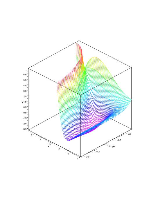
Figure 1: View of the effective Higgs-dilaton potential in the vicinity of its two symmetric local minima: $H=H_{m}=2.29$ and $\phi=\phi_{m}=-0.72$. Colored lines represent the sections of the plot of the potential by the surfaces of constant $\phi$ and constant $H$. Parameters are taken as follows: $A=1$, $B=2.1$, $C=0.2$, $E=-2$.

8 Conclusions

The main conclusions of this paper are:

• The bosonic spectral action can be provided by restoration of scale invariance in the fermion world or

• the bosonic spectral action can emerge from scale non-invariance of fermion world in terms of composite dilation; the two effective potentials differ in sign;

• the requirement to trigger EW breaking phase transition during evolution to the Higgs potential minimum gives a favor to the composite nature of dilaton.

- [1] A. Connes, Noncommutative Geometry, Academic Press, 1984.
- [2] A. Connes and J. Lott, “Particle Models and Noncommutative Geometry (Expanded Version),” Nucl. Phys. Proc. Suppl. 18B (1991) 29.
- [3] A. H. Chamseddine and A. Connes, “The spectral action principle,” Commun. Math. Phys. 186, 731 (1997) [arXiv:hep-th/9606001].
- [4] A. H. Chamseddine, A. Connes and M. Marcolli, “Gravity and the standard model with neutrino mixing,” Adv. Theor. Math. Phys. 11 (2007) 991 [arXiv:hep-th/0610241].
- [5] A. D. Sakharov, “Vacuum quantum fluctuations in curved space and the theory of gravitation,” Sov. Phys. Dokl. 12 (1968) 1040 [Dokl. Akad. Nauk Ser. Fiz. 177 (1967 SOPUA,34,394.1991 GRGVA,32,365-367.2000) 70].
- [6] M. Visser, “Sakharov’s induced gravity: A modern perspective,” Mod. Phys. Lett. A 17 (2002) 977 [arXiv:gr-qc/0204062].
- [7] A. A. Andrianov and Yu. V. Novozhilov, “Gauge Fields and Correspondence Principle,” Theor. Math. Phys. 67, 448 (1986) [Teor. Mat. Fiz. 67, 198 (1986)].
- [8] A. A. Andrianov and F. Lizzi, “Bosonic Spectral Action Induced from Anomaly Cancelation,” JHEP 1005 (2010) 057 [arXiv:1001.2036 [hep-th]].
- [9] J. M. G. Fell and R. S. Doran, Representations of ∗-Algebras, Locally Compact Groups and Banach ∗-Algebraic Bundles, Academic Press, (1988).
- [10] J.M. Gracia-Bondia, J.C. Varilly, H. Figueroa, Elements of Noncommutative Geometry, Birkhauser, 2000.
- [11] G. Landi, An Introduction to Noncommutative Spaces and their Geometries, Springer Lecture Notes in Physics 51, Springer Verlag (Berlin Heidelberg) 1997. arXiv:hep-th/9701078.
- [12] J. Madore, “An Introduction To Noncommutative Differential Geometry and its Physical Applications,” Lond. Math. Soc. Lect. Note Ser. 257 (2000) 1.
- [13] J. Madore, “Kaluza-Klein Aspects Of Noncommutative Geometry,” In *Chester 1988, Proceedings, Differential geometric methods in theoretical physics* 243-252.
- [14] M. Dubois-Violette, R. Kerner and J. Madore, “Noncommutative Differential Geometry Of Matrix Algebras,” J. Math. Phys. 31 (1990) 316.
- [15] K. Fujikawa, H. Suzuki, Path Integrals And Quantum Anomalies, Oxford university Press, 2004.
- [16] A. H. Chamseddine and A. Connes, “Scale invariance in the spectral action,” J. Math. Phys. 47 (2006) 063504 [arXiv:hep-th/0512169].
- [17] F. Lizzi, G. Mangano, G. Miele and G. Sparano, “Fermion Hilbert space and fermion doubling in the noncommutative geometry approach to gauge theories,” Phys. Rev. D 55, 6357 (1997) [arXiv:hep-th/9610035].
- [18] J. M. Gracia-Bondia, B. Iochum and T. Schucker, “The standard model in noncommutative geometry and fermion doubling,” Phys. Lett. B 416, 123 (1998) [arXiv:hep-th/9709145].
- [19] A. A. Andrianov, L. Bonora and R. Gamboa-Saravi, “Regularized Functional Integral For Fermions And Anomalies,” Phys. Rev. D 26, 2821 (1982).
- [20] A. A. Andrianov and L. Bonora, “Finite - Mode Regularization Of The Fermion Functional Integral,” Nucl. Phys. B 233, 232 (1984).
- [21] A. A. Andrianov and L. Bonora, “Finite Mode Regularization Of The Fermion Functional Integral. 2,” Nucl. Phys. B 233, 247 (1984).
- [22] A. A. Andrianov, V. A. Andrianov, V. Y. Novozhilov and Yu. V. Novozhilov, “Joint Chiral and Conformal Bosonization in QCD and the Linear Sigma Model,” Phys. Lett. B 186 (1987) 401.
- [23] Y. V. Novozhilov and D. V. Vassilevich, “Induced Quantum Conformal Gravity,” Phys. Lett. B 220 (1989) 36.
- [24] A. Sitarz, “Spectral action and neutrino mass,” Europhys. Lett. 86 (2009) 10007 [arXiv:0808.4127 [math-ph]].
- [25] D. V. Vassilevich, “Heat kernel expansion: User’s manual,” Phys. Rept. 388, 279 (2003) [arXiv:hep-th/0306138].
- [26] W. Nelson and M. Sakellariadou, “Cosmology and the Noncommutative approach to the Standard Model,” arXiv:0812.1657 [hep-th].
- [27] M. Marcolli and E. Pierpaoli, “Early Universe models from Noncommutative Geometry,” arXiv:0908.3683 [hep-th].
- [28] http://en.wikipedia.org/wiki/Lambertfunction .
- [29] Lambert, J. H. ”Observations variae in Mathesin Puram.” Acta Helvitica, physico-mathematico-anatomico-botanico-medica 3, 128-168, 1758. Euler, L. ”De serie Lambertina Plurimisque eius insignibus proprietatibus.” Acta Acad. Scient. Petropol. 2, 29-51, 1783.
- [30] F. Bezrukov, A. Magnin, M. Shaposhnikov and S. Sibiryakov, “Higgs inflation: consistency and generalisations,” JHEP 1101, 016 (2011) [arXiv:1008.5157 [hep-ph]].