Probing the entanglement and locating knots in ring polymers: a comparative study of different arc closure schemes

Abstract

The interplay between the topological and geometrical properties of a polymer ring can be clarified by establishing the entanglement trapped in any portion (arc) of the ring. The task requires to close the open arcs into a ring, and the resulting topological state may depend on the specific closure scheme that is followed. To understand the impact of this ambiguity in contexts of practical interest, such as knot localization in a ring with non trivial topology, we apply various closure schemes to model ring polymers. The rings have the same length and topological state (a trefoil knot) but have different degree of compactness. The comparison suggests that a novel method, termed the minimally-interfering closure, can be profitably used to characterize the arc entanglement in a robust and computationally-efficient way. This closure method is finally applied to the knot localization problem which is tackled using two different localization schemes based on top-down or bottom-up searches.

I Introduction

It is known that the global topological state of a ring polymer affects its salient physical properties such as its size  desCloizeux:1981:J-Phys-Lett ; Moore:2004:PNAS sedimentation velocity, gel-electrophoretic mobility Stasiak:1996:Nature:8906784 ; Weber_et_al_2006_Biophys_J ; Orlandini_et_al_2010_PRE , resistance to mechanical stretching Saitta_et_al:1999:Nature or the behaviour under spatial confinement  Marenduzzo:2009:Proc-Natl-Acad-Sci-U-S-A:20018693 .

While a comprehensive understanding of this phenomenon is still lacking, it is often explicitly or implicitly acknowledged that topology-dependent physical properties arise because of a sophisticated interplay of polymer geometry and topology. In other words, the global topological state affects the average geometrical properties of the polymer, which in turn directly impact various physical properties such as those mentioned above.

A vivid illustration of this relationship is offered by the mechanical resistance of a knotted polymer that is pulled at both ends. The breaking force depends on the topological state of the polymer. Indeed, the rupture point is invariably in correspondence of the knot Saitta_et_al:1999:Nature which is progressively tightened by the pulling action (as all fishermen know for the case of a knotted fishing line).

The above example highlights a very important player in the relationship between the topological, geometrical and physical properties of a ring polymer (or a polymer with constrained ends), namely the degree of localization of the topologically-entangled region Orlandini_et_al_2009:Phys-Bio . For example, recent simulations have shown that the delocalization of “knots” in a linear DNA filament is very important to allow its tranlocation through a pore (as in viral DNA ejected from the viral capsid) avoiding plug-like obstructions Marenduzzo:2009:Proc-Natl-Acad-Sci-U-S-A:20018693 .

Locating the knotted portion of the polymer is straightforward when the knot is tight, but is otherwise highly challenging. Generally speaking, to accomplish this task one needs to establish the degree/type of entanglement “trapped” in any portion, or arc, of the ring polymer and then select the shortest arc(s) whose trapped entanglement matches the global topology of the ring. The entanglement trapped in a given arc is identified by establishing the topology state of an auxiliary ring obtained by suitably joining the two arc ends.

The difficulty of this scheme lies in the fact that several viable arc closure (end-joining) schemes can be used and they can result in different knots being measured on the same arc. This is especially the case for rings under geometrical confinement Millett_2005_Macromol ; Orlandini&Whittington:2007:Rev-Mod_Phys ; Marcone:2007:PRE .

While the above-mentioned ambiguity is ultimately unavoidable, it is important to ascertain how severe it is in contexts of practical interest. This question, motivates the present study where we use and compare several closure schemes to characterize the entanglement trapped in portions of three model ring polymers with the same length and knotted state (trefoil knot) but with different degree of compactness and hence of geometrical complexity. MichelsWiegel1986 ; Micheletti:2006:J-Chem-Phys:16483240 ; Micheletti:2008:Biophys-J:18621819 ; Baiesi_et_al:2009:JCP ; Panagiotou_et_al:2010:J-Phys-A .

Three different closure schemes are considered: the direct bridging closure, the stochastic closure and the novel minimally-interfering closure. The first two have been introduced previously Marcone:2005:J-Phys-A ; Millett_2005_Macromol , while the third is presented and applied here for the first time.

From the comparative investigation we ascertain that for the ring with the least degree of compactness (spatially unconstrained), the various closure schemes yield consistent results for the entanglement trapped in the various arcs. For the higher level of compactness noticeable differences emerge between the direct bridging method and the other two schemes. Notably, despite their different formulation, the stochastic closure and the computationally faster minimally-interfering closure appear to be well consistent for all the considered levels of ring compactification. This is an important result as it gives an a posteriori indication of an overall consensus of unrelated methods about the topological state of various portions of rings with different geometrical complexity.

The implications of the findings for the problem of knot localization are finally discussed. Specifically, we consider and compare two alternative knot localization procedures previously discussed in the literature and corresponding to top-down and bottom-up searches Katrich:2000:PRE ; Marcone:2005:J-Phys-A ; Mansfield2010 . We show that the geometrical complexity of the ring resulting from increasing confinement of the rings correlates with appreciable differences in the regions that are identified as accommodating the knot.

II Methods

II.1 Polymer model

The degree of entanglement is measured for the simplest model of ring polymers, that is freely-jointed rings (FJR). These rings are fully-flexible equilateral polygons and no excluded volume interaction is introduced between the ring edges or vertices.

It is known that the global topological complexity of the rings is strongly influenced by the level of imposed spatial confinement. Typically, a higher degree of ring compactification leads to more complex knots. This aspect was initially investigated by Michaels and Wiegel MichelsWiegel1986 and more recently by other studies Arsuaga:2005:Proc-Natl-Acad-Sci-U-S-A:15958528 ; Micheletti:2006:J-Chem-Phys:16483240 ; Micheletti:2008:Biophys-J:18621819 ; Marenduzzo:2009:Proc-Natl-Acad-Sci-U-S-A:20018693 in biologically-motivated contexts, see refs. Review2010 and review2011 for two recent reviews.

It is therefore envisaged that, by focusing on conformations having a specific topological state (such as trefoil knots) and different degree of compactness, one might observe a very different level of geometrical complexity, i.e. local entanglement, associated to the same knot type.

We have consequently mapped in detail the topological entanglement for all subportions of three equilateral rings of $N=100$ edges of unit length. The ring configurations are picked randomly from a pool of Monte-Carlo equilibrated structures subject to three different isotropic confining pressures. Specifically, one configuration was picked from the unconstrained ensemble (zero confining pressure), which is largely dominated by unknotted rings. The radius of the smallest sphere that is centred on the ring centre of mass and that encloses all ring vertices is $R_{c}=4.8$.

The second configuration has enclosing hull radius equal to $R_{c}=4.1$. This hull radius is close to the value of $R_{c}$ for which the probability of observing a trefoil in rings with $N=100$ edges is maximum, see ref. Micheletti:2006:J-Chem-Phys:16483240 . The third configuration has hull radius equal to $R_{c}=2.5$ and was picked at values of the confining pressures so high that the knot spectrum was dominated knots with topology more complex than the trefoil one.

II.2 Closure schemes

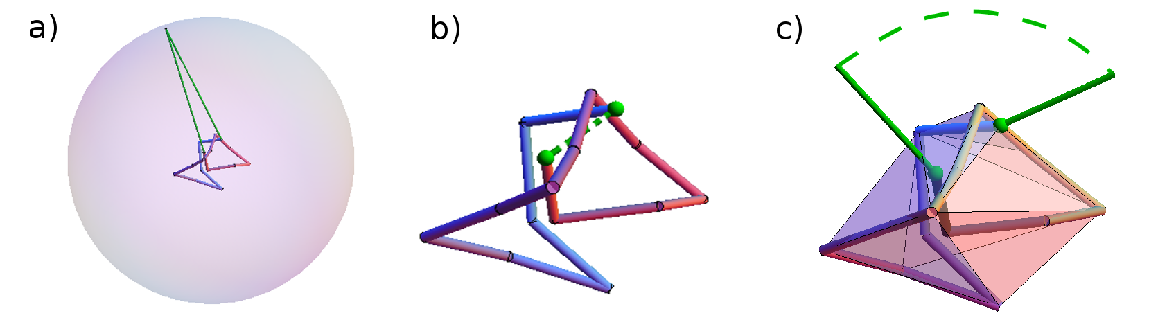
Figure 1: Sketched examples of the closure schemes used in this work: (a) Stochastic closure at infinity, (b) direct bridging, (c) minimally interfering closure.

As anticipated in the introduction, one needs to introduce a well-defined procedure to close, or circularize, various subportions of the ring under consideration so as to properly establish their topological state.

Several viable closure schemes are considered, including some that have been introduced and applied before.

Before describing the various closure schemes we clarify the notation that will be used from now on. For a given ring, $\Gamma=\{\vec{r}_{1},\vec{r}_{2},\ldots,\vec{r}_{N},\vec{r}_{N+1}=\vec{r}_{1}\}$, we denote by $\Gamma_{ij}=\{\vec{r}_{i},\ldots,\vec{r}_{j}\}$ the arc comprising all edges from vertex $i$ to vertex $j$ (including the endpoints $i$ and $j$). The orientation of $\Gamma_{ij}$ follows the one given by the increasing numbering of the nodes on the full ring.

The three following schemes are used to close a given arc $\Gamma_{ij}$:

1. Direct bridging. The two arc ends, $i$ and $j$ are directly joined by a straight segment (Fig. 1 (b)) JansevanRensburg:1992:J-Phys-A .

2. Stochastic closure at infinity. This scheme, introduced in ref. Millett_2005_Macromol consists in closing $\Gamma_{ij}$ by connecting its ends to a point picked randomly on a sphere centred at the centre of mass of the arc and with radius much larger than the radius of gyration of $\Gamma_{ij}$, see Fig. 1 (a). The random closure procedure is repeated a large number of times (1000 in this study), and the topological state with the largest statistical weight is identified. If this weight exceeds a preassigned threshold, $q$, then the dominant topological state is taken as the topological state of the arc $\Gamma_{ij}$. Otherwise, the topology of $\Gamma_{ij}$ is considered ambiguous and is left undetermined. In this study we consider two different threshold values: $q=50\%$ and $q=90\%$.

3. minimally-interfering closure The amount of entanglement introduced by closing the arc $\Gamma_{ij}$ is intuitively expected to grow with the distance spanned by the added closing segments inside the convex hull of $\Gamma_{ij}$. In order to minimize such “interference” we consider two alternative closures. In the first closure, the two endpoints of $\Gamma_{ij}$ are prolonged through their nearest points on the convex hull (computed with the QuickHull algorithm Barber_et_Al_quickhull_1996 ) and connected with an arc at infinity. The sum of the distance of each of the two endpoints from the closest point on the convex hull, $d^{out}_{ij}$ is taken as the measure of the associated. This quantity is compared to the geometrical distance of the two points, $d^{in}_{ij}$, which is a measure of the interference associated to the direct bridging closure. The minimally-interfering closure is picked by comparing $d^{out}_{ij}$ and $d^{in}_{ij}$. If $d^{in}_{ij}>d^{out}_{ij}$ then the enpoints are joined using their prolongations to infinity (Fig. 1(c)), otherwise they are directly bridged (Fig. 1(b)).

A pleasing feature of the minimally-interfering closure is that when the boundary of the convex hull of an arc contains the arc termini, then it is straigthforward to check whether the hull and the arc realize a ball-pair. For this check one should ascertain that the convex hull is not pierced by the edges of the rest of the ring. In addition, the closure appears appropriate for deeply buried termini too which, as intuitively expected, will be directly joined.

II.3 Knot localization schemes

A few different procedures have been proposed so far to localize the shortest knotted portion of a ring with non-trivial topology Katrich:2000:PRE ; Marcone:2005:J-Phys-A ; Mansfield2010 . They can be divided into two main categories depending on the strategy used to search for the shortest knotted portion of a ring.

To illustrate the two methods, let us consider a trefoil knot in a ring of $N$ vertices.

The first procedure involves a bottom-up search for the knot. The purpose is to identify the shortest portion of the ring that has the same topology of the whole ring. One starts by considering all portions of the ring (arcs) with a small contour length, $l$, (small means no larger than the length required to tie a trefoil knot). If, after closure, none of the arcs is found to be trefoil knotted, then $l$ is increased by one and the search for a trefoil-knotted arc starts again. Clearly the search stops when one arc of the current contour length, $l$, is found to be trefoil knotted. We shall refer to this arc as the shortest knotted arc. It is important to stress that the returned shortest knotted arc may correspond to an ephemeral knot. These are arcs with non-trivial topology that are contained in longer arcs with a different topology (which, in turn, can be contained inside arcs with different topology etc) Millett:2010:JKTR .

To avoid detecting ephemeral knots one can resort to a second method, that involves a top-down search. In this case one looks for the shortest knotted portion of the ring that (i) cannot be further shortened without losing the knot and (ii) can be extended continuosly to encompass the whole ring. To do so, one begins by setting $l=1$ and considers all arcs of length $N-l$ and discards those that are not trefoil-knotted. Then $l$ is increased by one unit and, inside the survived arcs, one looks for trefoil-knotted arcs of length $N-l$. Those that are not trefoil-knotted are discarded and the procedure is repeated until at a certain value of $l=\bar{l}$ no trefoil-knotted arc is found. The trefoil-knotted arc (or arcs in case of degeneracy) that survided at the previous iteration step (the one(s) with length $N-(\bar{l}+1)$) provides the desired ring portion accommodating the knot. We shall refer to such arc(s) as the shortest continuously-knotted portion of the ring, or shortest C-knotted portion for brevity.

The knotted portions identified by the two procedures are not necessarily the same, as illustrated in Fig. 2. From the two definitions it follows that the length of the shortest C-knotted arc cannot be smaller than that of the shortest knotted arc.

Both methods are applied and compared in this study, but with one important addition with respect to the procedure described above. The modification follows the observation that a satisfactory location of the trefoil knot in a specific arc, $\Gamma_{ij}$, of the ring should be accompanied by the condition that the complementary arc, $\Gamma_{ji}$, is unknotted. Therefore the test for “trefoil-knottedness” in the previous schemes, consists in the stringent requirement that upon closure $\Gamma_{ij}$ is trefoil knotted and its complementary arc, $\Gamma_{ji}$ is unknotted.

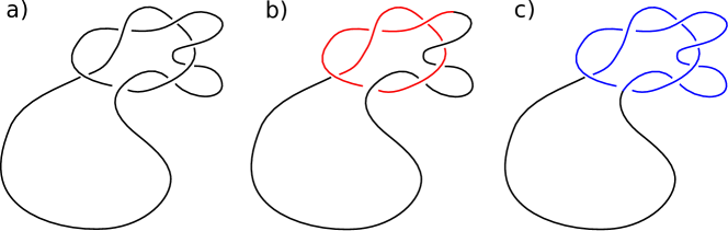
Figure 2: An example of how a bottom-up (b) and a top-down search (c) on the trefoil knotted arc shown in (a) give rise respectively to the shortest knotted arc (red curve in (b)) and to and shortest C-knotted arc (blue curve in (c)).

III Results

III.1 Knot matrices

The closure schemes described in section II.2 were applied to all arcs of the three rings of $N=100$ edges shown in Fig. 4, 5 and 6.

For each ring we considered all possible $N(N-1)$ oriented arcs $\Gamma_{ij}$ with $i\neq j$. After circularization, the topological state of each arcs was established by using the KNOTFIND routine implemented in the KNOTSCAPE package Knotscape . The KNOTFIND routine efficiently simplifies the diagrammatic representation of a knot and compares it against a look-up table of diagrams of prime knots with less than 17 minimal crossings. When a positive match is found, the topological state of the ring is unambiguously established. If no match is found (due to genuine excessive complexity of the knot or to insufficient classification) the topological state is regarded as undetermined.

The topological states of all arcs $\Gamma_{ij}$ are conveniently reported as the $(i,j)$ element of an $N\times N$ “knot matrix”. The knot matrix entries, which take on discrete values reflecting the variety of knots trapped in the arcs, are conveniently conveyed in color-coded graphical representations, see Fig. 3. The graphical representation adopted here follows the indexing convention first introduced by Yeates and coworkers to highlight the presence of slipknots in naturally-occurring proteins King_et_al_2007_J_Mol_Biol . By convention the diagonal of the matrix is taken to correspond to the whole ring.

As illustrated in Fig.3 by analysing the matrix it is possible to recover a wealth of information about the interplay of the geometrical and topological entanglement of the ring. In particular it is possible to identify the shortest knotted arc and the shortest C-knotted arc as well as identifying ephemeral knots Millett:2010:JKTR .

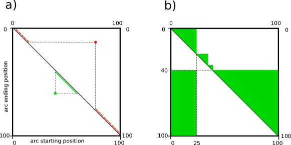
Figure 3: A ring of $N$ edges is associated to $N\times N$ knot matrix. Unlike the case of open chains  King_et_al_2007_J_Mol_Biol the matrix is periodic. To each entry, $i,j$ of the matrix is associated an oriented arc $\Gamma_{i,j}$ of the ring going from $\vec{r}_{i}$ to $\vec{r}_{j}$. This is illustrated in panel (a), where the arcs associated to the two different marked entries are highlighted on the matrix diagonal. The topological state of an arc is encoded by the color of the corresponding matrix entry. In the example shown in panel b white is used for the unknot and green for the trefoil knot. The shortest knotted arc of a knotted ring is the shortest subarc having the same topology of the ring while its complementary arc stays unknotted. For this ring it corresponds to the arc $\Gamma_{25,40}$ which coincides with the shortest continuously-knotted arc too (see Methods for the definition).

Knot matrices have been computed for all the closure schemes presented in (II.2). Their visual inspection and interpretation according to Fig. 3 readily conveys the salient differences across the closure methods in establishing the degree of entanglement of various ring subportions.

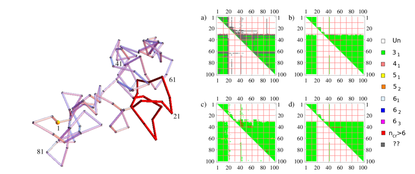
Figure 4: Leftmost panel: spatially-unconstrained trefoil-knotted ring of $N=100$ edges. The indices (numbering) of subset of vertices are shown explicitly; the first vertex is highlighted with a yellow sphere. Other panels: knot matrices of the ring obtained by using $4$ different closure schemes: stochastic closure at infinity with threshold (a) $q=90$% and (b) $q=50$%, (c) direct bridging and (d) minimally-interfering closure. Different topologies are color-coded according to the legend on the right. The knotted portion dentified by using the minimally-interfering closure is highlighted in red. In this case the shortest knotted and C-knotted arcs coincide.

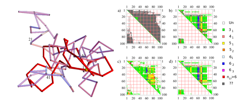
Figure 5: Mildly-confined trefoil-knotted ring of $N=100$ edges (leftmost panel ) and associated knot matrices displayed and coloured as in Fig. 4. The shortest knotted arc computed with the minimally-interfering closure is highlighted in red. The shortest C-knotted arc computed with the same closure is shown with red interior. Note that the shortest continuously-knotted arc, $\Gamma_{51,16}$ contains the shortest knotted arc, $\Gamma_{87,15}$

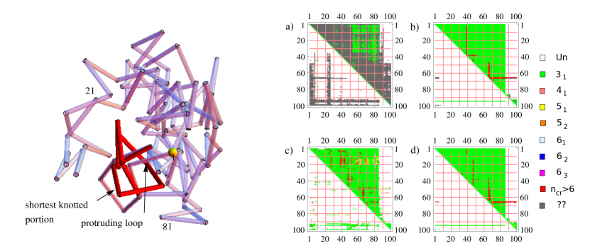
Figure 6: Strongly confined trefoil ring of $N=100$ edges ( leftmost panel ) and associated knot matrices displayed and coloured as in Fig. 4. The shortest knotted arc computed by using the minimally-interfering closure (highlighted in red) is an ephemeral knot with a protruding loop (shown with red interior) which is contained inside a larger trefoil-knotted arc. The union of the shortest knotted arc and the protruding loop coincides with the shortest continuously-knotted arc.

III.2 Unconstrained case

We start by discussing the knot matrices for the unconstrained ring in Fig. 4. From an overall visual inspection, the various knot matrices appear largely consistent and the topologies of most arcs correspond to either unknots or trefoil knots.

Yet, as it is visible in panels (b), (c) and (d), a limited occurrence of knots with more than $6$ minimal crossings is found for arcs of various lengths that either start or end at vertex number $41$. For example the arc $\Gamma_{41,39}$ is seen as a knot with more than 6 minimal crossings by all the closing schemes. These instances are manifestly ephemeral knots because their topological state differs from the global one of the ring, which is the trefoil.

Note that for this ring, all schemes are consistent. This fact is compatible with the finding of ref. Millett_2005_Macromol that, for unconstrained rings, the dominant knot type found with the stochastic closures with threshold $q=50\%$ is usually the same one obtained with the direct closure scheme.

Regarding the robustness of the closure scheme in terms of the threshold, $q$, we report that for $q=90$% about $15\%$ of the entries are marked as undetermined knots (grey color). These undetermined arcs represent cases where the details of the closure scheme can likely yield different results. It is interesting to observe that across panels (b), (c) and (d) most arcs whose topology is not the trefoil or the unknot, correspond to undetermined entries in panel (a).

It should also be noted that the direct bridging closure scheme introduces “jagged” boundaries separating the trefoil and unknotted regions. Sharper boundaries are instead found for the stochastic closure ($q=50$%) and the minimally-interfering closure.

III.3 Spatially-confined cases

The analysis presented above was repeated for the more compact configuration depicted in Fig. 5.

The increased level of geometrical complexity compared to the unconstrained case is conveyed by the fact that a much larger fraction of the matrix entries ($\sim 45\%$) have an undetermined topological state according to the stochastic closure scheme with the stringent $q=90$% threshold. This is because the geometrical complexity characterizing more compact structures prevents the occurrence of a single highly-dominant knot type.

A related aspect is that the knot matrix obtained with the direct bridging closure, see panel (c), is considerably noisier that the knot matrices obtained with the tolerant ($q=50$%) stochastic closure and the minimally-interfering one, see panels (b) and (d).

Notably, the visual inspection of panels (b) and (d) indicates that the responses of these two methods remain highly compatible notwithstanding the increased geometrical complexity.

All the above considerations hold also for the ring with highest level of compactification shown in Fig. 6.

In summary, at all the three levels of compactness a high consistency is found between the tolerant stochastic closure and the minimally-interfering one. Given the different spirit of these two methods this accord is both pleasing and important because it provides a posteriori confidence that a consensus indication of the topological state of various arcs of a ring can be achieved with these two different closure methods.

It is important to point out that, despite returning consistent results, these two methods are very different in terms of the computational espenditure because the stochastic closure scheme is based on a collection of several (in our case 1000) random closures per arc whereas only two closures per arc are involved in the minimally-interfering scheme. The latter scheme appears therefore to be preferable when one seeks to establish the local level of entanglement over a large ensemble of rings or open chains (as for large-scale surveys for detecting and locating knots in all available structures of globular proteins King_et_al_2007_J_Mol_Biol ; Plos2010 .) The former, however, has the advantage of providing a quantitative control of the statistical weight (and hence the robustness) associated to the dominant knot type for every arc.

III.4 Locating the knot

To locate the trefoil knot within each of the three rings under analysis we processed the associated knot matrices obtained by applying the minimally-interfering closure. We use both the top-down and the bottom-up approaches to locate the knot. The results are described herafter and are practically identical to those obtained by using as input the knot matrices obtained with the tolerant ($q$=50%) stochastic closure.

For the unconstrained knot, the two search methods identify the same arc, see Fig. 6, as the region that accommodates the knot.

This is not the case for the two more compact rings. In particular, for the ring shown in Fig. 5 the shortest knotted arc corresponds to $\Gamma_{87,15}$ (highligthed in red in the figure) while the shortest C-knotted arc corresponds to the much longer arc $\Gamma_{51,16}$ shown with red interior.

Finally, for the most compact ring, the shortest knotted arc is found to be $\Gamma_{86,95}$ while the shortest C-knotted arc is found to be $\Gamma_{86,1}$, see Fig. 6. In this case the comparison between the two knot localization methods reveals a notable hierarchy of ephemeral knots. In fact, while arc $\Gamma_{86,95}$ is trefoil knotted, the longer arcs from $\Gamma_{86,96}$ up to $\Gamma_{86,99}$ are uknotted and still longer arcs, such as $\Gamma_{86,1}$, are trefoil-knotted again.

It therefore appears that the increased geometrical complexity of the rings resulting from the isotropic spatial confinement produces a non-trivial interplay of geometry and topology, which manifests in the sensitive dependence of the knot location on the search strategy that is used. A systematic study of the broader implications of this finding is currently underway.

As a final remark we point out that when dealing with large datasets of rings or suitably closed polymer chains, as in large-scale surveys of knotted proteinsPlos2010 ; Virnaupdb , the calculation of the knot detection and knot localization can be speeded up by an initial simplification of the ring geometry. In principle, such changes could affect the outcome of the knot localization procedure. While a systematic study of this effect is beyond the scope of the present investigation, we report in the Appendix a limited discussion of the matter.

IV Conclusions

The main aim of this work was to investigate the efficiency and reliability of different closure schemes in assigning a topological state to a given subportion of a ring and to characterize the topologically-entangled region of knotted rings when they are subjected to different levels of compactification. The detailed analysis of the local entanglement of the ring described in terms of knot matrices shows that two independent closure schemes yield robust and consistent results at all level of ring compactification: the stochastic closure and the minimally-interfering closure.

The two methods, while providing consistent results, have different advantages. The stochastic closure scheme, in fact, provides a statistical confidence level on the robustness of the dominant topological entanglement associated to each considered arc. This valuable information comes at the cost of performing a large number of statistically independent closures on the arc of interest. The statistical robustness information is not directly available in the minimally-interfering scheme as this requires only two closures. But for this very reason the minimally-interfering method is much faster than the stochastic and yet typically returns the same dominant knot type. Considerations of these aspects can guide the choice of which of the two methods should be adopted in a specific study.

The interplay of geometry and topology in rings with different degree of compactness was finally examined by comparing two different methods for knot localization (involving a bottom-up and top-down search, respectively). The analysis indicates that for spatially unconstrained rings the location of the knot can be performed in a consistent manner by the two methods. Appreciable differences between the methods emerge for the more compact configurations, signalling a non-trivial increase of the geometrical complexity of confined polymer rings.

Appendix A Effect of ring simplification

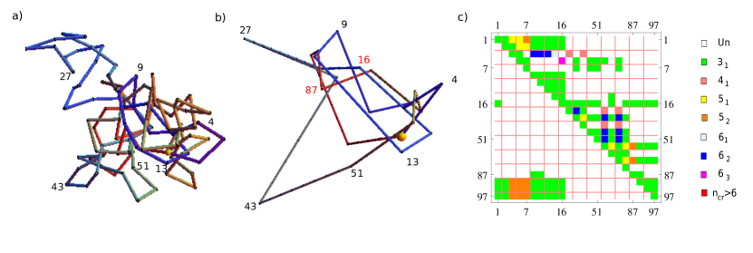
Figure 7: (a) Original and (b) simplified ring after the rectification procedure. The original index (numbering) of a subset of vertices is shown explicitly. The first vertex is highlighted with a yellow sphere. The knot matrix of the simplified ring is shown in panel (c). The full knot matrix of the original ring is shown in Fig. 5 panel (d).

In the attempt to reduce the heavy computational cost of locating the knot either in rings or linear chains, several groups have avoided the extensive topological profiling of all arcs of the ring and have instead mapped out the topology of a simplified representation of it Koniaris&Muthukumar:1991b ; Taylor:2000:Nature:10972297 ; Virnau:2005:JACS:127 .

The simplification, or rectification procedure entails the removal of those ring vertices which can be made collinear with their neighbouring pair along the ring through a continuous local deformation (morphing) of the ring that does not lead to any edge crossing. Such rectification operations clearly preserve the topology of the ring and can considerably reduce the number of ring vertices, and hence the linear size of the knot matrices.

Here we discuss the effect of rectification procedure on the two knot localization schemes introduced in II.3.

In order to ensure the most uniform level of simplification, we subjected each ring on $N$ edges to several simplification rounds. At each stage of the procedure we disallow the removal of ring vertices that would introduce a gap larger than $s$ in the original index of consecutive surviving beads. Because of the ring periodic boundaring conditions, we employ the modulus operation on $s$. By starting with $s=2$ we carry out $N$ statistically-independent attempts at bead removal (sweep). Then $s$ is increased by one and another sweep of vertices elimination is attempted. The procedure is carried on until no vertex can be further removed within a sweep. Notice that more beads might be removed by allowing $s$ to increase even further, but these more aggressive rectifications are not considered here.

Reducing the number of beads of the ring has two distinct effects. First, the linear dimensions of the knot matrix are reduced. Second, the topological entanglement of the remaining subportions might be different from the one measured for the corresponding subportions of the original ring. Regarding the first aspect we recall that we establish the entanglement trapped in the arcs of the surviving nodes by closing the arcs with the same ends on the original, unsimplified ring. As a consequence the knot matrix of the simplified ring is a subset of the original full knot matrix, obtained by restricting to the rows and columns pertaining to the surviving ring vertices. This procedure is illustrated in Fig 7.

Notice that because the simplified knot matrix is a subset of the original knot matrix, then the length of the shortest knotted arc measured on the simplified ring can not be smaller than the length of the shortest knotted arc measured on the unsimplified ring. On the other hand no such reasoning can be made for the shortest C-knotted arc.

The rectification procedure clearly brings about a simplification of the geometrical complexity of the ring. As a consequence, the difference between the shortest knotted arc and shortest C-knotted arc will likely decrease after rectification but it will not be obliterated for sufficiently entangled rings. This is illustrated by the rectification of the ring with intermediate compactness, whose simplified knot matrix is shown in Fig. 7. The shortest knotted arc on the simplified ring goes from node 87 to node 16. The inspection of the matrix reveals that from the point $(87,16)$, corresponding to the shortest knotted arc $\Gamma_{87,16}$, one cannot find a connected path through points corresponding to longer and longer trefoil-knotted arcs (even disregarding the unknottednedd requirement on the complementary arcs) that reach out to the whole ring. This clarifies that $\Gamma_{87,16}$ does not correspond to the shortest C-knotted arc, and hence the two methods for knot detection do necessarily not coincide even after simplification.

References

- (1) J. des Cloizeaux J. de Physique Lett. 42 (1981), L433.
- (2) N. T. Moore and R. C. Lua and A. Y. Grosberg Proc. Natl. Acad. Sci. USA 101 (2004), 13431.
- (3) A. Stasiak, V. Katritch, J. Bednar, D. Michoud and J. Dubochet Nature 384 (1996), 122.
- (4) C. Weber, A. Stasiak, P. De Los Rios and G. Dietler Biophys. J. 90 (2006), 3100.
- (5) E. Orlandini, A. L. Stella and C. Vanderzande To appear in Phys. Rev. E (2010).
- (6) A. M. Saitta, P. D. Soper, E. Wasserman and M. L. Klein Nature 399 (1999), 46.
- (7) D. Marenduzzo, E. Orlandini, A. Stasiak, D.W. Sumners, L. Tubiana and C. Micheletti Proc Natl Acad Sci U S A 106, (2009), 22269.
- (8) E. Orlandini, A. L. Stella and C. Vanderzande Phys. Biol. 6 (2009), 025012.
- (9) B. Marcone, E. Orlandini, A. L. Stella and F. Zonta Phys. Rev. E 75 (2007), 041105.
- (10) E. Orlandini and S. G. Whittington Rev. Mod. Phys. 79 (2007), 611.
- (11) K. Millett, A. Dobay and A. Stasiak Macromol. 38 (2005), 601.
- (12) J. P. J. Michels and F. W. Wiegel Proc. R. Soc. Lond. A403 (1986), 269.
- (13) C. Micheletti, D. Marenduzzo, E. Orlandini and D. W. Sumners J. Chem. Phys. 124 (2006), 64903.
- (14) C. Micheletti, D. Marenduzzo, E. Orlandini and D. W. Sumners Biophys. J. 95 (2008), 3591.
- (15) M. Baiesi, E. Orlandini and S. G. Whittington J. Chem. Phys. 131 (2009), 154902.
- (16) E. Panagiotou, K. C. Millett and S. Lambropoulou J. Phys. A: Math. Theor. 43 (2010), 045208.
- (17) V. Katrich, W.K. Olson, A. Vologodskii, J. Dubochet and A. Stasiak Phys. Rev. E 61 (2000), 5545.
- (18) B. Marcone, E. Orlandini, A. L. Stella and F. Zonta J. Phys. A Math. Gen. 38 (2005), L15.
- (19) M.L. Mansfield and J.F. Douglas J. Chem. Phys. 133 (2010), 044903.
- (20) J. Arsuaga, M. Vázquez, P. McGuirk, S. Trigueros, D. W. Sumners, J. Roca Proc Natl Acad Sci U S A 102, (2006), 9165.
- (21) D. Marenduzzo, C. Micheletti and E. Orlandini J. Phys. Condens. Matter 22 (2010), 283102.
- (22) C. Micheletti, D. Marenduzzo and E. Orlandini Physics Reports (2011), in press.
- (23) E. J. Janse van Rensburg, D. W. Sumners, E. Wasserman and S. G. Whittington J. Phys. A: Math. Gen. 25 (1992), 6557.
-
(24)
C. Bradford Barber, D. P. Dobkin, H. Huhdanpaa
J. ACM Trans. Math. Softw. 22 (1996), 469.
http://www.qhull.org - (25) K. Millett J. Knot Theory its Ramif. 19 (2010), 601.
-
(26)
J. Hoste and M. Thistlethwaite
KnotScape 101
Software Package: www.math.utk.edu/morwen/knotscape.html. - (27) N. P. King, E. O. Yeates and T. O. Yeates J. Mol. Biol. 12 (2007), 153.
- (28) R. Potestio, C. Micheletti and H. Orland H PLoS Comput. Biol. 6 (2010), e1000864; doi:10.1371/journal.pcbi.1000864
- (29) P. Virnau, L.A Mirny and M. Kardar PLoS Comput. Biol. 2 (2006), e122; doi: 10.1371/journal.pcbi.0020122.
- (30) K. Koniaris, M. Muthukumar J. Chem. Phys. 95 (1991), 2873.
- (31) W. R. Taylor Nature 406 (2000), 916.
- (32) P. Virnau, Y. Kantor and M. Kardar J. Am. Chem. Soc. 127 (2005), 15102.