Theory of excitons in cubic III-V semiconductor GaAs, InAs and GaN quantum dots: fine structure and spin relaxation

Abstract

Exciton fine structures in cubic III-V semiconductor GaAs, InAs and GaN quantum dots are investigated systematically and the exciton spin relaxation in GaN quantum dots is calculated by first setting up the effective exciton Hamiltonian. The electron-hole exchange interaction Hamiltonian, which consists of the long- and short-range parts, is derived within the effective-mass approximation by taking into account the conduction, heavy- and light-hole bands, and especially the split-off band. The scheme applied in this paper allows the description of excitons in both the strong and weak confinement regimes. The importance of treating the direct electron-hole Coulomb interaction unperturbatively is demonstrated. We show in our calculation that the light-hole and split-off bands are negligible when considering the exciton fine structure, even for GaN quantum dots, and the short-range exchange interaction is irrelevant when considering the optically active doublet splitting. We point out that the long-range exchange interaction, which is neglected in many previous works, contributes to the energy splitting between the bright and dark states, together with the short-range exchange interaction. Strong dependence of the optically active doublet splitting on the anisotropy of dot shape is reported. Large doublet splittings up to 600 $\mu$eV, and even up to several meV for small dot size with large anisotropy, are shown in GaN quantum dots. The spin relaxation between the lowest two optically active exciton states in GaN quantum dots is calculated, showing a strong dependence on the dot anisotropy. Long exciton spin relaxation time is reported in GaN quantum dots. These findings are in good agreement with the experimental results.

I INTRODUCTION

Semiconductor quantum dots (QDs) have attracted intense interest due to the high potential to work as basic device units for photonics, spintronics, quantum communication and computation.Barenco ; Biolatti ; Lovett ; Boyle ; Loss ; Hanson ; Klauser One of the applications is to use QDs as emitter of single photonMichler ; Yuan ; Shields ; Santori2 and entangled photon pairsBenson ; Stev ; Avron ; Akopian ; Greilich ; Hafenbrak ; Stevenson via the combination of exciton and biexciton. Explicitly, for a symmetric QD, the decay of the bright (optically active) exciton statesIvchenko5 with total angular momentum projections $J_{z}=\pm 1$ can emit $\sigma^{\pm}$ circularly polarized photons, while that of the biexciton states through two intermediate degenerate bright exciton states can generate two entangled photons.Benson ; Mohan The asymmetry of QDs lifts the degeneracy of the two bright exciton states and mixes them into two states that generate linearly polarized photons with orthogonal polarizations during the decay.Akopian ; Greilich ; Santori ; Gammon ; Besombes This is even crucial when considering the biexciton decay as the splitting of the intermediate exciton states makes the two channels distinguishable and hence destroys the entanglement.Avron ; Santori ; Ulrich ; Stevenson Moreover, the dark (optically forbidden) exciton states which lie slightly below the bright onesIvchenko5 are considered promising candidates for spin qubits due to their long lifetimes when confined in QDs.Imam ; Johansen They also play a key role for the Bose-Einstein condensation in semiconductors.Combescot

The splitting between the bright and dark exciton states (denoted as the BD exchange splitting hereafter)Nirmal ; Bayer2 and that between the bright exciton states (denoted as the doublet splitting hereafter)Seguin ; Young ; Stevenson2 ; Dovrat ; Sugisaki ; Seguin2 are mainly controlled by the electron-hole (e-h) exchange interaction together with the dot size and asymmetry.Bayer1 ; Taka2 ; Zunger2 ; Kindel ; Young ; Besombes So a detailed understanding of the e-h exchange interaction and the resulting exciton fine structure in QDs is of fundamental importance for both theoretical and application purposes.

The e-h exchange interaction has been investigated ever since the 1960s. It can be decomposed into long- and short-range parts in the real spaceKnox ; Bir1 ; Bir2 or the analytical and nonanalytical parts in the ${\bf k}$ space.Denisov ; Ivchenko2 There is a close correspondence between them which can be found in Ref. Cho1, , and sometimes no difference is made between these two approaches.Ivchenko1

Early investigations on the e-h exchange interaction mainly focus on the bulk system.Heller ; Denisov ; Onodera ; Abe ; Elliott ; Rossler ; Bonneville ; Suga ; Andreani2 It is well known that, when considering the exciton states in semiconductors by taking into account the conduction band $\Gamma_{6}^{c}$ and the valence band $\Gamma_{8}^{v}$, the short-range (SR) exchange interaction splits the eightfold-degenerate exciton state into a triplet bright state and a quintuplet dark state with the splitting energy between them, the so-called exchange energy.Bonneville ; Suga The long-range (LR) exchange interaction further splits the triplet into a longitudinal and two transverse modes, the energy difference of which is denoted as the longitudinal-transverse splitting.Bonneville ; Suga ; Andreani2 The e-h exchange interaction, as well as the direct Coulomb interaction, is greatly enhanced by the quantum confinements in low-dimensional semiconductor structures because of the increased spatial overlap between the electron and hole wave functions. Reexamination of the e-h exchange interaction in low-dimensional structures was intrigued in both experimentalBauer ; Kesteren ; Norris ; Chamarro ; Amand and theoreticalJorda ; Ivchenko5 ; Chen ; Andreani ; Maialle ; Taka1 ; Taka2 ; Efros ; Horo ; Kalt1 ways. Most of the theoretical works were carried out within the framework of the envelope-function approximation together with the effective-mass approximation.Chen ; Andreani ; Maialle ; Taka1 ; Taka2 ; Efros ; Horo ; Kalt1 In general, due to the different effective masses of the heavy, light and split-off holes, the heavy-, light- and split-off-hole exciton statesnote0 are energetically split when a quantum confinement is applied. For common cubic III-V semiconductors, the heavy-hole exciton which energetically lies the lowest is of most physical interest and is hence mostly investigated.Chen ; Bauer ; Andreani ; Maialle ; Kesteren ; Kalt1 ; Kalt2 ; Kalt3 ; Ivchenko3 ; Kada The heavy-hole exciton quartet, which is characterized by the total angular momentum projections $J_{z}=\pm 1$, $\pm 2$, is split into bright and dark exciton states with $J_{z}=\pm 1$ and $J_{z}=\pm 2$, respectively, by the e-h exchange interaction and the bright exciton states $|\pm 1\rangle$ are further split under anisotropic confinement potential. Chen et al.Chen calculated the exchange energy and the BD exchange splitting in GaAs/${\rm Ga}_{1-x}{\rm Al}_{x}{\rm As}$ quantum wells (QWs) and evidenced the enhancement of the exchange effect with decreasing well width. Their work was based on the approximation of decoupled heavy- and light-hole subbands. Andreani and Bassani investigated the ${\bf k}$ dependence of the e-h exchange interaction in QW systems.Andreani In Ref. Maialle, the exciton spin dynamics in GaAs QWs was studied with e-h exchange interaction as an effective spin-flip mechanism, where the matrix elements of the LR exchange interaction were calculated by using the simple heavy-hole exciton ground states while those of the SR exchange interaction were obtained by taking into account the mixing of heavy- and light-hole bands. Takagahara performed systematic studies of exciton states in QDs in Ref. Taka1, . The exciton binding energy and the LR and SR exchange interactions were investigated using wave functions calculated by the variational method. The subband mixing induced by the direct Coulomb interaction was pointed out to be important. In a later work for GaAs QDs,Taka2 Takagahara derived an eight-band exciton Hamiltonian. The LR exchange interaction, which was attributed to dipole-dipole interaction, was emphasized to be much more important than the SR exchange interaction when concerning the exciton doublet fine structure. The contradiction of the calculated scaling law of the doublet splitting energy to the theoretical prediction was reported (also in Ref. Kada, ). Whereas in the latter works by Tsitsishvili et al.Kalt1 ; Kalt2 the exciton spin relaxation in single asymmetrical QD was studied by taking into account only the SR exchange interaction. Efros et al.Efros and Horodyská et al. in their very recent workHoro investigated the band-edge exciton states in spherical QDs by including only the SR exchange interaction. But actually, as will be shown in this paper, the LR exchange interaction contributes to the splitting between bright and dark exciton states even in isotropic QDs where the doublet splitting energy vanishes. Its contribution to the BD exchange splitting can be comparable with that from the SR exchange interaction. Moreover, although the direct Coulomb interaction is believed to lead to poor convergence if treated perturbatively when the exciton system is in the weak confinement regime, in a very recent work by Kadantsev and Hawrylak,Kada the exciton fine structure in GaAs QDs was still studied by taking the direct Coulomb interaction as perturbation.

Thus, even though a lot of works have been done on the e-h exchange interaction induced exciton properties, obvious confusions are still seen in the literature, even for the most investigated In_1-xGa_xAs nanostructures. The significance of valence-band coupling to the exciton fine structure needs to be evaluated. The relative importance of the LR and SR exchange interactions to the doublet splitting needs more elaboration, and that to the BD exchange splitting needs to be clarified. Furthermore, the size scaling of the e-h exchange interaction and the influence of the direct Coulomb interaction on the exciton fine structure have to be examined and stressed.

Works discussed above mainly concern III-V semiconductor nanostructures based on In_1-xGa_xAs the split-off band of which is far away from the heavy- and light-hole bands.Vurga So the split-off band is always neglected when studying exciton fine structure. However, for cubic GaN, whose spin-orbit splitting is small compared to the wide band gap,Vurga no theoretical work has been performed to investigate exciton fine structure so far, nor does the explicit expression of e-h exchange Hamiltonian with the effect of split-off band exists in the literature. It has been proved that in bulk GaN, the split-off band is important when considering the spin-orbit coupling.Fu Whether it is still the case when studying the e-h exchange interaction in GaN QDs needs to be examined.

The exciton spin relaxation is another important subject that strongly affects the quality of applications in information storage and processing based on exciton states in QDs.Kalt1 ; Kolli ; Smith ; Astakhov Motivated by recent experimental study of exciton spin orientation in cubic GaN/AlN QDs,Marie we investigate the behavior of the LR and SR exchange interactions in cubic III-V semiconductor QDs, taking into account all heavy-hole, light-hole and split-off bands. The spin relaxation between the lowest two bright exciton states in single GaN QD is studied after that.

In this paper, in order to explicitly include the effect of the split-off band on the exciton fine structure in cubic GaN, GaAs and InAs QDs, the bulk e-h exchange Hamiltonian of both LR and SR parts is first derived in the $12\times 12$ matrix representation. The derivation is carried out within the framework of the effective-mass approximation.Winkler For systems strongly confined in one direction, e.g., the QD system with small dot height considered in this paper, we are able to apply the Löwdin partitioning methodWinkler ; Lowdin ; Luttinger2 to approximately diagonalize the modified $6\times 6$ Luttinger Hamiltonian (specified in Sec. II) for holes to obtain a new “heavy-hole” band, which is an admixture of the heavy-hole, light-hole and split-off bands. In this way, $4\times 4$ matrix representations of the exciton exchange Hamiltonian are constructed by taking the conduction band and the new “heavy-hole” band with the effect of valence-band mixing included. We then apply the effective Hamiltonian obtained to investigate the exciton fine structures in cubic III-V semiconductor QDs. The doublet splitting energy and the BD exchange splitting are calculated and the relative importance of the LR and SR exchange interactions as well as that of the heavy-hole, light-hole and split-off bands are discussed. The size scalings of the doublet splitting energy and the BD exchange splitting contributed by the LR and the SR exchange interactions are analyzed and explained by the scaling rules established.

Due to the fact that the values of the exciton Bohr radius in bulk GaAs, InAs and GaN are 14.9 nm, 51.6 nm and 4.8 nm,Ekardt respectively, which are comparable or even smaller than the average diameter of the QDs in this paper (given in Sec. III), chosen according to the experiments,Marie ; Bayer1 ; Bayer2 ; Raymond the direct Coulomb interaction is too large to be treated perturbatively. We solve the Schrödinger equation by taking the direct Coulomb interaction and the confinement in an equal footing. The calculated exciton binding energies are found to be considerably large, markedly enhanced by the confinement. This contradicts the results in the latest work by Kadantsev and HawrylakKada and further demonstrates the importance to treat the direct Coulomb interaction unperturbatively. The importance of the direct Coulomb interaction to the exciton fine structure is demonstrated. Finally, the exciton spin relaxation rates in single GaN QDs are calculated and long spin relaxation time is obtained. Our results are in agreement with experiments.Bayer1 ; Seguin ; Marie

This paper is organized as follows: In Sec. II, we set up our model and lay out the formalism. Matrix representations of LR and SR exchange interactions are derived first in bulk and then in QW. Size-scaling rules are established and exciton spin relaxation assisted by the acoustic phonons are introduced after that. The numerical scheme is laid out at the end of this section. In Sec. III, we show our numerical results of exciton fine structures in GaAs, InAs and GaN QDs. Explicit properties of the LR and SR exchange interactions contributing to the doublet splitting energy and BD exchange splitting are discussed in detail. In Sec. IV, the exciton spin relaxation in single GaN QD is investigated. We conclude in Sec. V.

II MODEL AND FORMALISM

We formulate the theory of excitons in cubic III-V semiconductors by taking into account the conduction band $\Gamma_{6}^{c}$ and the valence bands $\Gamma_{8}^{v}$ and $\Gamma_{7}^{v}$. The effective representations of the exciton Hamiltonian for the LR and SR exchange interactions are derived first in bulk and then in QW. The size-scaling rules of the e-h exchange interaction are established after that. We then introduce the exciton spin relaxation due to the electron/hole–acoustic-phonon scattering. The numerical scheme is laid out at the end of this section.

II.1 e-h exchange interaction

II.1.1 e-h exchange interaction in bulk

We start our investigation on the e-h exchange interaction from a general description of direct Wannier-Mott excitons in bulk system within the framework of effective-mass approximation. The exciton wave function can be written in the formBir1 ; Bir2

$$\Psi({\bf r}_{1},{\bf r}_{2})=\sum_{mn}\big{[}F_{mn}({\bf r}_{1},{\bf r}_{2})\psi_{m{\bf k}_{0}}({\bf r}_{1})\tilde{\psi}_{n{\bf k}_{0}}({\bf r}_{2})$$

$$\mbox{}-F_{mn}({\bf r}_{2},{\bf r}_{1})\psi_{m{\bf k}_{0}}({\bf r}_{2})\tilde{\psi}_{n{\bf k}_{0}}({\bf r}_{1})\big{]},$$ (1)

where $\psi_{m{\bf k}_{0}}({\bf r})$ is the conduction-band Bloch function and $\tilde{\psi}_{n{\bf k}_{0}}({\bf r})$ is the Bloch function for the hole which is the time reversal of the Bloch function of the missing electron.Bir1 ; Bir2 As for cubic III-V semiconductors, we are interested in excitons at the band edge, i.e., the $\Gamma$ point with ${\bf k}_{0}=0$. $m$ ($n$) is the index for the electron (hole) band under consideration, including the spin degree of freedom. $F_{mn}({\bf r}_{1},{\bf r}_{2})$ is the envelope function with $F_{mn}({\bf r}_{1},{\bf r}_{2})=-F_{nm}({\bf r}_{2},{\bf r}_{1})$. This makes the exciton wave function antisymmetric.

The eigen equation for the envelope function $F_{mn}$ is given byBir1 ; Bir2

$$\sum_{mn}\int d{\bf r}_{1}d{\bf r}_{2}H^{\rm eh}_{m^{\prime}n^{\prime}\atop mn}\left({\bf r}^{\prime}_{1}\ {\bf r}^{\prime}_{2}\atop{\bf r}_{1}\ {\bf r}_{2}\right)F_{mn}({\bf r}_{1},{\bf r}_{2})$$

$$\ \ \ \ \ \ \ =EF_{m^{\prime}n^{\prime}}({\bf r}^{\prime}_{1},{\bf r}^{\prime}_{2}).$$ (2)

The explicit form of $H^{\rm eh}_{m^{\prime}n^{\prime}\atop mn}\left({\bf r}^{\prime}_{1}\ {\bf r}^{\prime}_{2}\atop{\bf r}_{1}\ {\bf r}_{2}\right)$ is given in Appendix A.

Now we proceed to a more detailed derivation of the matrix representations of the exchange interaction for cubic III-V semiconductors, such as GaAs, InAs and GaN, by taking into account the conduction band $\Gamma_{6}^{c}$, the heavy-hole and light-hole bands $\Gamma_{8}^{v}$ and the split-off band $\Gamma_{7}^{v}$. The Bloch functions for these bands and the time reversal of those for the valence bands are given in Appendix B.note1 We further denote the conduction band Bloch functions as

$$|c_{1}\rangle=|\frac{1}{2},\frac{1}{2}\rangle_{c},\ \ \ \ |c_{2}\rangle=|\frac{1}{2},-\frac{1}{2}\rangle_{c}.$$ (3)

and the hole Bloch functions as:

$$|v_{1}\rangle=|\frac{3}{2},+\frac{3}{2}\rangle_{h},\ |v_{2}\rangle=|\frac{3}{2},+\frac{1}{2}\rangle_{h},\ |v_{3}\rangle=|\frac{3}{2},-\frac{1}{2}\rangle_{h},$$ (4)

$$|v_{4}\rangle=|\frac{3}{2},-\frac{3}{2}\rangle_{h},\ |v_{5}\rangle=|\frac{1}{2},+\frac{1}{2}\rangle_{h},\ |v_{6}\rangle=|\frac{1}{2},-\frac{1}{2}\rangle_{h}.$$ (5)

We perform the Fourier expansion as $U({\bf r})=\frac{1}{8\pi^{3}}\int d{\bf q}U_{q}e^{i{\bf q}\cdot{\bf r}}$ where $U_{q}=\frac{e^{2}}{\varepsilon_{0}\kappa q^{2}}$, and then the term of LR exchange Hamiltonian in Eq. (85) transforms into the form

$$H^{{\rm LR}}_{m^{\prime}n^{\prime}\atop mn}\left({\bf r}^{\prime}_{1}\ {\bf r}^{\prime}_{2}\atop{\bf r}_{1}\ {\bf r}_{2}\right)=\frac{1}{8\pi^{3}}\int d{\bf q}U_{q}\Big{(}\sum_{\alpha\beta}Q^{\alpha\beta}_{m^{\prime}\Theta n\atop\Theta n^{\prime}m}q_{\alpha}q_{\beta}\Big{)}$$

$$\ \ \ \ \ \mbox{}\times e^{i{\bf q}\cdot({\bf r}_{1}-{\bf r}^{\prime}_{1})}\delta({\bf r}_{1}-{\bf r}_{2})\delta({\bf r}^{\prime}_{1}-{\bf r}^{\prime}_{2}),$$ (6)

with $\Theta$ being the time reversal operator. We define the band-relevant part of the LR exchange Hamiltonian as $Q_{m^{\prime}n^{\prime}\atop mn}({\bf q})$ with

$$Q_{m^{\prime}n^{\prime}\atop mn}({\bf q})=\sum_{\alpha\beta}Q^{\alpha\beta}_{m^{\prime}\Theta n\atop\Theta n^{\prime}m}q_{\alpha}q_{\beta}.$$ (7)

Then the parity of the Bloch functions enables us to write the matrix representation of $Q_{m^{\prime}n^{\prime}\atop mn}({\bf q})$ in a somewhat simple way. With the basis $|mn\rangle$ taken in the order $|c_{1}v_{1}\rangle,|c_{2}v_{1}\rangle,|c_{1}v_{2}\rangle,|c_{2}v_{2}\rangle,|c_{1}v_{3}\rangle,|c_{2}v_{3}\rangle,|c_{1}v_{4}\rangle,|c_{2}v_{4}\rangle,\\ |c_{1}v_{5}\rangle,|c_{2}v_{5}\rangle,|c_{1}v_{6}\rangle$, $|c_{2}v_{6}\rangle$, $Q_{m^{\prime}n^{\prime}\atop mn}({\bf q})$ takes the form

$$Q_{m^{\prime}n^{\prime}\atop mn}({\bf q})=\left(\begin{array}[]{cccccccccccc}0&0&0&0&0&0&0&0&0&0&0&0\\ &A{K^{2}}&{-\frac{AK^{2}}{\sqrt{3}}}&{-\frac{2AK_{-}q_{z}}{\sqrt{3}}}&{\frac{2AK_{-}q_{z}}{\sqrt{3}}}&{-\frac{AK_{-}^{2}}{\sqrt{3}}}&A{K_{-}^{2}}&0&{{\frac{-BK^{2}}{\sqrt{6}}}}&{{\frac{BK_{-}q_{z}}{\sqrt{6}}}}&{{\frac{BK_{-}q_{z}}{\sqrt{6}}}}&{{\frac{BK_{-}^{2}}{\sqrt{6}}}}\\ &&{\frac{AK^{2}}{3}}&{\frac{2AK_{-}q_{z}}{3}}&{-\frac{2AK_{-}q_{z}}{3}}&{\frac{AK^{2}_{-}}{3}}&{-\frac{AK^{2}_{-}}{\sqrt{3}}}&0&{{\frac{BK^{2}}{3\sqrt{2}}}}&{{-\frac{BK_{-}q_{z}}{3\sqrt{2}}}}&{{-\frac{BK_{-}q_{z}}{3\sqrt{2}}}}&{{-\frac{BK_{-}^{2}}{3\sqrt{2}}}}\\ &&&{\frac{4Aq_{z}^{2}}{3}}&{-\frac{4Aq_{z}^{2}}{3}}&{\frac{2AK_{-}q_{z}}{3}}&{-\frac{2AK_{-}q_{z}}{\sqrt{3}}}&0&{{\frac{\sqrt{2}BK_{+}q_{z}}{3}}}&{{-\frac{\sqrt{2}Bq_{z}^{2}}{3}}}&{{-\frac{\sqrt{2}Bq_{z}^{2}}{3}}}&{{-\frac{\sqrt{2}BK_{-}q_{z}}{3}}}\\ &&&&{\frac{4Aq_{z}^{2}}{3}}&{-\frac{2AK_{-}q_{z}}{3}}&{\frac{2AK_{-}q_{z}}{\sqrt{3}}}&0&{{-\frac{\sqrt{2}BK_{+}q_{z}}{3}}}&{{\frac{\sqrt{2}Bq_{z}^{2}}{3}}}&{{\frac{\sqrt{2}Bq_{z}^{2}}{3}}}&{{\frac{\sqrt{2}BK_{-}q_{z}}{3}}}\\ &&&&&{\frac{AK^{2}}{3}}&{-\frac{AK^{2}}{\sqrt{3}}}&0&{{\frac{BK_{+}^{2}}{3\sqrt{2}}}}&{-{\frac{BK_{+}q_{z}}{3\sqrt{2}}}}&{{-\frac{BK_{+}q_{z}}{3\sqrt{2}}}}&{{-\frac{BK^{2}}{3\sqrt{2}}}}\\ &&&&&&A{K^{2}}&0&{{-\frac{BK_{+}^{2}}{\sqrt{6}}}}&{{\frac{BK_{+}q_{z}}{\sqrt{6}}}}&{{\frac{BK_{+}q_{z}}{\sqrt{6}}}}&{{\frac{BK^{2}}{\sqrt{6}}}}\\ &&&&&&&0&0&0&0&0\\ &&&&&&&&{{\frac{CK^{2}}{3}}}&{{-\frac{CK_{-}q_{z}}{3}}}&{{-\frac{CK_{-}q_{z}}{3}}}&{{-\frac{CK_{-}^{2}}{3}}}\\ &&&&&&&&&{{\frac{Cq_{z}^{2}}{3}}}&{{\frac{Cq_{z}^{2}}{3}}}&{{\frac{CK_{{-}}q_{z}}{3}}}\\ &&&&&&&&&&{{\frac{Cq_{z}^{2}}{3}}}&{\frac{CK_{{-}}q_{z}}{3}}\\ &&&&&&&&&&&{{\frac{CK^{2}}{3}}}\end{array}\right).$$ (20)

The other half of the matrix is obtained by taking the Hermitian conjugate. The matrices below are given in the same way. Here $K_{\pm}=q_{x}\pm iq_{y}$ and ${\bf K}=(q_{x},q_{y})$. For the coefficients, $A=\frac{\hbar^{2}P^{2}}{2m_{0}^{2}E_{g}^{2}}$, $B=\frac{\hbar^{2}P^{2}}{m_{0}^{2}E_{g}(E_{g}+\Delta_{so})}$ and $C=\frac{\hbar^{2}P^{2}}{m_{0}^{2}(E_{g}+\Delta_{so})^{2}}$ with $m_{0}$, $E_{g}$ and $\Delta_{so}$ standing for the free electron mass, the band gap and the spin-orbit splitting, respectively.Winkler $P=\left\langle S\left|p_{x}\right|X\right\rangle=\left\langle S\left|p_{y}\right|Y\right\rangle=\left\langle S\left|p_{z}\right|Z\right\rangle$. $\frac{2P^{2}}{m_{0}}=E_{P}$ with $E_{P}$ being a band structure parameter in energy unit.Vurga Approximation has been made that the element $R=\frac{\hbar}{4mc^{2}}\left\langle S\left|\frac{\partial}{\partial x}V_{0}\right|X\right\rangle=\frac{\hbar}{4mc^{2}}\big{\langle}S\big{|}\frac{\partial}{\partial y}V_{0}\big{|}Y\big{\rangle}=\frac{\hbar}{4mc^{2}}\left\langle S\left|\frac{\partial}{\partial z}V_{0}\right|Z\right\rangle$ from the spin-orbit coupling in ${\bm{\pi}}$ [given in Eq. (83)], is neglected since it is always much smaller than $P$. The 12 $\times$ 12 matrix representation of SR exchange interaction is written as

$$H^{{\rm SR}}_{m^{\prime}n^{\prime}\atop mn}\left({\bf r}^{\prime}_{1}\ {\bf r}^{\prime}_{2}\atop{\bf r}_{1}\ {\bf r}_{2}\right)=D\delta({\bf r}_{1}-{\bf r}_{2})\delta({\bf r}_{1}-{\bf r}^{\prime}_{1})\delta({\bf r}_{2}-{\bf r}^{\prime}_{2})$$

$$\times\left(\begin{array}[]{cccccccccccc}0&0&0&0&0&0&0&0&0&0&0&0\\ &1&-\frac{1}{\sqrt{3}}&0&0&0&0&0&{-\sqrt{\frac{2}{3}}}&0&0&0\\ &&\frac{1}{3}&0&0&0&0&0&{\frac{\sqrt{2}}{3}}&0&0&0\\ &&&\frac{2}{3}&-\frac{2}{3}&0&0&0&0&{-\frac{\sqrt{2}}{3}}&{-\frac{\sqrt{2}}{3}}&0\\ &&&&\frac{2}{3}&0&0&0&0&{\frac{\sqrt{2}}{3}}&{\frac{\sqrt{2}}{3}}&0\\ &&&&&\frac{1}{3}&-\frac{1}{\sqrt{3}}&0&0&0&0&{-\frac{\sqrt{2}}{3}}\\ &&&&&&1&0&0&0&0&{\sqrt{\frac{2}{3}}}\\ &&&&&&&0&0&0&0&0\\ &&&&&&&&{\frac{2}{3}}&0&0&0\\ &&&&&&&&&{\frac{1}{3}}&{\frac{1}{3}}&0\\ &&&&&&&&&&{\frac{1}{3}}&0\\ &&&&&&&&&&&{\frac{2}{3}}\end{array}\right),$$ (33)

in which

$$D=\frac{1}{V}\frac{1}{8\pi^{3}}\int d{\bf q}U_{q}|\langle S|e^{i{\bf q}\cdot{\bf r}}|X\rangle|^{2}.$$ (34)

An $8\times 8$ matrix representation of the LR and SR exchange interactions can be found in Refs. Maialle, and Taka2, , where only the heavy- and light-hole bands are included. They are the same as the $8\times 8$ submatrices at the top left corner of our expressions, but in two-Maialle or zero-dimensionalTaka2 forms. Whereas in Ref. Kada, , a $4\times 4$ exciton Hamiltonian was presented including only the heavy-hole band. So the previous expressions correspond to only part of our results, where the effects from the split-off band and even the light-hole band are absent. In comparison with the matrix form of exchange interaction Hamiltonian in Ref. Maialle, , we obtain

$$\Delta E_{\rm LT} = \frac{2e^{2}\hbar^{2}E_{P}}{3\pi\epsilon_{0}\kappa m_{0}a_{\rm Bohr}^{3}E_{g}^{2}},$$ (35)

$$D = \frac{3}{4}\pi a_{\rm Bohr}^{3}\Delta E_{\rm SR},$$ (36)

where $E_{g}$ is the band gap, $\Delta E_{\rm LT}$ and $\Delta E_{\rm SR}$ are the longitudinal-transverse and the singlet-triplet splittings in bulk which can be obtained by experiment.Andreani ; Ekardt $m_{e}^{\ast}$ is the effective mass of the conduction electron, $\gamma_{1}$ is the band parameter and $a_{\rm Bohr}=4\pi\epsilon_{0}\kappa\hbar^{2}\mu/e^{2}$ with $\mu^{-1}=1/m_{e}^{\ast}+\gamma_{1}/m_{0}$ is the exciton Bohr radius in bulk.Ekardt

II.1.2 e-h exchange interaction in QW

With the e-h exchange Hamiltonian described above, one can investigate the properties of excitons by explicitly including the contributions of the heavy-hole, light-hole and split-off bands. In QWs with small well width, as an usual procedure, two-dimensional (2D) exciton bound states are used to approximately count the effect of direct Coulomb interaction and the e-h exchange interaction is treated perturbatively.Chen ; Maialle For the QD system in the strong-confinement regime, in the literature, people first solve the confinement and then treat the direct Coulomb and e-h exchange interactions as perturbation.Ivchenko3 ; Horo However, in QWs or QDs the characteristic size of which is comparable or even larger than the exciton Bohr radius $a_{\rm Bohr}$, which means that the Coulomb interaction tends to overtake the confinement, one has to solve the Schrödinger equation with both the confinement potential and the direct Coulomb interaction included. In this case, it can be extremely CPU expensive to employ the 12$\times$12 e-h exchange Hamiltonian. So the Löwdin partitioning methodWinkler ; Lowdin ; Luttinger2 is employed to derive the e-h exchange interaction in a smaller Hilbert space, while still taking into account the confinement-induced valence band mixing.

We start from a system with strong confinement along the $z$ direction (i.e., the [001] direction). The infinite square well potential is employed. The QW width is denoted as $l_{z}$. For the envelope function in the $z$ direction, only the lowest subband is relevant for both electron and hole.

It is noted that the hole Hamiltonian is not described by the so-called Luttinger Hamiltonian itself,Luttinger1 which is the Hamiltonian for valence electrons.Cho2 One has to transform it to hole space according to rules given in Refs. Bir1, and Bir2, . The obtained hole Hamiltonian in the valence bands $\Gamma_{7}^{v}$ and $\Gamma_{8}^{v}$ takes the form as $-1$ times the 6$\times$6 Luttinger Hamiltonian.Winkler ; Luttinger1 After applying a strong confinement along the $z$ direction, the Luttinger Hamiltonian is deduced to 2D form where the odd terms of $k_{z}$ vanish and $\langle k_{z}^{2}\rangle=\pi^{2}/l_{z}^{2}$. The values of the minima of the diagonal elements for the heavy, light and split-off holes are now separated due to their different effective masses in the $z$ direction.Winkler The heavy-hole band lies energetically much lower than the other two. This enables us to apply the Löwdin partitioningWinkler ; Lowdin ; Luttinger2 and get decoupled new basis functions for holes. The lowest subbands are heavy-hole-like states, which are admixtures of the heavy- with the light- and split-off-hole states.

The Löwdin transformation of the hole Hamiltonian is given by $\tilde{H}^{h}=e^{-S}H^{h}e^{S}$ where $S$ is an anti-Hermitian 6$\times$6 matrix. The basis functions transform as $\tilde{\psi}_{n}=\sum_{m}(e^{S})_{mn}\psi_{m}$. Up to the first-order approximation, one obtains $\tilde{\psi}_{n}=\sum_{m}(\delta_{mn}+S_{mn})\psi_{m}$, with $\delta_{mn}$ being the Kronecker delta. Up to the second order, the effective Hamiltonian of the new heavy-hole-like subbands takes the form

$$\tilde{H}^{\rm HH}=\left(\begin{array}[]{cc}h&0\\ 0&h\end{array}\right),$$ (39)

$$h=\frac{\hbar^{2}}{2m_{0}}(\gamma_{1}+\gamma_{2})k_{\parallel}^{2}+\frac{\hbar^{2}\pi^{2}}{2m_{0}l_{z}^{2}}(\gamma_{1}-2\gamma_{2}),$$ (40)

with $k_{\parallel}=(k_{x},k_{y})$, $k_{x}=-i\partial_{x}$ and $k_{y}=-i\partial_{y}$. The non-zero elements of the matrix $S$ up to the first order read

$$S_{31} = \frac{1}{E_{ab}}\frac{\hbar^{2}}{2m_{0}}(\sqrt{3}\gamma_{2}K+i2\sqrt{3}\gamma_{3}k_{x}k_{y}),$$ (41)

$$S_{61} = -\frac{1}{E_{ac}}\frac{\hbar^{2}}{2m_{0}}(\sqrt{6}\gamma_{2}K+i2\sqrt{6}\gamma_{3}k_{x}k_{y}),$$ (42)

$$S_{24} = \frac{1}{E_{ab}}\frac{\hbar^{2}}{2m_{0}}(\sqrt{3}\gamma_{2}K-i2\sqrt{3}\gamma_{3}k_{x}k_{y}),$$ (43)

$$S_{54} = \frac{1}{E_{ac}}\frac{\hbar^{2}}{2m_{0}}(\sqrt{6}\gamma_{2}K-i2\sqrt{6}\gamma_{3}k_{x}k_{y}).$$ (44)

where

$$K=k_{x}^{2}-k_{y}^{2},\ \ E_{ab}=\frac{\hbar^{2}}{2m_{0}}4\gamma_{2}k_{z}^{2},$$ (45)

$$E_{ac}=\frac{\hbar^{2}}{2m_{0}}(2\gamma_{2}-\gamma_{1}+\frac{m_{0}}{m_{so}})k_{z}^{2}+\Delta_{so}.$$ (46)

Here $\gamma_{i}$ are the band parametersWinkler and $E_{ab}$ ($E_{ac}$) stands for the energy splitting between the heavy-hole and light-hole (split-off) subbands. The other half of $S$ is obtained from the relation $S^{\dagger}=-S$. New Bloch functions for the heavy-hole-like states become

$$|V_{1}\rangle = |v_{1}\rangle+S_{31}|v_{3}\rangle+S_{61}|v_{6}\rangle,$$ (47)

$$|V_{2}\rangle = |v_{4}\rangle+S_{24}|v_{2}\rangle+S_{54}|v_{5}\rangle.$$ (48)

Since the major component of $|V_{1}\rangle$ ($|V_{2}\rangle$) is $|v_{1}\rangle$ ($|v_{4}\rangle$), we still denote the coupled states $|V_{1}\rangle$ and $|V_{2}\rangle$ as spin $\pm\frac{3}{2}$ states for simplicity in the following. The new “heavy-hole” bands are now admixtures of the heavy-hole, light-hole and split-off bands. It is this band-mixing effect that makes the dark exciton states, constructed as $|c_{1}V_{1}\rangle$ or $|c_{2}V_{2}\rangle$, become partially optically allowed.Bayer1 ; Bayer3 ; Gorycal ; Nirmal

Now we are ready to derive the e-h exchange interaction in 4$\times$4 matrix representation with $|c_{i}V_{j}\rangle$ as the new Bloch wave function from Eqs. (20) and (33). In order to write the Hamiltonian in a simple way, we note that since

$$\langle x^{\prime}y^{\prime},n_{z1}|\hat{A}|xy,n_{z2}\rangle=\langle n_{z1}|z^{\prime}\rangle\langle x^{\prime}y^{\prime},z^{\prime}|\hat{A}|xy,z\rangle\langle z|n_{z2}\rangle,$$

where $\hat{A}$ is an arbitrary operator and the Einstein summation convention is presumed, we can always write the exchange Hamiltonian in three-dimensional (3D) space while keeping in mind that the formulae hold true only for QW or QD systems with strong confinement in one direction.

The LR exchange interaction, given in the basis taken in the order $|c_{1}V_{1}\rangle,|c_{2}V_{1}\rangle,|c_{1}V_{2}\rangle,|c_{2}V_{2}\rangle$ (or expressed as the eigenstates of $J_{z}$: $|+2\rangle$, $|+1\rangle$, $|-1\rangle$, $|-2\rangle$), is written as

$$\tilde{H}^{{\rm LR}}_{m^{\prime}n^{\prime}\atop mn}\left({\bf r}^{\prime}_{1}\ {\bf r}^{\prime}_{2}\atop{\bf r}_{1}\ {\bf r}_{2}\right)=\left(\begin{array}[]{cccc}0&0&0&0\\ &\tilde{H}_{22}^{\rm LR}&\tilde{H}_{23}^{\rm LR}&0\\ &&\tilde{H}_{33}^{\rm LR}&0\\ &&&0\end{array}\right),$$ (53)

in which

$$\tilde{H}_{22}^{\rm LR} = \frac{\hbar^{2}P^{2}}{8\pi^{3}m_{0}^{2}E_{g}^{2}}\int d{\bf q}U_{{\bf q}}\left\{e^{i{\bf q}\cdot({\bf r}_{1}-{\bf r}^{\prime}_{2})}\Big{[}\frac{1}{2}(q_{x}^{2}+q_{y}^{2})-\frac{1}{\sqrt{2}}(q_{x}{-}iq_{y})^{2}\Big{(}\frac{S^{\ast}_{31}}{\sqrt{6}}-\frac{S^{\ast}_{61}}{\sqrt{3}}\Big{)}\Big{]}\right.$$ (54)

$$\left.\mbox{}-e^{i{\bf q}\cdot({\bf r}^{\prime}_{1}-{\bf r}_{2})}\Big{[}\frac{1}{\sqrt{2}}(q_{x}{+}iq_{y})^{2}\Big{(}\frac{S^{\prime}_{31}}{\sqrt{6}}-\frac{S^{\prime}_{61}}{\sqrt{3}}\Big{)}\Big{]}\right\}\delta({\bf r}_{1}-{\bf r}_{2})\delta({\bf r}^{\prime}_{1}-{\bf r}^{\prime}_{2}),$$

$$\tilde{H}_{23}^{\rm LR} = \frac{\hbar^{2}P^{2}}{8\pi^{3}m_{0}^{2}E_{g}^{2}}\int d{\bf q}U_{{\bf q}}\left\{e^{i{\bf q}\cdot({\bf r}_{1}-{\bf r}^{\prime}_{2})}\Big{[}\frac{1}{2}(q_{x}-iq_{y})^{2}-\frac{1}{\sqrt{2}}(q_{x}^{2}+q_{y}^{2})\Big{(}\frac{S_{31}}{\sqrt{6}}-\frac{S_{61}}{\sqrt{3}}\Big{)}\Big{]}\right.$$ (55)

$$\left.\mbox{}-e^{i{\bf q}\cdot({\bf r}^{\prime}_{1}-{\bf r}_{2})}\Big{[}\frac{1}{\sqrt{2}}(q_{x}^{2}+q_{y}^{2})\Big{(}\frac{S^{\prime{\ast}}_{24}}{\sqrt{6}}+\frac{S^{\prime{\ast}}_{54}}{\sqrt{3}}\Big{)}\Big{]}\right\}\delta({\bf r}_{1}-{\bf r}_{2})\delta({\bf r}^{\prime}_{1}-{\bf r}^{\prime}_{2}),$$

$$\tilde{H}_{33}^{\rm LR} = \frac{\hbar^{2}P^{2}}{8\pi^{3}m_{0}^{2}E_{g}^{2}}\int d{\bf q}U_{{\bf q}}\left\{e^{i{\bf q}\cdot({\bf r}_{1}-{\bf r}^{\prime}_{2})}\Big{[}\frac{1}{2}(q_{x}^{2}+q_{y}^{2})-\frac{1}{\sqrt{2}}(q_{x}{+}iq_{y})^{2}\Big{(}\frac{S^{\ast}_{24}}{\sqrt{6}}+\frac{S^{\ast}_{54}}{\sqrt{3}}\Big{)}\right.\Big{]}$$ (56)

$$\left.\mbox{}-e^{i{\bf q}\cdot({\bf r}^{\prime}_{1}-{\bf r}_{2})}\Big{[}\frac{1}{\sqrt{2}}(q_{x}{-}iq_{y})^{2}\Big{(}\frac{S^{\prime}_{24}}{\sqrt{6}}+\frac{S^{\prime}_{54}}{\sqrt{3}}\Big{)}\Big{]}\right\}\delta({\bf r}_{1}-{\bf r}_{2})\delta({\bf r}^{\prime}_{1}-{\bf r}^{\prime}_{2}).$$

Here $S^{\ast}_{ij}$ is the complex conjugate of $S_{ij}$ defined in Eqs. (41)-(44) with ${\bf k}\rightarrow{\bf k}_{2}$, and $S^{\prime}_{ij}$ is the same as $S_{ij}$ but with ${\bf k}\rightarrow{\bf k}^{\prime}_{2}$. The matrix of short-range exchange interaction is given in the same way:

$$\tilde{H}^{{\rm SR}}_{m^{\prime}n^{\prime}\atop mn}\left({\bf r}^{\prime}_{1}\ {\bf r}^{\prime}_{2}\atop{\bf r}_{1}\ {\bf r}_{2}\right)=\left(\begin{array}[]{cccc}0&0&0&0\\ &\tilde{H}_{22}^{\rm SR}&\tilde{H}_{23}^{\rm SR}&0\\ &&\tilde{H}_{33}^{\rm SR}&0\\ &&&0\end{array}\right),$$ (61)

in which

$$\tilde{H}_{22}^{\rm SR} = D\delta({\bf r}_{1}-{\bf r}_{2})\delta({\bf r}_{1}-{\bf r}^{\prime}_{1})\delta({\bf r}_{2}-{\bf r}^{\prime}_{2}),$$ (62)

$$\tilde{H}_{23}^{\rm SR} = -\sqrt{2}D\Big{(}\frac{S^{{\prime}}_{31}}{\sqrt{6}}-\frac{S^{{\prime}}_{61}}{\sqrt{3}}{+}\frac{S^{\ast}_{24}}{\sqrt{6}}{+}\frac{S^{\ast}_{54}}{\sqrt{3}}\Big{)}$$ (63)

$$\mbox{}\times\delta({\bf r}_{1}-{\bf r}_{2})\delta({\bf r}_{1}-{\bf r}^{\prime}_{1})\delta({\bf r}_{2}-{\bf r}^{\prime}_{2}),$$

$$\tilde{H}_{33}^{\rm SR} = D\delta({\bf r}_{1}-{\bf r}_{2})\delta({\bf r}_{1}-{\bf r}^{\prime}_{1})\delta({\bf r}_{2}-{\bf r}^{\prime}_{2}).$$ (64)

From the above expressions, one can see that the four-fold-degenerate exciton states are split when the e-h exchange interaction is taken into account. When the diagonal matrix elements are included, the quadruplet is split into two doublets: the bright and dark doublets with the bright one lying above the dark one. The off-diagonal matrix elements further couple the two bright exciton states together and cause the doublet splitting. Moreover, it is noted that in Eqs. (54)-(56) and (62)-(64) the terms without $S^{\ast}_{ij}$ and $S^{\prime}_{ij}$ are derived from the heavy-hole band; the terms with $S^{\ast}_{31(24)}$ and $S^{\prime}_{31(24)}$ are derived from the light-hole band and the terms with $S^{\ast}_{61(54)}$ and $S^{\prime}_{61(54)}$ are derived from the split-off band. It is noted that, as shown in Eq. (61), the SR exchange interaction now directly couples the $J_{z}=\pm 1$ exciton states due to the confinement-induced band mixing. This coupling is missing when only the heavy-hole band is included as in Ref. Kada, .

We note that the exciton wave function $\Psi({\bf r}_{1},{\bf r}_{2})$ in Eq. (1) is actually the same as Eq. (2.1) in Ref. Taka2, up to a conventional constant, while the latter is written in the framework of second-quantization. This brings some insights into how the electron and hole share the properties of identical particles. The exciton wave function Eq. (1) is also widely used as a truncated oneEfros ; Ekardt ; Chen ; Romestain

$$\Psi({\bf r}_{e},{\bf r}_{h})=\sum_{cv}F_{cv}({\bf r}_{e},{\bf r}_{h})\psi_{c{\bf k}_{0}}({\bf r}_{e})\tilde{\psi}_{v{\bf k}_{0}}({\bf r}_{h}),$$ (65)

which is sufficient to describe most of the properties of exciton, e.g., spin dynamicsMaialle and fine structure.Efros ; Chen We use this expression in the calculation of the exciton spin relaxation rate.

II.2 Scaling of the e-h exchange interaction

The study of size scaling of the e-h exchange interaction in semiconductor QDs helps to understand the experimental resultsZunger3 ; Norris ; Nirmal and provides an intuitive understanding of how it varies with dot size.Kada ; Taka2 ; Zunger4 ; Zunger5 ; Efros ; Chamarro ; Leung The scaling rules were established in the strong confinement regime.Kada ; Taka2 ; Romestain ; Efros For the doublet splitting, TakagaharaTaka2 and Kadantsev and HawrylakKada established that the LR exchange interaction which determines the splitting scales as $1/L^{3}$ with $L$ standing for the characteristic size of the QD. Their numerical results (fit to $C/L^{n}$ with $n$$\approx$$1.3$ in Ref. Taka2, and $n=1.3$$\sim$$1.5$ in Ref. Kada, ) showed discrepancy from the $1/L^{3}$ dependence and the discrepancy was attributed to the details of the envelope functions. For the BD exchange splitting, most works were carried out retaining only the SR exchange interaction and therefore the BD splitting was assumed to scale as $1/L^{3}$.Romestain ; Efros ; Nirmal ; Leung However, clear deviation of the experimental results from the $1/L^{3}$ law was reported in Ref. Chamarro, . Moreover, by fitting the size dependence of the numerical results to the scaling law $1/L^{n}$, Franceschetti et al.Zunger4 reached $n=1.93$ for InP nanocrystals and $n=1.97$ for CdSe nanocrystals, whereas in Ref. Zunger5, , $n=2.51$ was obtained for Si QDs. This discrepancy to the $1/L^{3}$ law was attributed to the presence of the LR component of the e-h exchange interaction. Obvious confusion is seen and hence a reexamination is necessary.

We point out that not only the values of the exchange splittings, but also the scaling laws, depend on the dot size. So the investigation of size scaling of the e-h exchange interaction is carried out in two limits: the strong and weak confinement limits. Moreover, 3D and 2D scalings are performed. For the 3D scaling, the dot size is varied in all three dimensions; whereas for the 2D scaling, the dot height is fixed and only the lateral size is varied. The characteristic size of the variation is denoted as $L$ and the dot height $l_{z}$ in the 2D scaling is fixed and assumed to be much smaller than the exciton Bohr radius.

Since the leading terms of the e-h exchange interaction originate from the heavy-hole-exciton basis in cubic III-V semiconductor QDs (e.g., GaAs, InAs and GaN QDs investigated in this paper, shown in Sec. III), we focus on these terms in Eqs. (53)-(64), i.e., terms without $S^{\ast}_{ij}$ and $S^{\prime}_{ij}$. Then the first terms in Eqs. (54)-(56) scale as

$$\int d{\bf q}U_{{\bf q}}e^{i{\bf q}\cdot({\bf r}_{1}-{\bf r}^{\prime}_{2})}q_{i}q_{j}\propto\partial_{i}\partial_{j}\frac{e^{2}}{4\pi\epsilon_{0}\kappa|{\bf r}^{\prime}_{1}-{\bf r}_{2}|}\propto\frac{1}{L^{3}}.$$ (66)

For the strong confinement limit where $L$ is much smaller than the exciton Bohr radius, the exciton envelop function $F_{cv}({\bf r}_{1},{\bf r}_{2})$ scales as $\propto\frac{1}{L^{3}}$ in the 3D scaling and $\propto\frac{1}{L^{2}}$ in the 2D scaling due to the normalization condition.Taka2 In the calculation of matrix elements in Eq. (2), we reach the scaling laws for the LR exchange terms

$$L^{3}L^{3}\frac{1}{L^{3}}\frac{1}{L^{3}}\frac{1}{L^{3}}\propto\frac{1}{L^{3}}\ \ ({\rm 3D}),$$ (67)

$$L^{2}L^{2}\frac{1}{L^{3}}\frac{1}{L^{2}}\frac{1}{L^{2}}\propto\frac{1}{L^{3}}\ \ ({\rm 2D}),$$ (68)

and for the short-range exchange terms

$$L^{3}\frac{1}{L^{3}}\frac{1}{L^{3}}\propto\frac{1}{L^{3}}\ \ ({\rm 3D}),$$ (69)

$$L^{2}\frac{1}{L^{2}}\frac{1}{L^{2}}\propto\frac{1}{L^{2}}\ \ ({\rm 2D}).$$ (70)

These are the same as those in Ref. Taka2, .

However, for the weak confinement limit where $L$ is much larger than the exciton Bohr radius, the relative motion of electron and hole is not sensitive to the value of $L$. Only the motion of the center-of-mass of the exciton is affected by the confinement. Therefore the scaling of the exciton envelope function changes to $F_{cv}({\bf r}_{1},{\bf r}_{2})\propto\frac{1}{L^{2}}$ in the 3D scaling and $\propto\frac{1}{L}$ in the 2D scaling. Here we have assumed that $l_{z}$ is still smaller than the exciton Bohr radius in the weak confinement limit under consideration. Now terms of the LR exchange interaction scale as

$$L^{3}L^{3}\frac{1}{L^{3}}\frac{1}{L^{2}}\frac{1}{L^{2}}\propto\frac{1}{L}\ \ ({\rm 3D}),$$ (71)

$$L^{2}L^{2}\frac{1}{L^{3}}\frac{1}{L}\frac{1}{L}\propto\frac{1}{L}\ \ ({\rm 2D}),$$ (72)

The short-range exchange terms scale as

$$L^{3}\frac{1}{L^{2}}\frac{1}{L^{2}}\propto\frac{1}{L}\ ({\rm 3D}),\ \ L^{2}\frac{1}{L}\frac{1}{L}\propto\frac{1}{L^{0}}\ ({\rm 2D}),$$ (73)

For genuine situation between these two limits, terms of the LR exchange interaction scale in the range of $\frac{1}{L}\sim\frac{1}{L^{3}}$ in both 3D and 2D scalings while those of the short-range exchange interaction scale in the range of $\frac{1}{L}\sim\frac{1}{L^{3}}$ in the 3D scaling and $\frac{1}{L^{0}}\sim\frac{1}{L^{2}}$ in the 2D scaling, respectively. In this way, we are able to explain the confusion discussed at the beginning of this subsection: the scaling of the e-h exchange interaction was investigated in different regimes of the confinement strength. We will further check these scaling rules in the next section in the analysis of the numerical results.

II.3 Exciton spin relaxation

The spin relaxation between the lowest two linear polarized exciton states $|X\rangle$ and $|Y\rangle$ induced by the asymmetry of QD determines the dynamics of the optical linear polarization decay. The $|X\rangle$ and $|Y\rangle$ states are defined as $|X\rangle=(|$+$1\rangle+|$$-$1$\rangle)/\sqrt{2}$ and $|Y\rangle=-i(|$+$1\rangle-|$$-$$1\rangle)/\sqrt{2}$ where $|\pm$$1\rangle$ denotes the optically active exciton states with total angular momentum in the $z$-direction $J_{z}=\pm 1$.Marie In GaN QDs, the effect of surface roughness can be suppressed experimentally to such an extent that it can be ignored. Therefore, the exciton spin relaxation is mainly assisted by electron- and hole-phonon interactions induced by deformation potential and piezoelectric field. From the Fermi golden rule, the phonon-assisted relaxation rate from $|i\rangle$ to $|f\rangle$ can be calculated by

$$\Gamma_{i\to f} = \frac{2\pi}{\hbar}\sum_{{\bf q}\lambda}|M_{{\bf q}\lambda}|^{2}|\langle f|\chi|i\rangle|^{2}[\bar{n}_{{\bf q}\lambda}\delta(\epsilon_{f}-\epsilon_{i}-\hbar_{{\bf q}\lambda})$$ (74)

$$\mbox{}+(\bar{n}_{{\bf q}\lambda}+1)\delta(\epsilon_{f}-\epsilon_{i}+\hbar_{{\bf q}\lambda})],$$

in which $M_{{\bf q}\lambda}$ and $\chi=e^{i{\bf q}\cdot{\bf r}_{1}}+e^{i{\bf q}\cdot{\bf r}_{2}}$ come from the electron- and hole-phonon interaction. $\bar{n}_{{\bf q}\lambda}$ is the Bose distribution of phonon with mode $\lambda$ and wave vector ${\bf q}$. In our calculation, the temperature is fixed at 0 K, so the phonon absorption process is absent.

In this paper, we take into account the electron- and hole-acoustic-phonon scattering due to the deformation potential with $|M_{{\bf q}sl}|^{2}=\hbar\Xi^{2}q/(2\rho v_{sl})$, and due to the piezoelectric coupling with $|M_{{\bf q}sl}|^{2}=288\hbar\pi^{2}e^{2}e_{14}^{2}(q_{x}q_{y}q_{z})^{2}/(\kappa^{2}\rho v_{sl}q^{7})$ for the longitudinal mode and $\sum_{j=1,2}|M_{{\bf q}pt_{j}}|^{2}=32\hbar\pi^{2}e^{2}e_{14}^{2}[q_{x}^{2}q_{y}^{2}+q_{y}^{2}q_{z}^{2}+q_{z}^{2}q_{x}^{2}-(3q_{x}q_{y}q_{z})^{2}/q^{2}]/(\kappa^{2}\rho v_{st}q^{5})$ for the two transverse modes.Vogl ; Lei ; Wu Here $\Xi$ , $\rho$, $e_{14}$ and $\kappa$ stand for the acoustic deformation potential, the volume density of the material, the piezoelectric coupling constant and the static dielectric constant, respectively. $v_{sl}$ ($v_{st}$) is the longitudinal (transverse) sound velocity. Their values are given in Table I.

II.4 Numerical scheme

In the computation we employ a disk-like QD model to simulate the real QDs, with infinite square-well potential in the $z$-direction (i.e., the [001] direction) and anisotropic coaxial harmonic-oscillator potential as the in-plane confinement:Raymond ; Hawrylak

$$V_{e(h)}(z) = \left\{\begin{array}[]{ll}0,&0<z<l_{z}\\ \infty,&{\rm others}\end{array}\right.,$$ (77)

$$V_{e(h)}(x,y) = \frac{1}{2}m^{\ast}_{e(h){\parallel}}(\omega_{xe(h)}^{2}x^{2}+\omega_{ye(h)}^{2}y^{2}),$$ (78)

where $\omega_{xe(h)}=\frac{\hbar}{m^{\ast}_{e(h)\parallel}l_{x}^{2}}$ and $\omega_{ye(h)}=\frac{\hbar}{m^{\ast}_{e(h){\parallel}}l_{y}^{2}}$ with $m^{\ast}_{e(h){\parallel}}$ denoting the effective mass of the electron (hole) in the plane. $l_{x}$ and $l_{y}$ are the characteristic lengths of the harmonic-oscillator potentials along the $x$- and $y$-directions and correspond to the major and/or minor diameters of the elliptic QD in the plane. $l_{z}$ corresponds to the dot height. In our model the single electron and hole experience different in-plane potentials but share the same confinement length. We adjust the relative magnitudes of $l_{x}$ and $l_{y}$ to control the anisotropy of the QD and the magnitudes of $l_{x}$, $l_{y}$ and $l_{z}$ to vary the strength of the confinement.

Table 1: Material parameters used in the calculation (from Ref. Vurga, unless otherwise specified).

	$E_{g}$ (eV)	$E_{p}$ (eV)	$m_{e}^{\ast}/m_{0}$	$m_{so}^{\ast}/m_{0}$	$\gamma_{1}$	$\gamma_{2}$	$\kappa$	$\varXi$ (eV)
GaN	3.299	25.0	0.15	0.29	2.67	0.925e	9.7a	8.3d
GaAs	1.519	28.8	0.0665	0.172	6.85	2.5e	12.53a	8.5b
InAs	0.414	21.5	0.023	0.14	20.4	8.7e	15.15a	5.8b
	$\Delta_{\rm SO}$ (eV)	$\rho$ ($10^{3}$ kg/m3)	$e_{14}$ ($10^{8}$ V/m)	$\Delta E_{\rm LT}$ ($\mu$eV)	$\Delta E_{\rm SR}$ ($\mu$eV)	$v_{sl}$ ($10^{3}$ m/s)	$v_{st}$ ($10^{3}$ m/s)
GaN	0.017	6.095d	43d	—	—	6.56d	2.68d
GaAs	0.341	5.31b	14.1b	80b	20b	5.29b	2.48b
InAs	0.38	5.9b	3.5b	—	0.3c	4.28b	1.83b

^a Ref. Jiang, ,  ^b Ref. Landolt, ,  ^c Ref. Kalt1, ,  ^d Ref. Weng, ,                          
    ^e Obtained from Ref. Vurga, by $\frac{1}{2}(\gamma_{2}+\gamma_{3})$ in the spherical approximation.Winkler $\gamma_{3}=\gamma_{2}$ in this paper.

The eigen equation for the envelope function $F_{mn}({\bf r}_{1},{\bf r}_{2})$ [Eq. (2)] is solved by the exact diagonalization method. The total Hamiltonian [Eq. (80)] is separated into two parts: $H^{eh}=H_{0}+H^{\prime}$ where $H_{0}$ [Eq. (126)] is diagonal in the real space and easy to be solved, and $H^{\prime}$ is the remaining parts of $H^{eh}$ which include the e-h exchange interaction [Eqs. (53)-(64)] and $\tilde{H}^{\prime}$ given in Eq. (117). The eigenfunctions of $H_{0}$ are taken as the basis functions, and the total Hamiltonian is diagonalized in the Hilbert space spanned by them. Detailed procedures are laid out in Appendix C.

We stress that the direct Coulomb interaction is included in $H_{0}$, together with the confinement, and solved exactly. As pointed out in the Introduction, the direct Coulomb interaction is comparable or even stronger than the lateral confinement of the QDs under investigation.note2 So it is not appropriate to construct the basis of exciton envelope functions by the product of single-particle wave functions of electron and holeKada ; Ivchenko3 and treat the direct Coulomb interaction perturbatively. As we will show below, the strength of the direct Coulomb interaction strongly affects the calculated fine structure splittings. Moreover, the big exciton binding energy obtainednote3 indicates that the exciton wave functions, as well as the the spectrum, are markedly modulated by the direct Coulomb interaction. Therefore, the unperturbative treatment of the direct Coulomb interaction is crucial to fully take into account its effect on the exciton fine structures.

III Exciton fine structure in QDs

In this section, we investigate the exciton fine structure in single GaAs, InAs and GaN QDs. The fourfold degenerate exciton ground states are split into a $J_{z}=\pm 2$ dark doublet and two bright states when the e-h exchange interaction is taken into account. In a circular QD, the two bright states are degenerate with the $z$-component of total angular momentum $J_{z}=\pm 1$. For an anisotropic QD, the e-h exchange interaction couples these two states together, forming the so-called $|X\rangle$ and $|Y\rangle$ exciton states. These exciton fine structures are schematically shown in Fig. 1. The dark exciton doublet does not split since the e-h exchange interaction is absent for $J_{z}=\pm 2$ states [Eqs. (53) and (61)].note8 It is noted that in our results the exciton ground state is always the dark doublet, which is consistent with the common understanding.Bonneville ; Ivchenko5 ; Bayer1 We restrict ourselves in discussing the fine structures split from the originally fourfold-degenerate exciton ground states when the e-h exchange interaction is introduced, unless otherwise specified.

Figure 1: The exciton fine structures in isotropic and anisotropic QDs are shown schematically for the cases with no e-h exchange interaction (left column), with only the SR exchange interaction (middle column) and with both the LR and SR exchange interactions (right column). Note that the doublet splitting energy with only the SR exchange interaction is very small and has been exaggerated in the figure.

III.1 GaAs and InAs

We first study the exciton fine structures in GaAs and InAs QDs. The doublet splitting energy and the BD exchange splitting are calculated and scaling analyses are performed.

III.1.1 Doublet splitting

In order to investigate the influence of the direct Coulomb interaction on the doublet splitting energy, we introduce a dimensionless parameter $\eta$ in front of the direct Coulomb interaction $U^{\rm eh}$ in Eq. (80). By varying $\eta$ from 0 to 1, the direct Coulomb interaction is varied. In the calculation, the major/minor diameter along the $x$-direction $l_{x}$ is fixed at 20 nm and the minor/major diameter along the $y$-direction $l_{y}$ is varied from 10 to 30 nm. The disk-like dot height $l_{z}$ is fixed at 3 nm. In our model, the ground state of bright exciton is found to polarize along the axis of the weaker confinement, i.e., $|X\rangle$ state when $l_{x}>l_{y}$ and $|Y\rangle$ state when $l_{x}<l_{y}$. Here the $|X\rangle$ and $|Y\rangle$ states are defined by their main components. The doublet splitting energy is defined as $E_{Y}-E_{X}$ here and hereafter, with $E_{X}$ and $E_{Y}$ representing the eigenenergies of $|X\rangle$ and $|Y\rangle$ exciton states, respectively. From Fig. 2, one observes that the doublet splitting is markedly reduced with the decrease of the direct Coulomb interaction. When the direct Coulomb interaction is totally switched off, the doublet splitting energy is only less than $10\%$ of its original value where the direct Coulomb interaction is fully taken care of. The strong dependence of doublet splitting energy on the strength of direct Coulomb interaction is explained as follows. The direct Coulomb interaction attracts the electron and hole together and enhances the overlap of their wave functions. Hence according to Eqs. (55) and (63), with stronger direct Coulomb interaction, stronger e-h exchange interaction is obtained.

Another important feature in Fig. 2 is that the doublet splitting energy strongly depends on the dot shape. The absolute value of the doublet splitting energy decreases with decreasing dot anisotropy, and tends to zero when the confining potential approaches isotropic. It is seen from the curve with $\eta=1$ that the doublet splitting energy varies from 0 to about 250 $\mu$eV when $l_{y}$ is varied from 20 nm(=$l_{x}$) to 10 nm.

Our results are much larger than those reported very recently by Kadantsev and Hawrylak,Kada where they calculated the doublet splitting energy with exciton wave function constructed by the product of single-particle ground-state wave functions of electron and hole states. So the effect of the direct Coulomb interaction was totally absent and the doublet splitting was hence underestimated. Detailed comparison with the results in Ref. Kada, is given in Appendix D.

Our results are in good agreement with the existing experimental results.Gammon ; Abbarchi ; Bayer2 For example, the doublet splitting energy measured by Gammon et al.Gammon in single GaAs QD lies in the range 20$\sim$50 $\mu$eV, which corresponds approximately to $l_{y}=16$$\sim$18 nm, $l_{x}=20$ nm and $l_{z}=3$ nm in our model as shown in Fig. 2. Good agreement is also reached with former theoretical work by TakagaharaTaka2 based on the variational method with the direct Coulomb interaction included, which also showed good agreement with the same experiment.note4

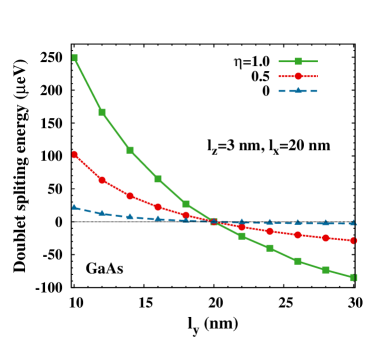
Figure 2: (Color online) The doublet splitting energies in single GaAs QD as function of the dot major/minor diameter $l_{y}$ with fixed minor/major diameter $l_{x}=20$ nm and dot height $l_{z}=3$ nm. Different values of $\eta$ are chosen to modulate the strength of the direct Coulomb interaction.

Table 2: Size parameters used in the calculation of doublet splitting energy in single InAs QD for Fig. 3(b).

	1	2	3	4	5	6	7
$l_{x}$ (nm)	21	19	17	15	14	13	12
$l_{z}$ (nm)	5.5	5.4	5.3	5.2	5.1	5	4.9
	8	9	10	11	12	13
$l_{x}$ (nm)	11.5	11	10.5	10	9.5	9
$l_{z}$ (nm)	4.8	4.75	4.7	4.55	4.5	4.4

Similar features of the shape dependence of doublet splitting energy are shown in Fig. 3(a) for InAs QDs with the direct Coulomb interaction fully included. In addition, we plot the doublet splitting energy as a function of the exciton recombination energy in Fig. 3(b) in order to compare with the experimental data by Seguin et al.Seguin . The exciton recombination energy is defined as $\frac{E_{X}+E_{Y}}{2}+E_{g}$, with $E_{g}$ standing for the band gap in cubic InAs. The experimental data are taken from Ref. Seguin, . In the calculation, we fix the major/minor diameter $l_{y}=10$ nm and vary the minor/major diameter $l_{x}$ in the range of $8.5\sim 20$ nm. The dot height $l_{z}$ is varied in the range of $4.3\sim 5.5$ nm. The exciton recombination energy is mainly modulated by the strong confinement along the $z$-direction while the doublet splitting energy is mainly determined by the ratio of $l_{x}:l_{y}$. So the theoretical points are obtained by properly choosing the values of ($l_{x}$, $l_{z}$) in pairs. From left to right in Fig. 3(b), the explicit values of ($l_{x}$, $l_{z}$) for the theoretical points are given in order in Table II. It is seen from the figure that our theoretical results are in good agreement with the experimental data. The doublet splitting energy decreases with increasing exciton recombination energy and intersects through zero. Generally speaking, we employ larger values of $l_{x}$ together with larger $l_{z}$, and hence smaller recombination energy. The zero point of doublet splitting energy is reached at $l_{x}=10$ nm and $l_{z}=4.55$ nm. In this way, the trend of the variation of the doublet splitting energy with the exciton recombination energy is well explained as a result of the dot geometry.note9

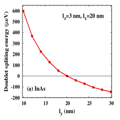
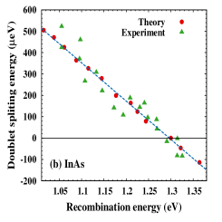
Figure 3: (Color online) The doublet splitting energy in single InAs QD (a) as a function of the dot major/minor diameter $l_{y}$ with fixed minor/major diameter $l_{x}=20$ nm and dot height $l_{z}=3$ nm; (b) as a function of the exciton recombination energy. The experimental points are taken from Ref. Seguin, and the theoretical points are calculated with the size parameters listed in Table II. The dotted line is plotted for the guide of eye.

The relative importance of the LR and SR exchange interactions with respect to the exciton fine structure splittings in QDs is an open question. Early work by Efros et al. included only the SR exchange interaction to investigate the band-edge excitons in spherical QDs. TakagaharaTaka2 assigned the origin of exciton doublet structure to the LR exchange interaction and Glazov et al.Ivchenko3 took into account only the LR exchange interaction in their work to investigate exciton fine structure in an anisotropic QD. However, Tsitsishvili et al.Kalt1 ; Kalt2 and Horodyská et al. in their very recent workHoro took into account only the SR exchange interaction for excitons in anisotropic and spherical QDs, respectively. Here we reexamine the relative importance of the LR and SR exchange interactions to the doublet splitting energy. Those to the BD exchange splitting are to be discussed in the following corresponding parts.

We calculate the doublet splitting energies by including the LR, SR and both LR and SR exchange interactions. In Fig. 4, we plot the doublet splittings as a function of the major/minor diameter $l_{y}$ with the minor/major diameter $l_{x}$ fixed in GaAs and InAs QDs. It is seen that the curves obtained by including the LR exchange interaction only and by including both the LR and SR exchange interactions almost match each other. The doublet splitting energies from the SR exchange interaction are always less than $1~{}\mu$eV, more than two orders of magnitude smaller than the splittings caused by the LR exchange interaction. So the LR exchange interaction is dominant in determining the doublet splitting energy when all heavy-hole, light-hole and split-off bands are taken into account. This is consistent with Ref. Taka2, where only the heavy- and light-hole bands are taken account of.

It is also noted that the doublet splitting energies from the SR exchange interaction are in opposite sign to those from the LR exchange interaction. This means that the relative positions of $|X\rangle$ and $|Y\rangle$ exciton states are reversed when only the SR exchange interaction is included.

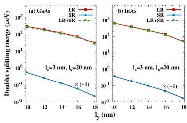
Figure 4: (Color online) The doublet splitting energies from the LR, SR and both LR and SR exchange interactions, are plotted as a function of the dot major/minor diameter $l_{y}$, with fixed minor/major diameter $l_{x}=20$ nm and dot height $l_{z}=3$ nm for (a) GaAs QD and (b) InAs QD.

We further investigate the size dependence of the doublet splittings of GaAs and InAs QDs and perform the 3D and 2D size-scaling analysis. Detailed results are plotted in Fig. 5 with the solid curves fit to the power law $\propto 1/L^{n}$. The results are consistent with the physical intuition. The doublet splitting energy increases with the decrease of the dot size since for smaller dot size, the overlap of the wave functions of electron and hole is enhanced and hence larger matrix elements of e-h exchange interaction are obtained [Eqs. (55) and (63) and their Hermitian conjugates]. We obtain $n_{\rm GaAs}=1.45$ and $n_{\rm InAs}=2.14$ in the 3D scaling and $n_{\rm GaAs}=1.04$ and $n_{\rm InAs}=1.6$ in the 2D scaling. All power indices obtained lie in the range of 1$\sim$3 and are consistent with the scaling rules for the LR exchange interaction established in Sec. II. The fact that the power indices of InAs QDs are larger than those of GaAs QDs is understood as follows. The exciton Bohr radius is 14.9 nm in bulk GaAs and 51.6 nm in bulk InAs. As compared to the characteristic size $L$ of the QDs in the 3D and 2D scalings, for GaAs QDs, $a_{\rm Bohr}^{\rm GaAs}$ is comparable to or smaller than $L$. So GaAs QDs are closer to the weak confinement limit. For InAs QDs, $a_{\rm Bohr}^{\rm InAs}$ is larger than $a_{\rm Bohr}^{\rm GaAs}$, so InAs QD is closer to the strong confinement limit compared to GaAs QD.

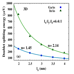
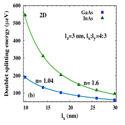
Figure 5: (Color online) The doublet splitting energies in GaAs and InAs QDs. (a) For the 3D scaling, with $l_{x}:l_{y}:l_{z}=6:4:1$. (b) For the 2D scaling, with $l_{x}:l_{y}=4:3$ and $l_{z}=3$ nm. The solid curves are fit to the power law $C/L^{n}$ and the index values $n$ are shown next to the curves.

III.1.2 BD exchange splitting

The band-edge exciton states in isotropic QDs were investigated in previous worksEfros ; Horo by including only the SR exchange interaction. It is noted that even though the doublet splitting energy, which is mainly from the LR exchange interaction, becomes zero in circular QDs, the LR exchange interaction still contributes to the splitting between the bright and dark exciton states. For circular GaAs QD with $l_{z}=3$ nm and $l_{x}=l_{y}=20$ nm, the BD exchange splitting is 1.76 meV and the LR exchange interaction contributes 0.17 meV to it. So in GaAs QDs, the SR exchange interaction is dominant in determining the BD exchange splitting. It is a different case in InAs QD of the same size, where the LR exchange interaction contributes 0.31 meV out of the total BD exchange splitting 0.49 meV. This difference is due to the fact that the singlet-triplet splitting parameter $\Delta E_{\rm SR}$ is 20 $\mu$eV in GaAs compared 0.3 $\mu$eV in InAs. As a result, the SR exchange interaction is rather weak in InAs. The calculated BD exchange splitting of 500 $\mu$eV in InAs QD with $l_{z}=6$ nm and $l_{x}=l_{y}=15$ nm is in good agreement with the experimental data.Bayer1 So we emphasize that the LR exchange interaction is important to understand the experimental results not only for the doublet splitting energy, but also for the BD exchange splitting in QDs.

Table 3: Power indices of the 2D and 3D scalings of the BD exchange splitting contributed by the LR, SR and both LR and SR exchange interactions in GaAs and InAs QDs.

		3D			2D
	LR	SR	Both	LR	SR	Both
GaAs	1.57	1.52	1.49	1.14	0.15	0.22
InAs	1.95	2.00	1.95	1.69	0.80	1.38

The size dependence of the BD exchange splitting is investigated in circular QDs for the purpose of eliminating the effect of doublet splitting. In the calculation, we take into account the LR, SR and both LR and SR exchange interactions. The results are shown in Fig. 6. The solid curves are fit to the power law $\propto 1/L^{n}$, and the obtained power indices of the size scaling of BD exchange splitting are listed in Table III. The size scaling laws of the BD exchange splitting by including only the LR exchange interaction are close to those of the doublet splitting energy in both the 3D and 2D scalings in GaAs and InAs QDs (see Fig. 6 and Table III). This is because the diagonal and off-diagonal matrix elements of the LR exchange interaction in Eq. (53) are in similar forms of the ${\bf r}$ dependence. The power indices of the BD exchange splitting from the SR exchange interaction lie reasonably in the range 1$\sim$3 in the 3D scaling and in the range 0$\sim$2 in the 2D scaling, and are consistent with the scaling rules established in Sec. II.

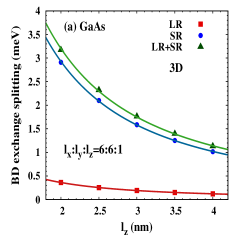
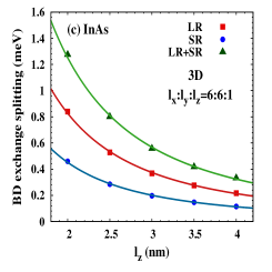
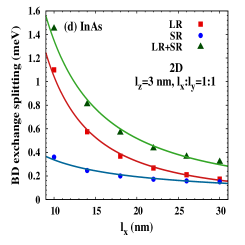
Figure 6: (Color online) The BD exchange splittings in circular QDs by taking account of the LR, SR and both LR and SR exchange interactions. (a) For the 3D scaling in GaAs QD, with $l_{x}:l_{y}:l_{z}=6:6:1$. (b) For the 2D scaling in GaAs QD with $l_{x}=l_{y}$ and $l_{z}=3$ nm. (c) For the 3D scaling in InAs QD, with $l_{x}:l_{y}:l_{z}=6:6:1$. (d) For the 2D scaling in InAs QD, with $l_{x}=l_{y}$ and $l_{z}=3$ nm. The solid curves are fit to the power law $C/L^{n}$ with $n$ listed in Table III.

An important feature of the relative energy positions of the dark and bright exciton states can be deduced from the above scalings. As in the 2D scalings, the power indices of the BD exchange splitting in isotropic GaAs and InAs QDs (also in GaN QD, see in the next subsection) are smaller than 2 in the size range under investigation. Meanwhile the level spacing between ground dark level and first excited dark level, which is induced by the lateral confinement, scales approximately as $\propto\frac{1}{L^{2}}$ [Eq. (123)].note5 So as the dot diameter increases, the first excited dark exciton level decreases more rapidly than the ground bright exciton level, and a crossing between these two levels may occur. For a typical case, in Fig. 7 we plot the eigenenergies of the ground dark exciton and bright exciton levels and the first excited dark exciton level as a function of the dot diameter $l_{x}$(=$l_{y}$) in GaAs QD. The dot height $l_{z}$ is fixed at 3 nm. When the dot diameter $l_{x}$ is varied from 10 to 30 nm, a crossing between the ground bright doublet and the first excited dark quartet (since $l_{x}=l_{y}$, the first excited dark exciton level is fourfold-degenerate) is observed around $l_{x}=23$ nm. This crossing can also be obtained in anisotropic QDs with the underlying physics.

This size-dependent bright-dark exciton level crossing provides a unique way of tuning the bright exciton states in resonance with the dark exciton states, which is meaningful to recent research on the optical nuclear spin pumping with the help of the hyperfine-interaction-mediated spin-flip transitions between the bright and dark exciton states.Klotz ; Chekhovich

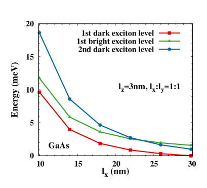
Figure 7: (Color online) The energy positions of the lowest dark and bright levels and the first excited dark level as function of $l_{x}$, with $l_{x}=l_{y}$ and $l_{z}=3$ nm. The zero point of energy is set at the lowest energy level at $l_{x}=30$ nm.

III.2 GaN

We then investigate the properties of the LR and SR exchange interactions in cubic GaN QD where theoretical works are absent. Compared to In_1-xGa_xAs-based structures, nanostructures based on GaN are less investigated both experimentally and theoretically. Much attention has been attracted for their unique properties, e.g., the wide band gap ($\sim$3.3 eV), which represents great potential for applications in electronics and photonics at temperature much higher than the liquid-helium or liquid-nitrogen cryogenic temperatures.Bardoux ; Kako ; Kindel

III.2.1 Doublet splitting

Due to the absence of experimental value of the singlet-triplet splitting $\Delta E_{\rm SR}$ in cubic GaN, the doublet splitting energy in GaN QDs is calculated by temporarily setting $\Delta E_{\rm SR}=20~{}\mu$eV.GaN-sr In Fig. 8(a), we plot the doublet splitting energies calculated by including the LR, SR and both LR and SR exchange interactions as a function of the dot minor diameter $l_{y}$. Similar to GaAs and InAs QDs, the SR exchange interaction is irrelevant when considering the doublet splitting energy. Since the strength of the SR exchange interaction is proportional to the value of $\Delta E_{\rm SR}$, we assert that $\Delta E_{\rm SR}$ in GaN can not be so large as to make the SR exchange interaction comparable or even exceed the LR exchange interaction because otherwise it will make other results, e.g., the BD exchange splitting, unreasonable. So in Fig. 8(b), we plot the doublet splitting energy varying with the dot shape, calculated without the SR exchange interaction. Size parameters are chosen according to the experiment.Marie One observes in the figure that with large anisotropy, the doublet splitting energy reaches 100s of $\mu$eV. The large doublet splitting energy obtained is key to understand the experiment by Lagarde et al.Marie where the conversion from exciton linearly polarized states $|X\rangle$ and $|Y\rangle$ to the circularly polarized ones $|\pm 1\rangle$ was not observed for magnetic field up to 4T.

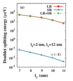
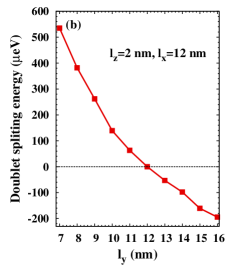
Figure 8: (Color online) The doublet splitting energies in single GaN QD as a function of the dot major/minor diameter $l_{y}$ with fixed minor/major diameter $l_{x}=12$ nm and dot height $l_{z}=2$ nm. (a) The doublet splitting energies from the LR, SR exchange interactions and both together; (b) the doublet splitting energy from the LR exchange interaction.

The size dependence of doublet splitting energy is also investigated. The obtained results can be well understood in a straightforward way as those for GaAs and InAs QDs discussed above. So we only plot our results in Fig. 9 without more discussions. The power indices obtained from the 2D and 3D size scalings are shown next to the curves. The scaling laws of doublet splitting energies found in GaN QDs are consistent with the rules established in Sec. II.

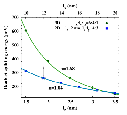
Figure 9: (Color online) The doublet splitting energies in GaN QDs. 1) For 3D scaling, with $l_{x}:l_{y}:l_{z}=6:4:1$. $l_{z}$ is varied from 1.5 to 3.5 nm. 2) For 2D scaling, with $l_{x}:l_{y}=4:3$ and $l_{z}=2$ nm. The solid curves are fit to the power law $C/L^{n}$ with the index values $n$ shown next to the curves. Note the scale of the 2D scaling is on top of the frame.

We further calculate the doublet splitting energy in small cubic GaN QDs by pushing our model to its extreme.note6 In Fig. 10, we plot the doublet splitting energies as function of dot size. It is seen that the doublet splitting energies reach several eV when the QDs become extremely small. This is strongly supported by recent experiment on wurtzite GaN QDs where doublet splitting energies in the range of 2$\sim$7 meV were reported.Kindel Further experiments on cubic GaN QDs are expected.

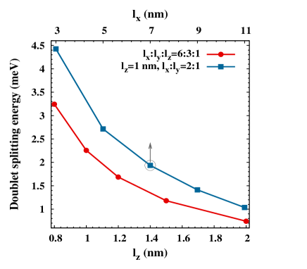
Figure 10: (Color online) The doublet splitting energies in small cubic GaN QDs as function of dot size. Note the scale of one of the curves is on top of the frame.

III.2.2 BD exchange splitting

Although the SR exchange interaction is negligible concerning the doublet splitting in GaN QDs, its contribution to the BD exchange splitting is still comparable to that of the LR exchange interaction. In order to investigate the properties of BD exchange splitting in GaN QDs, the singlet-triplet splitting $\Delta E_{\rm SR}$ is again set at $20~{}\mu$eV as a parameter.GaN-sr Due to the fact that in circular QDs, the BD exchange splitting calculated by including both the LR and SR exchange interactions is approximately the summation of those obtained by including each separately and the contribution of the SR exchange interaction is proportional to the value of $\Delta E_{\rm SR}$, the genuine value of $\Delta E_{\rm SR}$ in cubic GaN can be extracted by comparing our theoretical results of BD exchange splitting with future experimental data.

Table 4: Power indices of the 2D and 3D scaling of the BD exchange splitting contributed by the LR, SR and both LR and SR exchange interactions in GaN QDs.

		3D			2D
	LR	SR	Both	LR	SR	Both
GaN	1.76	1.74	1.75	1.26	0.22	0.68

In Fig. 11, we plot the BD exchange splitting as function of the dot size. The obtained power indices of size scaling are listed in Table IV. From Fig. 11(b), one observes a crossing of BD exchange splittings obtained from the LR exchange interaction and from the SR exchange interaction, indicating the exchange of the relative importance of the LR and the SR exchange interactions. This is due to the different scaling rules of the LR and SR exchange interactions in the 2D scaling [Eqs. (68), (72) and (70), (73)]. As the the dot diameter increases, the BD exchange splitting from the LR exchange interaction decreases more rapidly than that from the SR exchange interaction (see in Table IV for detailed values of power indices) and becomes smaller than it for $l_{x}>11.4$ nm in GaN QD. In fact, one may also expect a crossing in Fig. 6(d) in the region of $l_{x}>30$ nm in InAs QD.

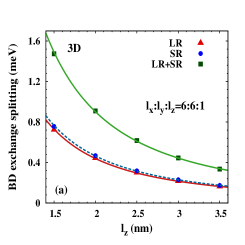
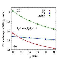
Figure 11: (Color online) The BD exchange splittings in GaN QDs by taking account of both the LR and SR exchange interactions, and separately: (a) for the 3D scaling, with $l_{x}:l_{y}:l_{y}=6:6:1$ and (b) for the 2D scaling, with $l_{x}=l_{y}$ and $l_{z}=2$ nm. The solid and dashed curves are fit to the power law $C/L^{n}$ and the index values $n$ are shown next to the curves.

III.3 Discussions on relative importance of the heavy-hole, light-hole and split-off bands

We now turn to address the relative importance of the heavy-hole, light-hole and split-off bands to the exciton fine structure. Theories of exciton fine structure in QDs were presented by taking into account only the heavy-hole band.Andreani ; Ivchenko4 It was pointed out by Takagahara that it is important to take account of the mixing of heavy-hole and light-hole bands to explain the experimental phenomena.Taka2 But this argument was not explicitly proved in that paper. In Fig. 12, we plot the energies of the lowest subbands of decoupled heavy, light and split-off holes in GaAs, InAs and GaN QWs. The valence band coupling is neglected so that $E_{z}=\frac{\hbar^{2}\pi^{2}}{2m_{z}^{\ast}l_{z}^{2}}$, with $m_{z}^{\ast}$ representing the effective mass of the heavy, light or split-off hole in the $z$-direction. The relative positions of these three subbands vary with $l_{z}$ because of different hole effective masses in the $z$-direction.Winkler As shown in the figure, in the strong confinement regime, the split-off subband is closer to the heavy-hole subband than the light-hole one for all three materials. Therefore, if the light-hole band is considered, the split-off band should also be included.

In order to investigate the relative importance of the heavy-hole, light-hole and split-off bands to the e-h exchange interaction, the doublet splitting energy and the BD exchange splitting are calculated by taking into account: (i) the heavy-hole band only; (ii) heavy-hole and light-hole bands; and (iii) all the three valence bands, separately. In Fig. 13, we plot the doublet splittings originated from the three valence bands separately. The contribution of the heavy-hole band is calculated by including the terms of e-h exchange interaction derived from the heavy-hole band only as in Case (i). The contribution from the light-hole (split-off) band is obtained by subtracting the splitting calculated from Case (i) [Case (ii)] from the one from Case (ii) [Case (iii)]. It is noted that the doublet splitting energy is decreased by further including the light-hole and split-off bands. Therefore in Fig. 13, the contributions from the light-hole and split-off bands are multiplied by $-1$. Moreover, for GaN QDs, the structure splittings are calculated by setting $\Delta E_{\rm SR}=20~{}\mu$eV.GaN-sr As shown in the figure, the contribution of the heavy-hole band is much larger than those from the other two bands. The doublet splitting energy is slightly changed by further including the light-hole and split-off bands as in Case (ii) and (iii), with the split-off band contributing most of the change. Under all size parameters adopted, the doublet splitting energy is only changed by less than 2 $\%$ in both GaAs and GaN QDs, and less than $7.2~{}\%$ in InAs QDs. One can hence conclude that the terms derived from the heavy-hole band dominate the off-diagonal matrix elements of the LR exchange interaction [Eq. (55) and its Hermitian conjugate], i.e., $|S_{ij}|\ll 1$. And they are also much larger than the off-diagonal matrix elements of the SR exchange interaction [i.e., Eq. (63) and its Hermitian conjugate].

Similarly, we find that the contribution of light-hole and split-off bands to the BD exchange splitting is also small, in the order of $1~{}\mu$eV, which is much smaller than 100s of $\mu$eV from the heavy-hole band for all three materials under investigation. This can be understood in the same way: according to Eqs. (53)-(64), for the LR exchange interaction, terms without $S_{ij}$ and $S^{\prime\ast}_{ij}$ should also dominate the diagonal matrix elements of the LR exchange interaction which contribute to the BD exchange splitting. Moreover, for the SR exchange interaction, the diagonal matrix elements [Eqs. (62) and (64)] are not affected by the inclusion of the light-hole and split-off bands up to the order under consideration.

In short, both the light-hole and split-off bands are negligible when the band-edge exciton fine structure is investigated in cubic III-V semiconductor QDs with strong confinement along the [001] direction. This further demonstrates the feasibility of treating the light-hole and split-off bands perturbatively through the Löwdin partition. However, as discussed after Eqs. (47) and (48), the confinement-induced valence band mixing is crucial in understanding some exciton properties, e.g., the observability of the dark excitonBayer1 ; Bayer3 ; Gorycal ; Nirmal and the degree of the linear polarization of QD emission.Leger

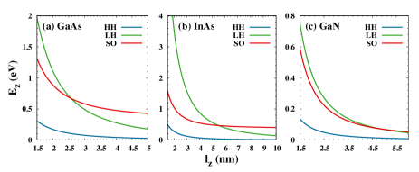
Figure 12: (Color online) Eigenenergies of decoupled heavy-hole (HH), light-hole (LH) and split-off-hole (SO) ground states in QW. Infinite square well potential is employed and the well width is denoted as $l_{z}$. (a) GaAs, (b) InAs, (c) GaN.

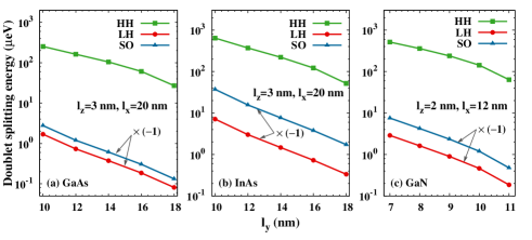
Figure 13: (Color online) Contributions of the heavy-hole (HH), light-hole (LH) and split-off (SO) bands to the doublet splitting energy, calculated as a function of the dot minor diameter $l_{y}$, with fixed dot major diameter $l_{x}=20$ nm and dot height $l_{z}=3$ nm for (a) GaAs QD, (b) InAs QD; and with $l_{x}=12$ nm and $l_{z}=2$ nm for (c) GaN QD.

IV Exciton spin relaxation in GaN QDs

In this section, we study the exciton spin relaxation in single GaN QDs. The relaxation rate is calculated from the Fermi golden rule with the exciton eigenfunctions and eigenenergies obtained from the exact diagonalization method.note7 Since the ground state of the bright exciton is polarized along the major axis of the potential ellipse, the relaxation rate is calculated from the upper state of the doublet to the lower one, i.e., $|Y\rangle\rightarrow|X\rangle$ for $l_{x}>l_{y}$ and $|X\rangle\rightarrow|Y\rangle$ for $l_{x}<l_{y}$.

In the calculation, we fix the major/minor diameter $l_{x}=12$ nm and the dot height $l_{z}=2$ nm.Marie The shape dependence of the exciton spin relaxation rate is studied by varying the minor/major diameter $l_{y}$ and the results are plotted in Fig. 14. One observes from the figure that the relaxation rate between the lowest $|X\rangle$ and $|Y\rangle$ exciton states shows strong dependence on the dot anisotropy. In the regime of large anisotropy, the relaxation rate reaches $10^{4}~{}\mu$s^-1, which in turn gives the exciton spin relaxation time in the order of 10 ps. In the vicinity of $l_{y}=l_{x}$, the relaxation rate decreases quickly with decreasing dot anisotropy. When the QD approaches the circular shape, the rate of change is even larger. The relaxation rate decreases down to less than $100$ s^-1 and tends to zero when $l_{y}$ approaches $l_{x}$. This calculated long exciton spin relaxation time, especially in the range of $l_{y}$ 11$\sim$13 nm, is supported by the latest experiment.Marie

It is pointed out that the behavior of spin relaxation rate in the range of $l_{y}=7\sim$16 nm mostly results from the anisotropy dependence of doublet splitting energy shown in Fig. 8(b). From Eq. (74), one has

$$\Gamma_{i\to f}=\frac{2\pi}{\hbar}\sum_{\lambda}\int d\theta d\phi q_{\lambda}^{2}|M_{{\bf q}_{\lambda}}|^{2}|\langle f|\chi({\bf q}_{\lambda})|i\rangle|^{2}.$$ (79)

When the wave vector $q_{\lambda}$ is not too large, the value of the relaxation rate is mainly modulated by the factor $q_{\lambda}^{2}|M_{{\bf q}\lambda}|^{2}$, which increases with increasing $q_{\lambda}$ for all three channels under consideration. The wave vector of the acoustic phonon is given by $q_{\lambda}=\frac{\Delta E}{\hbar v_{\lambda}}$, with $v_{\lambda}$ representing the sound velocity and $\Delta E$ denoting the phonon energy, which is equal to the difference of eigenenergies between the two bright exciton states considered, i.e., the doublet splitting energy. One observes from Fig. 8(b) that qualitatively, the doublet splitting energy is proportional to the dot anisotropy. So large dot anisotropy indicates large phonon wave vector, which in turn results in the anisotropy dependence of relaxation rate as shown in Fig. 14 in the range of $l_{y}=7\sim 16$ nm.

With further decrease of $l_{y}$ down to less than 7 nm, the exciton spin relaxation rate reaches a maximum around $l_{y}=6$ nm, where the doublet splitting energy is about $730~{}\mu$eV which corresponds to the situation that the wavelength of the emissive phonon becomes comparable with twice of the lateral dot size.Ka ; Bockelmann On the other side, when $l_{y}$ increases over 16 nm, the increase of the relaxation rate becomes slower and when $l_{y}$ reaches 24 nm, the relaxation rate also reaches a maximum. The underlying physics is different from the previous one. Here, the maximum is attributed to the interplay of the dot anisotropy and the strength of the lateral confinement. On one hand, the increase of $l_{y}$ gives a more anisotropic dot shape which tends to increase the doublet splitting energy; on the other hand, the confinement along the $y$-direction becomes weaker with larger $l_{y}$, which tends to decrease the overlap of the electron and hole wave functions and reduce the doublet splitting energy according to Eq. (55). The competing leads to the maximum.

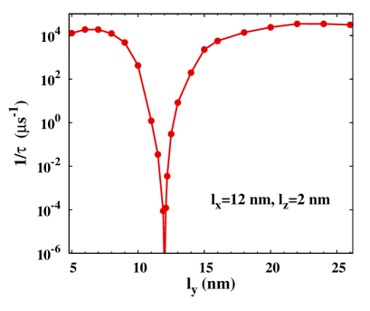
Figure 14: The dependence of relaxation rate between the lowest $|X\rangle$ and $|Y\rangle$ bright exciton states on the dot major/minor diameter $l_{y}$ with fixed minor/major diameter $l_{x}=12$ nm and dot height $l_{z}=2$ nm.

In addition, the relative importance of the three channels contributing to the exciton relaxation rate is investigated. We take into account one channel at a time and the results are plotted in Fig. 15. It is seen that the relaxation rate limited by the electron/hole-longitudinal acoustic phonon scattering due to the piezoelectric field coupling is always 1 to 3 orders of magnitude larger than that due to the deformation potential, but is 2 to 3 orders of magnitude smaller than the one limited by the electron/hole-transverse acoustic phonon scattering due to the piezoelectric coupling. So the transverse acoustic phonon-emission process dominates the exciton spin relaxation between the lowest $|X\rangle$ and $|Y\rangle$ bright exciton states in GaN QDs.

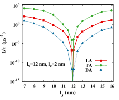
Figure 15: (Color online) The relaxation rate limited by the electron/hole-longitudinal acoustic phonon scatterings due to the deformation potential (DA) and the piezoelectric coupling  (LA), and by the electron/hole-transverse acoustic phonon scattering due to the piezoelectric coupling (TA). The relaxation rates are plotted as function of the dot major/minor diameter $l_{y}$ with fixed minor/major diameter $l_{x}=12$ nm and dot height $l_{z}=2$ nm.

V SUMMARY

In summary, we have established a general scheme to investigate the exciton fine structure and spin relaxation in cubic III-V semiconductor QDs. A $12\times 12$ matrix representation of the exciton Hamiltonian corresponding to the LR and SR exchange interactions is derived by taking into account the conduction band $\Gamma_{6}^{c}$, the heavy-hole and light-hole bands $\Gamma_{8}^{v}$ and the split-off band $\Gamma_{7}^{v}$, where the split-off band has never been included explicitly to investigate the exciton properties. In the case with strong confinement in one direction (the [001] direction in this paper), the Löwdin partitioning method is employed to take account of the confinement-induced band mixing and a four-band Hamiltonian of the e-h exchange interaction is derived. We use these formulae in the study of the relative importance of the heavy-hole, light-hole and split-off bands to the exciton fine structure. We find that the contribution of the split-off band is a little larger than that of the light-hole band, but both are negligible when considering the exciton fine structure in GaAs, InAs and GaN QDs. This behavior in GaN QDs is unexpected since a significant effect of the split-off band is expected due to the large band gap and the small spin-orbit splitting in cubic GaN. We attribute this to the confinement-induced subband splitting due to the different effective masses of the heavy, light and split-off holes in the $z$ direction.

In our approach, the direct Coulomb interaction is treated unperturbatively. We find that the strength of the direct Coulomb interaction strongly affects the doublet splitting energy (hence also the BD exchange splitting). We also show that previous works in which the direct Coulomb interaction was treated perturbatively vastly underestimate the doublet splitting. We demonstrate that the exact inclusion of the direct Coulomb interaction is important for excitons in the weak confinement regime.note2

We also discuss the size and shape dependences of the doublet splitting energy and the BD exchange splitting. Strong anisotropy dependence of the doublet splitting energy is reported, which agrees with the former theoretical and experimental works on GaAs and InAs QDs.Seguin ; Taka2 The size dependences of the doublet splitting energy and the BD exchange splitting are investigated by performing the size-scaling analysis. The behavior of the variation of the fine structure splittings with the dot size is well explained by the scaling rules established. The doublet splitting energy in cubic GaN QDs increases with the increase of dot anisotropy and/or the decrease of dot size, varying from 0 to 100s of $\mu$eV, and reaching up to several meV for extremely small dot size and large dot anisotropy. Our results are well supported by recent experimental findingsMarie ; Kindel but call for more experimental works. The still undetermined singlet-triplet splitting $\Delta E_{\rm SR}$ in cubic GaN can be fit from future experimental data on the BD exchange splitting, but the uncertainty does not affect the conclusions of this paper.

We investigate the relative importance of the LR and SR exchange interactions to the exciton fine structure. The LR exchange interaction is identified as the origin of the exciton doublet structure, which is in agreement with that by TakagaharaTaka2 where only the heavy- and light-hole bands were included. We show that the LR exchange interaction, which is absent in many previous works,Efros ; Horo contributes to the splitting between the bright and dark exciton states, even in circular QDs where the doublet splitting vanishes. The contribution of the LR exchange interaction to the BD exchange splitting is smaller than that of the SR one in GaAs QDs but is comparable in InAs and GaN QDs. Our calculations also demonstrate that the relative importance of the LR and SR exchange interactions to the BD exchange splitting can exchange with the variation of the dot lateral size.

The exciton spin relaxation in cubic GaN QDs is also investigated. We find that the exciton spin relaxation rate strongly depends on the dot anisotropy (relaxation rate from $10^{4}~{}\mu$s^-1 down to less than $10^{-4}~{}\mu$s^-1 is reported). In the small anisotropy regime, the long exciton spin relaxation time obtained (longer than 100 ns) is in good agreement with recent experiment by Lagarde et al..Marie The electron/hole-transverse acoustic phonon scattering due the piezoelectric field is recognized as the dominant magnetism of the exciton spin relaxation.

Finally, we address the possible extensions of our work: (a) Other than the shape anisotropy of QDs, strain anisotropy can also result in the doublet splitting, which is not included in the present investigation. (b) Within our model, the infinite square well potential is employed as the confinement along the $z$ direction and only the lowest electron and hole subband is included. As pointed out in Ref. note6, , in the case of extremely small QDs, one needs to switch to other model potential or approach such as the psudopotential approximationZunger2 ; Bester1 ; Bester2 to obtain more accurate results. Meanwhile, for QDs, the vertical height of which is not much smaller than its lateral size or the exciton Bohr radius, the multi-subband effect has to be included. (c) The fine structure splittings may also be modulated by external electric and/or magnetic fields which are not discussed in this paper. (d) Our model can also be extended to investigate the initial optical spin polarizations.Marie2 ; Pfalz ; Kowa

Appendix A The Exciton Hamiltonian

Here we write down the explicit form of the exciton Hamiltonian $H^{\rm eh}_{m^{\prime}n^{\prime}\atop mn}\left({\bf r}^{\prime}_{1}\ {\bf r}^{\prime}_{2}\atop{\bf r}_{1}\ {\bf r}_{2}\right)$ in Eq. (2), which is recovered following the way laid out by Pikus and BirBir1 ; Bir2

$$H^{\rm eh}_{m^{\prime}n^{\prime}\atop mn}\left({\bf r}^{\prime}_{1}\ {\bf r}^{\prime}_{2}\atop{\bf r}_{1}\ {\bf r}_{2}\right)=\left[H^{e}_{m^{\prime}m}({\bf k}_{1})\delta_{n^{\prime}n}+H^{h}_{n^{\prime}n}({\bf k}_{2})\delta_{m^{\prime}m}\right.$$

$$\ \ \ \ \ \ \left.\mbox{}+U^{\rm eh}({\bf r}_{1}-{\bf r}_{2})\delta_{m^{\prime}m}\delta_{n^{\prime}n}\right]\delta({\bf r}_{1}-{\bf r}^{\prime}_{1})\delta({\bf r}_{2}-{\bf r}^{\prime}_{2})$$

$$\ \ \ \ \ \ \mbox{}+\Delta U^{{\rm ex}}_{m^{\prime}n^{\prime}\atop mn}\left({\bf r}^{\prime}_{1}\ {\bf r}^{\prime}_{2}\atop{\bf r}_{1}\ {\bf r}_{2}\right),$$ (80)

where ${\bf k}=-i\bigtriangledown$ and

$$U^{\rm eh}({\bf r}_{1}-{\bf r}_{2})=-\frac{e^{2}}{4\pi\varepsilon_{0}\kappa|{\bf r}_{1}-{\bf r}_{2}|},$$ (81)

$$H^{e}_{m^{\prime}m}({\bf k}_{1})=\Big{[}E_{m}({\bf k}_{0})+\frac{\hbar^{2}}{2m}{\bf k}_{1}^{2}\Big{]}+\frac{\hbar}{m}({\bf k}_{1}\cdot{\bm{\pi}}_{m^{\prime}m})$$

$$\mbox{}+\frac{\hbar^{2}}{m^{2}}\sum_{n^{\prime\prime}}\frac{({\bf k}_{1}\cdot{\bm{\pi}}_{m^{\prime}n^{\prime\prime}})({\bf k}_{1}\cdot{\bm{\pi}}_{n^{\prime\prime}m})}{E^{0}_{m}-E^{0}_{n^{\prime\prime}}},$$ (82)

$$H^{h}_{n^{\prime}n}({\bf k}_{2})=-H^{e}_{\Theta n\Theta n^{\prime}}(-{\bf k}_{2})=-H^{e}_{n^{\prime}n}({\bf k}_{2}).$$ (83)

Here $H^{e}_{m^{\prime}m}$ is in the usual form derived from the ${\bf k}\cdot{\bf p}$ method up to the second order. We have ${\bm{\pi}}={\bf p}+\frac{\hbar}{4mc^{2}}\left[{\bm{\sigma}}\times(\bigtriangledown V_{0})\right]$ with $V_{0}$ standing for the lattice potential. ${\bm{\pi}}_{mn}$ denotes the matrix element of ${\bm{\pi}}$ between the two Bloch functions $\psi_{m{\bf k}_{0}}({\bf r})$ and $\psi_{n{\bf k}_{0}}({\bf r})$. In this paper, lattice potential $V_{0}$ is assumed to have spherical symmetry. $\Theta$ stands for the time reversal operator.

The e-h exchange interaction is decomposed into LR and SR parts:

$$\Delta U^{{\rm ex}}_{m^{\prime}n^{\prime}\atop mn}\left({\bf r}^{\prime}_{1}\ {\bf r}^{\prime}_{2}\atop{\bf r}_{1}\ {\bf r}_{2}\right)=H^{{\rm LR}}_{m^{\prime}n^{\prime}\atop mn}\left({\bf r}^{\prime}_{1}\ {\bf r}^{\prime}_{2}\atop{\bf r}_{1}\ {\bf r}_{2}\right)+H^{{\rm SR}}_{m^{\prime}n^{\prime}\atop mn}\left({\bf r}^{\prime}_{1}\ {\bf r}^{\prime}_{2}\atop{\bf r}_{1}\ {\bf r}_{2}\right),$$ (84)

with

$$H^{{\rm LR}}_{m^{\prime}n^{\prime}\atop mn}\left({\bf r}^{\prime}_{1}\ {\bf r}^{\prime}_{2}\atop{\bf r}_{1}\ {\bf r}_{2}\right)=-\sum_{\alpha\beta}Q^{\alpha\beta}_{m^{\prime}\Theta n\atop\Theta n^{\prime}m}\frac{\partial^{2}}{\partial{\bf r}^{\alpha}_{1}\partial{\bf r}^{\beta}_{1}}U({\bf r}_{1}-{\bf r}^{\prime}_{2})$$

$$\ \ \ \ \ \ \mbox{}\times\delta({\bf r}_{1}-{\bf r}_{2})\delta({\bf r}^{\prime}_{1}-{\bf r}^{\prime}_{2}),$$ (85)

$$H^{{\rm SR}}_{m^{\prime}n^{\prime}\atop mn}\left({\bf r}^{\prime}_{1}\ {\bf r}^{\prime}_{2}\atop{\bf r}_{1}\ {\bf r}_{2}\right)={\cal V}U_{m^{\prime}\Theta n\atop\Theta n^{\prime}m}\delta({\bf r}_{1}-{\bf r}_{2})\delta({\bf r}_{1}-{\bf r}^{\prime}_{1})$$

$$\ \ \ \ \ \ \mbox{}\times\delta({\bf r}_{2}-{\bf r}^{\prime}_{2}).$$ (86)

In these equations, we have

$$Q^{\alpha\beta}_{m^{\prime}\Theta n\atop\Theta n^{\prime}m} = \frac{\hbar^{2}}{m^{2}}\frac{\pi^{\alpha}_{m^{\prime}\Theta n^{\prime}}\pi^{\beta}_{\Theta nm}}{(E_{m}^{0}-E_{n}^{0})(E_{m^{\prime}}^{0}-E_{n^{\prime}}^{0})},$$ (87)

$$U({\bf r}) = \frac{e^{2}}{4\pi\varepsilon_{0}\kappa|{\bf r}|},$$ (88)

and $E_{s}^{0}$ represents the eigenenergy of the $s$ band at the point ${\bf k}={\bf k}_{0}$; ${\cal V}$ is the volume of the bulk material which comes from the normalization of the Bloch function and

$$U_{m^{\prime}\Theta n\atop\Theta n^{\prime}m}=\frac{1}{{\cal V}^{2}}\int\int\psi^{\ast}_{m^{\prime}{\bf k}_{0}}({\bf r}_{1})(\Theta\psi_{n{\bf k}_{0}}({\bf r}_{2}))^{\ast}U({\bf r}_{1}-{\bf r}_{2})$$

$$\ \ \ \ \ \ \mbox{}\times\Theta\psi_{n^{\prime}{\bf k}_{0}}({\bf r}_{1})\psi_{m{\bf k}_{0}}({\bf r}_{2})d{\bf r}_{1}d{\bf r}_{2}.$$ (89)

Appendix B The Bloch Functions

The Bloch functions of the $\Gamma_{6}^{c}$ conduction band take the formWinkler

$$|\frac{1}{2},\frac{1}{2}\rangle_{c}=|S\rangle\alpha,\ |\frac{1}{2},-\frac{1}{2}\rangle_{c}=|S\rangle\beta.$$ (90)

where $\alpha$ ($\beta$) denotes the spin-up (down) state and $|S\rangle$ represents the $s$-like conduction band Bloch function. The Bloch functions of the $\Gamma_{8}^{v}$ and $\Gamma_{7}^{v}$ valence bands are written asWinkler

$$|\frac{3}{2},\frac{3}{2}\rangle_{v}=-\frac{1}{\sqrt{2}}(|X\rangle+i|Y\rangle)\alpha,$$ (91)

$$|\frac{3}{2},\frac{1}{2}\rangle_{v}=\frac{1}{\sqrt{6}}\big{[}-(|X\rangle+i|Y\rangle)\beta+2|Z\rangle\alpha\big{]},$$ (92)

$$|\frac{3}{2},-\frac{1}{2}\rangle_{v}=\frac{1}{\sqrt{6}}\big{[}(|X\rangle-i|Y\rangle)\alpha+2|Z\rangle\beta\big{]},$$ (93)

$$|\frac{3}{2},-\frac{3}{2}\rangle_{v}=\frac{1}{\sqrt{2}}(|X\rangle-i|Y\rangle)\beta,$$ (94)

$$|\frac{1}{2},\frac{1}{2}\rangle_{v}=-\frac{1}{\sqrt{3}}\big{[}({|X\rangle+i|Y\rangle})\beta+|Z\rangle\alpha\big{]},$$ (95)

$$|\frac{1}{2},-\frac{1}{2}\rangle_{v}=-\frac{1}{\sqrt{3}}\big{[}({|X\rangle-i|Y\rangle})\alpha-|Z\rangle\beta\big{]},$$ (96)

where $|X\rangle$, $|Y\rangle$ and $|Z\rangle$ are the $p$-like valence band Bloch functions which are real according to the phase convention in accordance with the time-reversal symmetry. After taking the time reversal operation, we have

$$\Theta|\frac{3}{2},\frac{3}{2}\rangle_{v}=-\frac{1}{\sqrt{2}}(|X\rangle-i|Y\rangle)\beta,$$ (97)

$$\Theta|\frac{3}{2},\frac{1}{2}\rangle_{v}=\frac{1}{\sqrt{6}}\big{[}(|X\rangle-i|Y\rangle)\alpha+2|Z\rangle\beta\big{]},$$ (98)

$$\Theta|\frac{3}{2},-\frac{1}{2}\rangle_{v}=\frac{1}{\sqrt{6}}\big{[}(|X\rangle+i|Y\rangle)\beta-{2}|Z\rangle\alpha\big{]},$$ (99)

$$\Theta|\frac{3}{2},-\frac{3}{2}\rangle_{v}=-\frac{1}{\sqrt{2}}(|X\rangle+i|Y\rangle)\alpha,$$ (100)

$$\Theta|\frac{1}{2},\frac{1}{2}\rangle_{v}=\frac{1}{\sqrt{3}}\big{[}({|X\rangle-i|Y\rangle})\alpha-|Z\rangle\beta\big{]},$$ (101)

$$\Theta|\frac{1}{2},-\frac{1}{2}\rangle_{v}=-\frac{1}{\sqrt{3}}\big{[}({|X\rangle+i|Y\rangle})\beta+|Z\rangle\alpha\big{]}.$$ (102)

Appendix C Construction of basis functions with direct Coulomb interaction explicitly included

With the confinement, the diagonal part of the exciton Hamiltonian $H^{\rm eh}_{m^{\prime}n^{\prime}\atop mn}\left({\bf r}^{\prime}_{1}\ {\bf r}^{\prime}_{2}\atop{\bf r}_{1}\ {\bf r}_{2}\right)$, i.e., excluding the e-h exchange interaction, can be written into

$$H_{D}=H_{e}+H_{h}+H_{\rm Coulomb}+H_{\rm confinement},$$ (103)

where $H_{e}$ is the electron Hamiltonian in the form $H_{e}=\hbar^{2}k_{e}^{2}/2m_{e}^{\ast}$ with $m_{e}^{\ast}$ being the effective mass of the conduction electron and $H_{h}$ is the hole Hamiltonian. From Eq. (40), we see that $H_{h}$ is diagonal in the 4$\times$4 matrix representation and the quasi-spins are not coupled. So in the following we omit the spin degree of freedom of both electron and hole. $H_{\rm Coulomb}$ and $H_{\rm confinement}$ are the direct Coulomb interaction and the confinement potential, given in Eq. (81) and Eqs. (77)-(78). The eigen equation for the envelope basis function is constructed as

$$H_{D}|{\rm eh}\rangle = E|{\rm eh}\rangle,$$ (104)

$$\langle{\bf r}_{1},{\bf r}_{2}|{\rm eh}\rangle = f({\bf r}_{1},{\bf r}_{2}).$$ (105)

When a strong confinement is applied along the $z$-direction so that only the lowest electron/hole subband is relevant, one has

$$f({\bf r}_{1},{\bf r}_{2})=\Phi({\bf r}_{1||},{\bf r}_{2||})\xi(z_{1})\zeta(z_{2}),$$ (106)

where $\xi(z)[\zeta(z)]=\sqrt{\frac{2}{l_{z}}}{\rm sin}(\frac{\pi z}{l_{z}})$ stands for the electron (hole) envelope function in the $z$-direction. After multiplying both sides of Eq. (104) with $\xi(z_{1})\zeta(z_{2})$ and integrating over $z_{1}$ and $z_{2}$, one comes to

$$\tilde{H}_{D}\Phi({\bf r}_{1\parallel},{\bf r}_{2\parallel})=E\Phi({\bf r}_{1\parallel},{\bf r}_{2\parallel}),$$ (107)

with

$$\tilde{H}_{D}=\frac{p_{1\parallel}^{2}}{2m_{e}^{\ast}}+\frac{p_{2\parallel}^{2}}{2m_{h\parallel}^{\ast}}+\frac{1}{2}m_{e}^{\ast}(\omega_{xe}^{2}x_{1}^{2}+\omega_{ye}^{2}y_{1}^{2})$$

$$\ \ \ \mbox{}+\frac{1}{2}m_{h\parallel}^{\ast}(\omega_{xh}^{2}x_{2}^{2}+\omega_{yh}^{2}y_{2}^{2})+V({\bf r}_{\parallel})+E_{z}^{e}+E_{z}^{h},$$ (108)

in which

$$m_{h\parallel}^{\ast}=\frac{m_{0}}{\gamma_{1}+\gamma_{2}},\ \ E_{z}^{e}=\frac{\hbar^{2}\pi^{2}}{2m_{e}^{\ast}l_{z}^{2}},\ E_{z}^{h}=\frac{\hbar^{2}\pi^{2}}{2m_{h,z}^{\ast}l_{z}^{2}},$$ (109)

$$m_{h,z}^{\ast}=\frac{m_{0}}{\gamma_{1}-2\gamma_{2}},\ \ {\bf r}_{\parallel}=(x_{1}-x_{2},y_{1}-y_{2}),$$ (110)

$$V({\bf r}_{\parallel})=\frac{4}{l_{z}^{2}}\int_{0}^{l_{z}}dz_{1}\int_{0}^{l_{z}}dz_{2}U^{\rm eh}({\bf r}_{1}-{\bf r}_{2})$$

$$\hskip 5.69046pt\mbox{}\times[{\rm sin}({\pi z_{1}}/{l_{z}}){\rm sin}({\pi z_{2}}/{l_{z}})]^{2}.$$ (111)

Here, $m_{h\parallel}^{\ast}$ and $m_{h,z}^{\ast}$ are the effective masses of the heavy-hole in the plane and in the $z$-direction, respectively; $E_{z}^{e}$ and $E_{z}^{h}$ are the subband energies resulting from the strong confinement in the $z$-direction.

After separating the coordinates of electron-hole pair in the plane into the center-of-mass and relative parts:

$$\begin{array}[]{ll}{\bf r}_{\parallel}={\bf r}_{1\parallel}-{\bf r}_{2\parallel}\\ {\bf R}_{\parallel}=\frac{m_{e}^{\ast}{\bf r}_{1\parallel}+m_{h\parallel}^{\ast}{\bf r}_{2\parallel}}{m_{e}^{\ast}+m_{h\parallel}^{\ast}}\end{array}\Longrightarrow\left\{\begin{array}[]{ll}{\bf K}_{\parallel}={\bf k}_{1\parallel}+{\bf k}_{2\parallel}\\ {\bf k}_{\parallel}=\frac{m_{h\parallel}^{\ast}{\bf k}_{1\parallel}-m_{e}^{\ast}{\bf k}_{2\parallel}}{m_{e}^{\ast}+m_{h\parallel}^{\ast}}\end{array},\right.$$ (112)

$\tilde{H}_{D}$ is separated into two parts: $\tilde{H}_{D}=\tilde{H}_{0}+\tilde{H}^{\prime}$, where

$$\tilde{H}_{0}=\frac{\hbar^{2}}{2m_{\mu}}(k_{x}^{2}+k_{y}^{2})+\frac{1}{2}m_{\mu}\omega_{\rm ave}^{2}(x^{2}+y^{2})$$

$$\mbox{}+\frac{1}{2}{m_{0}^{2}}\big{(}\frac{1}{m_{e}^{\ast}}+\frac{1}{m_{h\parallel}^{\ast}}\big{)}(\omega_{x0}^{2}X^{2}+\omega_{y0}^{2}Y^{2})$$

$$\mbox{}+\frac{\hbar^{2}}{2(m_{e}^{\ast}+m_{h\parallel}^{\ast})}(K_{x}^{2}+K_{y}^{2})+V(r_{\parallel}),$$ (113)

in which

$$m_{\mu}=\frac{m_{e}^{\ast}m_{h\parallel}^{\ast}}{m_{e}^{\ast}+m_{h\parallel}^{\ast}},\ \ \omega_{\rm ave}^{2}=\frac{\omega_{xr}^{2}+\omega_{yr}^{2}}{2},$$ (114)

$$\omega_{xr}=\hbar\Big{(}{\frac{m_{e}^{\ast}m_{h\parallel}^{\ast}}{\sqrt{m_{e}^{\ast 2}-m_{e}^{\ast}m_{h\parallel}^{\ast}+m_{h}^{\ast 2}}}l_{x}^{2}}\Big{)}^{-1},$$ (115)

$$\omega_{yr}=\hbar\Big{(}{\frac{m_{e}^{\ast}m_{h\parallel}^{\ast}}{\sqrt{m_{e}^{\ast 2}-m_{e}^{\ast}m_{h\parallel}^{\ast}+m_{h}^{\ast 2}}}l_{y}^{2}}\Big{)}^{-1}.$$ (116)

$\tilde{H}^{\prime}$ is further constituted of two parts:

$$\tilde{H}^{\prime}=H_{L1}+H_{L2},$$ (117)

with

$$H_{L1}=m_{0}^{2}(\frac{b}{m_{e}^{\ast}}-\frac{a}{m_{h\parallel}^{\ast}})(\omega_{x0}^{2}xX+\omega_{y0}^{2}yY),$$ (118)

$$H_{L2}=\frac{1}{2}m_{\mu}\left[(\omega_{xr}^{2}-\omega_{\rm ave}^{2})x^{2}+(\omega_{yr}^{2}-\omega_{\rm ave}^{2})y^{2}\right],$$ (119)

where

$$a=\frac{m_{e}^{\ast}}{m_{e}^{\ast}+m_{h\parallel}^{\ast}},\ \ \ b=\frac{m_{h\parallel}^{\ast}}{m_{e}^{\ast}+m_{h\parallel}^{\ast}},$$ (120)

$$\omega_{x0}=\frac{\hbar}{m_{0}l_{x}^{2}},\ \ \ \ \ \ \omega_{y0}=\frac{\hbar}{m_{0}l_{y}^{2}}.$$ (121)

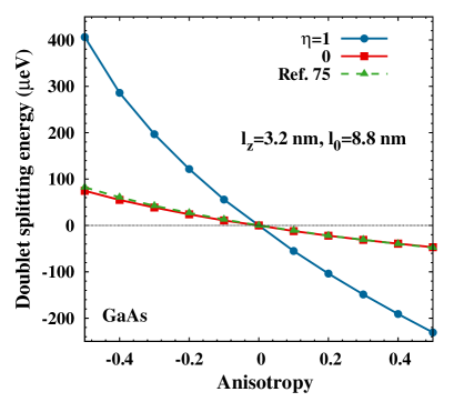
Figure 16: (Color online) The dependence of doublet splitting energy on the dot anisotropy in an GaAs QD with $l_{z}=3.2$ nm and $l_{0}=8.8$ nm. $\eta$ is set at 1 or 0 to switch the direct Coulomb interaction on and off. The triangle points are taken from Fig. 2 in Ref. Kada, .

Treating $\tilde{H}^{\prime}$ perturbatively, we see from Eq. (113) that the center-of-mass and relative motions of the electron-hole pair are now decoupled and we are able to write the in-plane wave function as $\Phi({\bf r}_{1\parallel},{\bf r}_{h\parallel})=\psi(X,Y)\varphi({\bf r}_{\parallel})$. Here $\psi$ is the eigenfunction of the 2D harmonic-oscillator potential

$$\psi_{n_{x}n_{y}}(X,Y)=A_{n_{x}}A_{n_{y}}e^{-(\alpha_{c}^{2}X^{2}+\beta_{c}^{2}Y^{2})/2}H_{n_{x}}(\alpha_{c}X)$$

$$\hskip 48.36958pt\mbox{}\times H_{n_{y}}(\beta_{x}Y),$$ (122)

where

$$\omega_{xc}=\frac{\hbar}{\sqrt{m_{e}^{\ast}m_{h\parallel}^{\ast}}l_{x}^{2}},\ \ \omega_{yc}=\frac{\hbar}{\sqrt{m_{e}^{\ast}m_{h\parallel}^{\ast}}l_{y}^{2}},$$ (123)

$$\alpha_{c}=\sqrt{\frac{(m_{e}^{\ast}+m_{h\parallel}^{\ast})\omega_{xc}}{\hbar}},\ \ \beta_{c}=\sqrt{\frac{(m_{e}^{\ast}+m_{h\parallel}^{\ast})\omega_{yc}}{\hbar}},$$ (124)

with its eigenvalue being $E_{n_{x}n_{y}}=(n_{x}+\frac{1}{2})\hbar\omega_{xc}+(n_{y}+\frac{1}{2})\hbar\omega_{yc}$. $A_{n_{x}}$ and $A_{n_{y}}$ are the normalization factors and $H_{n}(x)$ are the Hermit polynomials.

According to Eq. (113), the relative part of the in-plane wave function can be expressed in polar coordinates as $\varphi({\bf r}_{\parallel})_{mn}=\frac{1}{\sqrt{2\pi}}e^{im\phi}R_{n}(\rho)$ with $\rho=|{\bf r}_{\parallel}|$. $R_{n}(\rho)$ is obtained by numerically solving the radial equation of the relative motion of the electron-hole pair in the real space.

Overall, the basis function for $F_{m^{\prime}n^{\prime}}({\bf r}^{\prime}_{1},{\bf r}^{\prime}_{2})$ in Eq. (2) is constructed as

$$f_{mnn_{x}n_{y}}({\bf r}_{1},{\bf r}_{2})=\psi_{n_{x}n_{y}}(X,Y)\varphi_{mn}({\bf r}_{\parallel})\xi(z_{1})\zeta(z_{2}),$$ (125)

which is the eigenfunction of $H_{0}$ with

$$H_{0}=H_{D}-\tilde{H}^{\prime}.$$ (126)

The exciton Hamiltonian $H^{eh}$ is diagonalized under the set of basis {$|f_{mnn_{x}n_{y}}\rangle\otimes|c_{i}V_{j}\rangle$}, where $|c_{i}V_{j}\rangle$ acts as quasi-spin. In this way, the exciton eigenstates and eigenvalues are obtained with the direct Coulomb and the exchange interactions fully accounted.

Appendix D Comparison with results in Ref. 69

We calculate the doublet splitting energies in single GaAs QD with $\eta=0$ (the direct Coulomb interaction is switched off) and with $\eta=1$ (the direct Coulomb interaction is fully included). The length of dot major/ minor diameters are evaluated as $l_{x}=l_{0}/\sqrt{1+\xi}$ and $l_{y}=l_{0}\sqrt{1+\xi}$, which in turn give $\omega_{x\square}=\omega_{\square}^{0}(1+\xi)$ and $\omega_{y\square}=\omega_{\square}^{0}/(1+\xi)$ with $\omega_{\square}^{0}=\frac{\hbar}{m^{\ast}_{\square}l_{0}^{2}}$. Here $\square$ stands for electron or hole, $m^{\ast}_{\square}$ denotes the corresponding in-plane effective mass and $\xi=(l_{y}-l_{x})/l_{x}$ represents the dot anisotropy. This is consistent with that in Ref. Kada, . The size parameters are chosen carefully to simulate the model employed in Ref. Kada, according to the characteristic energies induced by the confinement. In respect that the confinement potentials are chosen separately for electron and hole in Ref. Kada, , we deduce from the the parameters therein two sets of size parameters. In the calculation, the size parameters are set between the corresponding two values. We choose $l_{z}=3.2$ nm and $l_{0}=8.8$ nm. The dependence of the doublet splitting energy on the dot anisotropy for $\eta=0$ is shown in Fig. 16 (red curve with $\square$) which is extremely close to that from Fig. 2 in Ref. Kada, (green $\blacktriangle$). As we see, the absolute values of doublet splitting energy calculated with $\eta=1$ are much larger than those with $\eta=0$.

References

- (1) A. Barenco, D. Deutsch, A. Ekert, and R. Jozsa, Phys. Rev. Lett. 74, 4083 (1995).
- (2) D. Loss and D. P. DiVincenzo, Phys. Rev. A 57, 120 (1998).
- (3) E. Biolatti, R. C. Iotti, P. Zanardi, and F. Rossi, Phys. Rev. Lett. 85, 5647 (2000).
- (4) B. W. Lovett, J. H. Reina, A. Nazir, and G. A. D. Briggs, Phys. Rev. B 68, 205319 (2003).
- (5) R. Hanson, L. P. Kouwenhoven, J. R. Petta, S. Tarucha, and L. M. K. Vandersypen, Rev. Mod. Phys. 79, 1217 (2007).
- (6) D. Klauser, D. V. Bulaev, W. A. Coish, and Daniel Loss, in Semiconductor Quantum Bits, edited by O. Benson and F. Henneberger (World Scientific, Singapore, 2008).
- (7) S. J. Boyle, A. J. Ramsay, F. Bello, H. Y. Liu, M. Hopkinson, A. M. Fox, and M. S. Skolnick, Phys. Rev. B 78, 075301 (2008).
- (8) P. Michler, A. Kiraz, C. Becher, W. V. Shoenfeld, P. M. Petroff, L. Zhang, E. Hu, and A. Imamoǧlu, Science 290, 2282 (2000).
- (9) C. Santori, M. Pelton, G. Solomon, Y. Dale, and Y. Yamamoto, Phys. Rev. Lett. 86, 1502 (2001).
- (10) Z. L. Yuan, B. E. Kardynal, R. M. Stevenson, A. J. Shields, C. L. Lobo, K. Cooper, N. S. Beattie, D. A. Ritchie, and M. Pepper, Science 295, 102 (2002).
- (11) A. J. Shields, Nature Photonics 1, 215 (2007).
- (12) O. Benson, C. Santori, M. Pelton, and Y. Yamamoto, Phys. Rev. Lett. 84, 2513 (2000).
- (13) R. M. Stevenson, R. M. Thompson, A. J. Shields, I. Farrer, B. E. Kardynal, D. A. Ritchie, and M. Pepper, Phys. Rev. B 66, 081302 (2002).
- (14) R. M. Stevenson, R. J. Young, P. Atkinson, K. Cooper, D. A. Ritchie, and A. J. Shields, Nature 439, 179 (2005).
- (15) N. Akopian, N. H. Lindner, E. Poem, Y. Berlatzky, J, Avron, D. Gershoni, B. D. Gerardot, and P. M. Petroff, Phys. Rev. Lett. 96, 130501 (2006).
- (16) A. Greilich, M. Schwab, T. Berstermann, T. Auer, R. Oulton, D. R. Yakovlev, M. Bayer, V. Stavarache, D. Reuter, and A. Wiech, Phys. Rev. B 73, 045323 (2006).
- (17) R. Hafenbrak, S. M. Ulrich, P. Michler, L. Wang, A Rastelli, and O. G. Schmidt, New J. Phys. 9, 315 (2007).
- (18) J. E. Avron, G. Bisker, D. Gershoni, N. H. Lindner, E. A. Meirom, and R. J. Warburton Phys. Rev. Lett. 100, 120501 (2008).
- (19) E. L. Ivchenko, Optical Spectroscopy of Semiconductor Nanostructures (Alpha Science, Harrow, UK, 2005).
- (20) A. Mahan, M. Felic, P. Gallo, B. Dwir, A. Rudra, J. Faist, and E. Kapon, Nature Photonics 4, 302 (2010).
- (21) D. Gammon, E. S. Snow, B. V. Shanabrook, D. S. Kalzer, and D. Park, Phys. Rev. Lett. 76, 3005 (1996).
- (22) L. Besombes, K. Kheng, and D. Martrou, Phys. Rev. Lett. 85, 425 (2000).
- (23) C. Santori, D. Fattal, M. Pelton, S. Solomon, and Y. Yamamoto, Phys. Rev. B 66, 045308 (2002).
- (24) S. M. Ulrich, S. Strauf, P. Michler, G. Bacher, and A. Forchel, Appl. Phys. Lett. 83, 1848 (2003).
- (25) A. Imamoḡlu, D. D. Awschalom, G. Burkard, D. P. DiVincenzo, D. Loss, M. Sherwin, and A. Small, Phys. Rev. L. 83, 4204 (1999).
- (26) J. Johansen, B. Julsgaard, S. Stobbe, J. M. Hvam, and P. Lodahl, Phys. Rev. B 81, 081304 (2010).
- (27) M. Combescot, O. Betbeder-Matibet, and R. Combescot, Phys. Rev. Lett. 99, 176403 (2007).
- (28) M. Nirmal, D. J. Norris, M. Kuno, M. G. Bawendi, Al. L. Efros, and M. Rosen, Phys. Rev. Lett. 75, 3728 (1995).
- (29) M. Bayer, A. Kuther, A. Forchel, A. Corbunov, V. B. Timofeev, F. Schäfer, J. P. Reithmaier, T. L. Reinecke, and S. N. Walck, Phys. Rev. Lett. 82, 1748 (1999).
- (30) M. Sugisaki, H.W. Ren, S. V. Nair, K. Nishi, S. Sugou, T. Okuno, and Y. Masumoto, Phys. Rev. B 59, 5300 (1999).
- (31) R. Seguin, A. Schiwa, S. Rodt, K. Pötschke, U. W. Pohl, and D. Bimberg, Phys. Rev. Lett. 95, 257402 (2005).
- (32) R. J. Young, R. M. Stevenson, A. J. Shields, P. Atkinson, K. Cooper, D. A. Ritchie, K. M. Groom, A. I. Tartakovskii, and M. S. Skolnick, Phys. Rev. B 72, 113305 (2005).
- (33) R. M. Stevenson, R. J. Young, P. See, C. E. Norman, A. J. Shields, P. Atkinson, and D. A. Ritchie, Appl. Phys. Lett. 87, 133120 (2005).
- (34) R. Seguin, S. Rodt, A. Schliwa, K. Pötschke, U. W. Pohl and D. Bimberg, phys. stat. sol. (b) 243, 3937 (2006).
- (35) M. Dovrat, Y. Shalibo, N. Arad, I. Popov, S. T. Lee, and A. Sa’ar, Phys. Rev. B 79, 125306 (2009).
- (36) A. Francescheti, L. W. Wangand, H. Fu, and A. Zunger, Phys. Rev. B 58, R13367 (1998).
- (37) T. Takagahara, Phys. Rev. B 62, 16840 (2000).
- (38) M. Bayer, G. Ortner, O. Stern, A. Kuther, A. A. Gorbunov, A. Forchel, P. Hawrylak, S. Fafard, K. Hinzer, T. L. Reinecke, S. N. Walck, J. P. Reithmaier, F. Klopf, and F. Schäfer, Phys. Rev. B 65, 195315 (2002).
- (39) C. Kindel, S. Kako, T. Kawano, H. Oishi, Y. Arakawa, G. Hönig, M. Winkelnkemper, A. Schliwa, A. Hoffmann, and D. Bimberg, Phys. Rev. B 81, 241309 (2010).
- (40) R. S. Knox, Theory of Excitons (Academic Press, New York, 1963).
- (41) G. E. Pikus and G. L. Bir, Zh. Éksp. Teor. Fiz. 60, 195 (1971) [Sov. Phys. JETP. 33, 108 (1973)].
- (42) G. L. Bir and G. E. Pikus, Symmetry and Strain-Induced Effects in Semiconductors (Wiley, New York, 1975).
- (43) M. M. Denisov and V. P. Makarov, phys. stat. sol. (b) 56, 9 (1973).
- (44) S. V. Goupalo and E. L. Ivchenko, J. Cryst. Growth 184/185, 393 (1998).
- (45) K. Cho, Phys. Rev. B 14, 4463 (1976).
- (46) E. L. Ivchenko, phys. stat. sol. (a) 164, 487 (1997).
- (47) W. R. Heller and A. Marcus, Phys. Rev. 84, 809 (1951).
- (48) R. J. Elliott, Phys. Rev. 124, 340 (1961).
- (49) Y. Onodra and Y. Toyozawa, J. Phys. Soc. Jpn. 22, 833 (1967).
- (50) Y. Abe, J. Phys. Soc. Jpn. 19, 818 (1964).
- (51) U. Rössler and H. -R. Trebin, Phys. Rev. B 23, 1961 (1981).
- (52) S. Suga, K. Cho, and M. Bettini, Phys. Rev. B 13, 943 (1976).
- (53) R. Bonneville and G. Fishman, Phys. Rev. B 22, 2008 (1980).
- (54) L. C. Andreani, F. Bassani, and A. Quattropani, Nuovo Cimento D, 10, 1473 (1988).
- (55) R. Bauer, D. Bimberg, J. Christen, D. Oertel, D. Mars, J. N. Miller, T. Fukunaka, and H. Nakashima, in Proceedings of the 18th International Conference on Semiconductor Physics, Stockholm, 1986, edited by O. Engström (World-Scientific, Singapore, 1987).
- (56) H. W. van Kesteren, E. C. Cosman, W. A. J. A. van der Poel, and C. T. Foxon, Phys. Rev. B 41, 5283 (1990).
- (57) D. J. Norris, Al. L. Efros, M. Rose, and M. G. Bawendi, Phys. Rev. B 53, 16347 (1996).
- (58) M. Chamarro, C. Gourdon, P. Lavallard, O. Lublinskaya and A. I. Ekimov, Phys. Rev. B 53, 1336 (1996).
- (59) T. Amand, X. Marie, P. Le Jeune, M. Brousseau, D. Robart, J. Barrau, and R. Planel, Phys. Rev. Lett. 78, 1355 (1997).
- (60) S. Jorda, U. Rs̈sler, and D. Broido, Phys. Rev. B 48, 1669 (1993).
- (61) Y. Chen, B. Gil, P. Lefebvre, and H. Mathieu, Phys. Rev. B 37, 6429 (1988).
- (62) L. C. Andreani and F. Bassani, Phys. Rev. B 41, 7536 (1990).
- (63) M. Z. Maialle, E. A. de Andrada e Silva, and L. J. Sham, Phys. Rev. B 47, 15776 (1993).
- (64) T. Takagahara, Phys. Rev. B 47, 4569 (1993).
- (65) Al. L. Efros, M. Rosen, M. Kuno, M. Nirmal, D. J. Norris, and M. Bawendi, Phys. Rev. B 54, 4843 (1996).
- (66) E. Tsitsishvili, R. v. Baltz, and H. Kalt, Phys. Rev. B 67, 205330 (2003).
- (67) P. Horodyská, P. Němec, D. Sprinzl, P. Malý, V. N. Cladilin, and J. T. Devreese, Phys. Rev. B 81, 045301 (2010).
- (68) Here the heavy-, light- and split-off-hole exciton states are defined in the approximation of decoupled heavy-hole, light-hole and split-off bands, i.e., the band couplings are neglected or treated perturbatively. For the latter case, the heavy-hole, light-hole and split-off-hole states are denoted by their main components, which also include mixings of each other.
- (69) E. Kadantsev and P. Hawrylak, Phys. Rev. B 81, 045311 (2010).
- (70) M. M. Glazov, E. L. Ivchenko, L. Besombes, Y. Lǵer, L. Maingault, and H. Mariette, Phys. Rev. B 75, 205313 (2007).
- (71) E. Tsitsishvili, R. v. Baltz, and H. Kalt, Phys. Rev. B 66, 161405(R) (2002).
- (72) E. Tsitsishvili, R. v. Baltz, and H. Kalt, phys. stat. sol. (c) 0, 1552 (2003).
- (73) I. Vurgaftman, J. R. Meyer, and L. R. Ram-Mohan, J. Appl. Phys. 89, 5815 (2001).
- (74) J. Y. Fu and M. W. Wu, J. Appl. Phys. 104, 093712 (2008).
- (75) J. M. Smith, P. A. Dalgarno, R. J. Warburton, A. O. Govorov, K. Karrai, B. D. Gerardot, and P. M. Petroff, Phys. Rev. Lett. 94, 197402 (2005).
- (76) A. Kolll, B. W. Lovett, S. C. Benjamin, and T. M. Stace, Phys. Rev. Lett. 97, 250504 (2006).
- (77) G. V. Astakhov, A. V. Koudinov, K. V. Kavokin, I. S. Gagis, Yu. G. Kusrayev, W. Ossau, and L. W. Molenkamp, Phys. Rev. Lett. 99, 016601 (2007).
- (78) D. Lagarde, A. Balocchi, H. Carrère, P. Renucci, T. Amand, X. Marie, S. Founta, and H. Mariette, Phys. Rev. B 77, 041304 (2008).
- (79) R. Winkler, Spin-Orbit Coupling Effects in Two-Dimensional Electron and Hole Systems (Springer, Berlin, 2003).
- (80) P. O. Löwdin, J. Chem. Phys. 19, 1396 (1951).
- (81) J. M. Luttinger and W. Kohn, Phys. Rev. 97, 869 (1955).
- (82) W. Ekardt, K. Lösch, and D. Bimberg, Phys. Rev. B 20, 3303 (1979).
- (83) S. Raymond, S. Studenikin, A. Sachrajda, Z. Wasilwewski, S. J. Cheng, W. Sheng, P. Hawrylak, A. Babinski, M. Potemski, G. Ortner, and M. Bayer, Phys. Rev. Lett. 92, 187402 (2004).
- (84) During the procedure, special attention should be paied to the following point: The Bloch functions are given in different representaions due to the different phase conventions employed in the literature. The convention used to derive the matrix representation of the e-h exchange interaction must be the same to the one according to which the Luttinger Hamiltonion is given, as long as we are going to employ both of them together.
- (85) J. M. Luttinger, Phys. Rev. 102, 1030 (1956).
- (86) K. Cho, S. Suga, W. Dreybrodt, and F. Willmann, Phys. Rev. B 11, 1512 (1975).
- (87) M. Bayer, O. Stern, A. Kuther, and A. Forchel, Phys. Rev. B 61, 7273 (2000).
- (88) M. Goryca, P. Plochocka, T. Kazimierczuk, P. Wojnar, G. Karczewski, J. A. Gaj, M. Potemski, and P. Kossacki, Phys. Rev. B 82, 165323 (2010).
- (89) R. Romestain and G. Fishman, Phys. Rev. B 49, 1774 (1994).
- (90) O. I. Mićić, H. M. Cheong, H. Fu, A. Zunger, J. R. Sprague, A. Mascarenhas, and A. J. Nozik, J. Phys. Chem. B 101, 4904 (1997).
- (91) K. Leung and K. B. Whaley, Phys. Rev. B 56, 7455 (1997).
- (92) A. Franceschetti, H. Fu, L. W. Wang, and A. Zunger, Phys. Rev. B 60, 1819 (1999).
- (93) F. A. Reboredo, A. Franceschetti, and A. Zunger, Appl. Phys. Lett. 75, 2972 (1999).
- (94) P. Vogl, Physics of Nonlinear Transport in Semiconductors, Nato Advanced Study Institute Series B52, edited by D. K. Ferry, J. R. Baker, and C. Jacoboni (Plenum, New York, 1980).
- (95) X. L. Lei, J, L. Birman, and C. S. Ting, J. Appl. Phys, 58, 2270 (1985).
- (96) M. W. Wu, J. H. Jiang, and M. Q. Weng, Phys. Rep. 493, 61 (2010).
- (97) Numerical Data and Functional Relationships in Science and Technology, Landolt-Börnstein, New Series, Group III, Vol. 17, Pt. A, edited by O. Madelung, M. Schultz, and H. Weiss (Springer-Verlag, Berlin, 1982).
- (98) J. H. Jiang and M. W. Wu, Phys. Rev. B 79, 125206 (2009).
- (99) M. Q. Weng, Y. Y. Wang, and M. W. Wu, Phys. Rev. B 79, 155309 (2009).
- (100) P. Hawrylak, G. A. Narvaez, M. Bayer, and A. Forchel, Phys. Rev. Lett. 85, 389 (2000).
- (101) It is noted that even though the exciton Bohr radius in bulk InAs is larger than the dot size in our calculation which is in the strong confinement regime according to the criterion commonly used in the literature,Efros ; Ivchenko3 the exciton binding energy is found to be greatly enhanced from the bulk value (15 meV in the QD in constrast to 2.1 meV in bulk) due to the quantum confinement effect and becomes comparable to the level spacing induced by the lateral confinement. This means that even the rough criterion indicates that nanostructures are in the strong confinement regime, the direct Coulomb interaction can still be too large to be treated perturbatively.
- (102) For QDs investigated in this paper, the exciton binding energy is around 2030 meV in GaAs QD, 1020 meV in InAs QD and 6085 meV in GaN QD. The results in GaAs and InAs QDs are consistent with Ref. 60 and Ref. 96 accordingly.
- (103) It is noted that the dark exciton doublet splitting is not described in our model. It can be taken into account by including the second order terms of in Eqs. (53) and (61) or higher orders of in and .
- (104) M. Abbarchi, C. A. Mastrandrea, T. Kuroda, T. Mano, K. Sakoda, N. Koguchi, S. Sanguinetti, A. Vinattieri, and M. Gurioli, Phys. Rev. B 78, 125321 (2008).
- (105) It is noted that in Ref. Taka2, , the doublet splitting is calculated by choosing nm, nm and nm to fit the experiment data.Gammon The small difference of results from the different forms of confinement potential.
- (106) We note that other factors, e.g., the anisotropic strain, may also affect the doublet splitting energy.Bardoux ; Kindel But as shown in our calculation, the dot geometry should play the key role in determining the dependence of the doublet splitting on the exciton recombination energy.
- (107) The level spacing between the ground and first excited dark exciton levels mainly comes from the excitation of the center-of-mass motion since the excitation energy of the relative motion is much higher. The exciton eigenstates and eigenenergies are obtained from the excat diagonalization process and the original basis states are mixed with other levels. So the genuine scaling law of the level spacing can be a little different from .
- (108) F. Klotz, V. Jovanov, J. Kierig, E. C. Clark, M. Bichler, G. Abstreiter, M. S. Brandt, J. J. Finley, H. Schwager, and G. Giedke, Phys. Rev. B 82, 121307 (2010).
- (109) E. A. Chekhovich, A. B. Krysa, M. S. Skolnick, and A. I. Tartakovskii, Phys. Rev. B 83, 125318 (2011).
- (110) R. Bardoux, T. Guillet, B. Gil, P. Lefebvre, T. Bretagnon, T. Taliercio, S. Rousset, and F. Semond, Phys. Rev. B 77, 235315 (2008).
- (111) S. Kako, C. Santori, K. Hoshino, S. Götzinger, Y. Yamamoto, and Y. Arakawa, Nature Material 5, 887 (2006).
- (112) The experimental value of singlet-triplet splitting in GaN is absent. Here we take it 20 eV which is the singlet-triplet splitting value in GaAs temporarily, since they have close crystal structures.
- (113) Y. Léger, L. Besombes, L. Maingault, and H. Mariette, Phys. Rev. B 76, 045331 (2007).
- (114) It is noted that notwithstanding the fact that we push our model to the case of extremely small QD size, the validity of our model here is not sound as the infinite square-well potential in the -direction leads to a subband energy of the electron in the order of 2 eV which is too large compared to the real confinement-depth around 0.8 eV of the GaN/AlN QDs. However we show this result to shine light on the understanding of the latest experiment by Kindel et al..Kindel
- (115) E. L. Ivchenko, phys. stat. sol. (a) 164, 487 (1997).
- (116) In the calculation, the singlet-triplet splitting is set at 20 eV. We also calculate the exciton splin relaxation rate with eV and the relaxation rate is found to be almost the same. This is understood that the doublet splitting is dominated by the LR exchange interaction in GaN QDs and the SR exchange interaction is irrelevant.
- (117) U. Bockelmann and G. Bastard, Phys. Rev. B 42, 8947 (1990).
- (118) K. Shen and M. W. Wu, Phys. Rev. B 76, 235313 (2007).
- (119) G. Bester, S. Nair, and A. Zunger, Phys. Rev. B 67, 161306 (2003).
- (120) R. Singh and G. Bester, Phys. Rev. Lett. 104, 196803 (2010).
- (121) S. Pfalz, R. Winkler, T. Nowitzki, D. Reuter, A. D. Wieck, D. Hägele, and M. Oestreich, Phys. Rev. B 71, 165305 (2005).
- (122) K. Kowalik, O. Krebs, A. Lemaître, J. A. Gaj, and P. Voisin, Phys. Rev. B 77, 161305 (2008).
- (123) T. Belhadj, T. Amand, A. Kunold, C.-M. Simon, T. Kuroda, M. Abbarchi, T. Mano, K. Sakoda, S. Kunz, X. Marie, and B. Urbaszek, Appl. Phys. Lett. 97, 051111 (2010).