On Hamiltonian intermittency in equal mass three-body problem

Abstract

We demonstrate that both kinds of the Hamiltonian intermittency exert an influence on the disruption statistics in the equal mass three-body problem. Studying initially-resting triple systems we found a narrow region in the vicinity of the strong chaos, where the influence of the second kind Hamiltonian intermittency ($T_{d}^{-3/2}$) trajectories cause the integral distribution to distort enough to be detected. We fitted the integral distribution with both power-laws ($T_{d}^{-3/2}$ and $T_{d}^{-2/3}$) taken into account, and found an excellent agreement between the fit and observed integral distribution.

I Introduction

The three-body problem, although being the simplest of the general $N$-body problem, does not have an analytical solution in the general case, which makes it possible to gain an understanding of its dynamics mostly through the means of numerical studies. Those studies started even before any computers were developed and trace back to the beginning of the 20th century 1st3body . With the development of computers the effectiveness of these studies increased, but, due to the insufficient amount of data, this does not led to an immediate breakthrough in the understanding of the disruption process. Valtonen valtonen assumed that the tail of the disruption distribution should be exponential, though this assumption conflicts with the earlier theoretical result by Agekian et al. Agekian1983 that the average life-time of an isolated triple system should be infinite. Later Mikkola and Tanikawa MT07 found an exponential tail in the disruption statistics of the equal mass three-body problem.

Apart from this, Shevchenko sh10 has recently demonstrated that in the hierarchical three-body problem the decay of the survival probability is heavy-tailed with a power index equal to –2/3, which corresponds to the first kind of Hamiltonian intermittency; the power-law tails in the equal mass three-body problem with indices close to that value were recently reported by Orlov et al. Orlovetal2010 (they also appear in the decay of the survival probability of the exited atoms atoms ). The second kind of the Hamiltonian intermittency predicts the existence of a power-law tails with index equal to –3/2; a power index close to this value was reported by Shevchenko and Scholl shsch97 in the 3/1 Jovian resonance (Sun–Jupiter–Asteroid problem). Other than that, it appears that power-law tails are common for the disruption statistics of the Hamiltonian systems of different nature (see powerlaws and references therein).

As it was mentioned, both kinds of Hamiltonian intermittency were seen in the three-body problem, hence, they both are “native” to this problem, yet, no one reported seing both of them in one set. That is why we decided to thoroughly investigate the equal mass three-body problem and demonstrate that both of them are present. In the next section we describe our numerical method and the initial data set, then we report the results and discuss them in the final section.

II Numerical method

To perform our calculations we use the version of the Aarseth-Zare triple code AZ . In contrast with our previous paper we11_1 we used a “standard” way to define the initial conditions for the initially-resting triple system, used in Agekian et al. Agekian1983 , where the authors demonstrated that the approach used cover all possible configurations of three bodies. It is demonstrated in Fig. 1 – that two bodies are placed in points A and B, while the third body could be placed in any point in the gray region. The gray region is bounded by the unit circle centered in A from the right, $x=0.5$ from the left and $x$-axis from the bottom. Scanning over all possible initial positions of the third body gives us a complete set of data (as we use the equal-mass

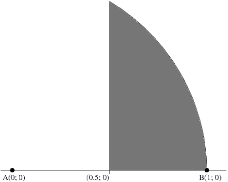
Figure 1: Initial positions of the masses: first and second are located in points A and B while third mass could be placed in any point in the gray region

problem, that is enough; should we use different masses, we have to permute the masses between A, B, and the “running” position, and use all the resulting time maps together). Initially, all three masses are at rest, but immediately after they start moving in the gravitational potential they govern. The calculation of their motion lasts until the system disrupts (at time $T_{d}$) or $T=5000$ is reached; the value for the maximal $T$ is adopted from we11_1 , where we saw that by this time $T_{d}^{-2/3}$ is clearly reached in the equal-mass case, our current research proved that as well. The disruption of the system is determined by the hyperbolicity (positivity of mechanical energy of the disrupting binary) at a distance 50 times larger than the current semi-major axis of the final binary. This way of defining is by default used in the triple code that we are using and it is quite wide-spread in studying the three-body problem in astronomy.

III Results

We have modelled over 30 million initial positions for the third mass that are evenly-distributed over the gray area in Fig. 1. The resulting $F_{a}(T_{d})$ integral distribution (the number of trajectories with the disruption time that is greater than $T_{d}$) was fitted by the power-law relation $F_{a}(T_{d})=A\times T_{d}^{\beta}$ with steps $\Delta T=10$ and $\Delta T=100$; the result is presented in the upper panel of Fig. 2: $\Delta T=10$ as the red (dark gray if grayscaled) and $\Delta T=100$ as the thick black line. The strong noise of the first curve is caused by an insufficient number of data points in each bin ($\Delta T=10$), one can easily see that the second curve is much smoother and still, it has variations. They both approach $\beta=-0.7\ldots-0.75$, which is pretty close to $\beta=-2/3$ that is expected from the first type of the Hamiltonian intermittency. On the other hand, the minimum at low $T_{d}$ points to $\beta=-3/2$ (although, it does not reach it, ending at $\beta\approx-1.06$) that is expected from the second type of the Hamiltonian intermittency, hence we investigate it further on. One note needs to be taken – with $\Delta T\gtrsim 200\ldots 400$ minimum at low $T_{d}$ could be easily missed and we believe that large $\Delta T$ was a reason why $\beta=-3/2$ was not detected in this problem earlier.

Then we fit the $F_{a}(T_{d})$ curve as a sum of both contributions $F_{a}(T_{d})=A_{1}\times T_{d}^{\beta_{1}}+A_{2}\times T_{d}^{\beta_{2}}$ and this fit gives us an excellent result: $A_{1}=3.93812\times 10^{7}\pm 5.297\times 10^{5}~{}(1.345\%)$, $A_{2}=1.2327\times 10^{9}\pm 3.707\times 10^{7}~{}(3.007\%)$, $\beta_{1}=-0.666399\pm 0.001526~{}(0.229\%)$, and $\beta_{2}=-1.501\pm 0.008454~{}(0.5633\%)$. One can see that the powers are almost exactly equal to the predicted values; in the bottom panel of Fig. 2 we presented the $F_{a}(T_{d})$ curve (thick gray), $T_{d}^{-3/2}$ contribution (dotted green), $T_{d}^{-2/3}$ (red dashed), and the sum of two contributions (thin blue). One can see that the resulting curve fits $F_{a}(T_{d})$ quite well, while $T_{d}^{-2/3}$ alone coincide with $F_{a}(T_{d})$ only starting from thousands of $T_{d}$.

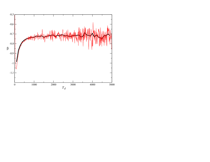
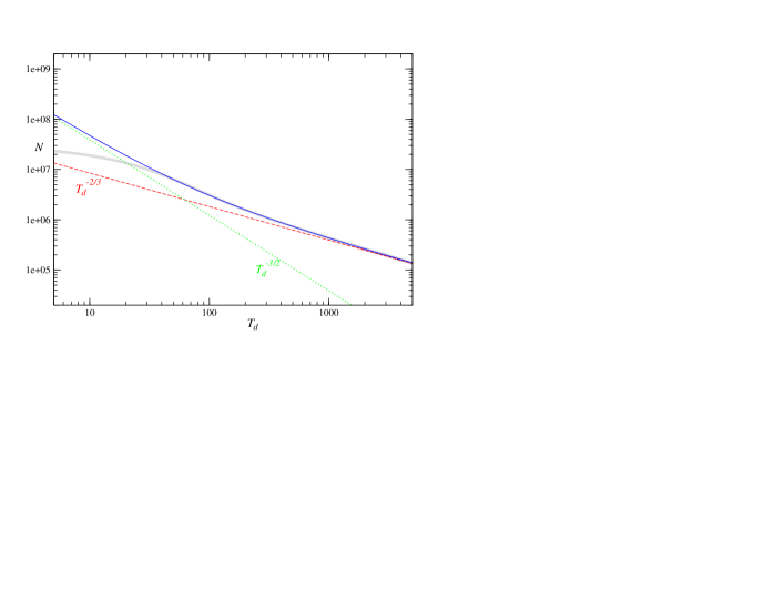
Figure 2: Upper panel: the power index of the $F_{a}(T_{d})$ power-law fit ($F_{a}(T_{d})\propto T_{d}^{\beta}$). The red (dark gray if grayscaled) curve corresponds to $\Delta T=10$ step while the thick black curve – to $\Delta T=100$. Bottom panel: best-fit of the $F_{a}(T_{d})$ curve with both contributions: the thick gray line – $F_{a}(T_{d})$, the green dotted line – $T_{d}^{-3/2}$ contribution, the red dashed line – $T_{d}^{-2/3}$, the thin blue line – the sum of two contributions. See the text for exact values of powers.

IV Conclusions

We have considered the three-body problem with unit masses that are initially at rest and demonstrated that both terms – $T_{d}^{-2/3}$ and $T_{d}^{-3/2}$ – contribute into the statistics of the disruption. The reason why $T_{d}^{-3/2}$ contribution remained undetected in the equal-mass problem is because the corresponding trajectories are stuck to the strong chaos region at low $T_{d}$. The chaotic pattern ends at the low values of $T_{d}$, so the trajectories that are stuck to its border manifest themselves strongest at low $T_{d}$ as well (though, not solely, since it is owing to the influence of $T_{d}^{-3/2}$ contribution that the power of $T_{d}^{-2/3}$ is not found exactly). Fitting the $F_{a}(T_{d})$ curve clearly demonstrated the presence of both the contributions ($T_{d}^{-2/3}$ and $T_{d}^{-3/2}$), and the powers were confirmed with great precision. We believe that the reason why the power indices found in the earlier papers on this subject (e.g.,Orlovetal2010 ) were somehow lower than the expected $-2/3$ was the interference from the $T_{d}^{-3/2}$ term. Also, high values for the maximal integration time usually lead to high values of $\Delta T$ – the size of bin to plot the distribution. If $\Delta T\gtrsim 200\ldots 400$, then the whole deep in upper panel of Fig. 2 would be inside one bin, and so it could be undetected – we believe that this was, at least, partially, a reason why both indices simultaneously remained undetected.

V Acknowledgments

The author is grateful to Alexey Toporensky and Ivan Shevchenko for fruitful discussions and to Sergey Karpov and Margarita Khabibullina for the computational help.

References

- (1) E. Strömgren, Medd. Lund. Astron. Obs. 1, 1 (1900); C. Burrau, Astron. Nachr. 195, 113 (1913).
- (2) M.J. Valtonen, Vistas Astron. 32, 23 (1988).
- (3) T. Agekian, Zh. Anosova, and V. Orlov, Astrophysics, 19, 66 (1983).
- (4) S. Mikkola and K. Tanikawa, Mon. Not. Roy. Astron. Soc. 379, L21 (2007).
- (5) I.I. Shevchenko, Phys. Rev. E 81, 066216 (2010).
- (6) V. Orlov, A. Rubinov, and I. Shevchenko, Mon. Not. Roy. Astron. Soc. 408, 1623 (2010).
- (7) F. Borgonovi, I. Guarneri, and P. Sempio, Il Nuovo Cimento B 102, 151 (1988); P. Schlagheck and A. Buchleitner, Phys. Rev. A 63, 024701 (2001).
- (8) I.I. Shevchenko and H. Scholl, Cel. Mech. Dyn. Astron. 68, 163 (1997).
- (9) G. Cristadoro and R. Ketzmerick, Phys. Rev. Lett. 100, 184101 (2008); R. Venegeroles, Phys. Rev. Lett. 102, 064101 (2009).
- (10) S. Aarseth and K. Zare, Celestial Mechanics 10, 185 (1974).
- (11) A. V. Bogomolov, S. A. Pavluchenko, and A. V. Toporensky, arXiv:1101.0399.