2mass/Hipparcos Extinctions and Distances in the Serpens – Aquila Region
IV. Error Propagation. Individual stars and mean values

1 Abstract

We estimate errors from the application of the main sequence $(H-K)_{0}\ vs.\ (J-H)_{0}$ and $(J-K)_{0}\ vs.\ M_{J}$ relations on 2mass photometry to provide stellar extinctions and distances. The error propagation on individual stars in the Serpens – Aquila star forming region is investigated. Results: errors on the $J-band$ extinction $\sigma_{A_{J}}$ are found in the range from 0.05 to 0.20 mag and peak at $\approx$0.1. For the absolute $J-band$ magnitudes the $\sigma_{M_{J}}$ range is found from 0.1 to 0.5 mag and the distribution has a pronounced maximum at $\approx$0.3 mag. Individual relative distance errors, $\sigma_{distance}/distance$, are found in the interval from 8$\%$ to 25$\%$ and peak at 15$\%$. If cloud distances are identified with the location of a local maximum of the $A_{J}(median)/distance(median)$ variation the Serpens – Aquila cloud may be at 203$\pm$7 pc. We propose that the median absolute deviation from the median of $A_{J}$ could be used as a cloud distance indicator

$Keywords$: Photometry: 2mass, Astrometry: photometric parallaxes, Error distributions: $\sigma_{A_{J}}$ , $\sigma_{M_{J}}$, $\sigma_{distance}$, $\sigma_{distance}/distance$, Molecular clouds: Serpens – Aquila, Molecular clouds: distance

2 Introduction

It is of some interest to investigate the precision of the extinctions and distances estimated from individual 2mass sources until all sky astrometry becomes available. When the photometry is precise enough 2mass data might be useful to map out 3D extinction distribution in the local Milky Way. For extinction estimates we rely on a standard $(H-K)_{0}\ vs.\ (J-H)_{0}$ relationship like Bessell and Brett [1988]. With the intrinsic colors at hand the extinction is known and distances may subsequently be derived from a calibration of $M_{J}$ in terms of $(J-K)_{0}$. The distance follows from $r(pc)=dex(0.2(J-M_{J}-A_{J}+5))$. A $M_{J}$ calibration may be established from stars common to Hipparcos and 2mass. If several stars are measuring a common interstellar feature, e.g. identified as a local maximum in the line of sight median density – distance variation, given as $A_{J}/distance$, the error of the mean distances and mean extinctions pertaining to the feature might be quite small and perhaps even comparable to those obtained from optical photometry and trigonometric parallaxes.

3 Intrinsic colors

Bessell and Brett [1988] have provided $(H-K)_{0}\ vs.\ (J-H)_{0}$ relations for main sequence and giant stars. The Bessell and Brett colors may be transformed to the 2mass system following Carpenter [2001]. New two color relations, reddening free, may be established from stars common to Hipparcos and 2mass where Hipparcos may provide distance selections more or less assuring no extinction. But such work has not been done so far. Straizys and Lazauskaite [2009] have recently presented intrinsic 2mass colors for main sequence and giant stars together with spectral classes. Standard deviations for most of their main sequence colors are given in the range from 0.02 to 0.05 mag. A comparison of Straizys and Lazauskaite [2009] main sequence to Bessell and Brett [1988] shows a good agreement. Minor deviations are only present for early type stars where Straizys and Lazauskaite’s new relation has systematically bluer $(H-K)_{0}$ colors than Bessell and Brett. Since the difference is only minor and concentrated to the earlier spectral types, which we do not use anyway, we have continued using Bessell and Brett [1988].

For the following considerations reference is made to Fig. 1. The shape of the intrinsic CCD implies two ambiguities. For a the spectral range, approximately G4 – M0, the main sequence and giant relation almost coincides. Second, the shape of the CCD signifies that beyond about M0 it becomes a problem to decide whether a star is a much reddened early type or a less reddened late type, unless additional luminosity information is available. As a consequence the first choice of reddening tracers is confined to a part of the interior of the $(H-K)_{0}\ vs.\ (J-H)_{0}$ relation in Fig. 1. We confine the observed $JHK$ sample by the upper straight line that has a slope equal to that of the reddening vector, $E_{J-H}$ / $E_{H-K}$, and intersects the main sequence where the giants branch off the main sequence. The lower confining reddening vector is introduced because the derivative of the $(H-K)_{0}\ vs.\ (J-H)_{0}$ relation is almost identical to the slope of the reddening vector implying that the intersection, $((H-K)_{0},\ (J-H)_{0})$, is undetermined.

Some stars with low or no reddening will be scattered to the blue side of the standard relation by the photometric errors. The maximum error accepted in the present note is 0.040 mag in each of the three 2mass bands. The curve to the blue of the standard relation defines the blue limit for the stars included in the sample. In order to exclude most unreddened M-type stars we impose a upper $J-H$ boundary just below the standard relation by shifting the relation by the maximum error, 0.040 mag, in J, H, and K. Stars inside the dashed ”polygon” are accepted for further study. The intrinsic colors are determined by translating a star in the accepted region of Fig. 1 along a reddening vector to intersect the standard curve. $A_{J}$ is derived from the estimated color excess $E_{J-H}$ and a standard extinction law.

4 Absolute magnitudes

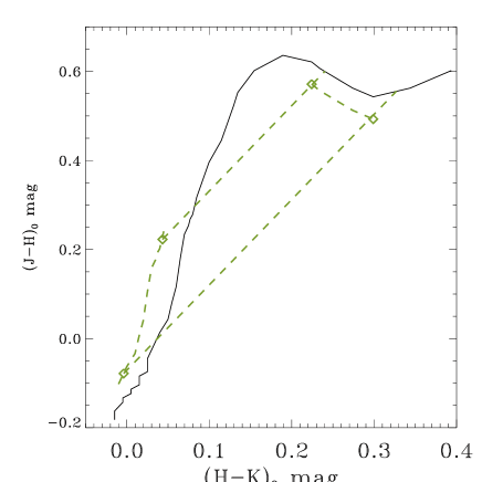
Figure 1: The dashed curve outlines the region of acceptance in the CCD. The solid curve is the Bessell-Brett [1988] standard relation for the main sequence transformed to 2mass. The upper two limitations excludes giant stars and little reddened M-type stars. The lower right limitation excludes early type stars where the slope of the standard relation approximates the reddening ratio. Stars inside the dashed curve connecting the four diamonds constitute the primary sample for which unique intrinsic colors may be estimated

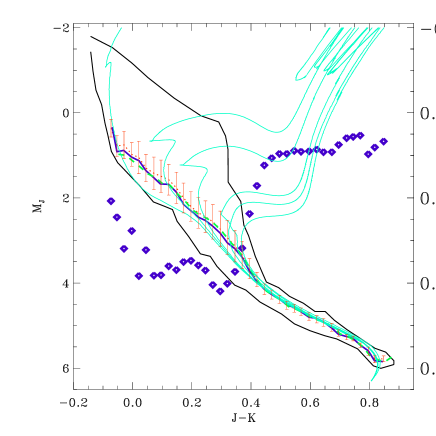
Figure 2: The closed solid curve is the confinement of the main sequence sample discussed in the text and is shown together with its resulting statistical relations calculated for 0.025 mag bins of $(J-K)$. The thick solid curve is the median given together with the standard deviation computed for 0.050 $(J-K)$ intervals. Isochrones from Cordier et al. [2007] are shown for 0.1, 0.8, 1.5, 4.0, 5.0 and 8.0 Gyr. The diamonds show $\sigma_{M_{J}}$ (right hand scale) calculated for overlapping 0.050 intervals in $(J-K)$ separated by 0.025 mag and a drop from 0.4 mag to 0.1 mag is noted where the 8 Gyr isochrone turns off the main sequence

In order to establish the main sequence $(J-K)_{0}\ vs.\ M_{J}$ relation we have extracted stars common to Hipparcos, Perryman et al. [1997], and 2mass, Cutri et al. [2003]. Two requirements are imposed on the astrometry. Precision: $\sigma_{\pi}/\pi\ <$ 10$\%$. Reddening free: $\pi\ >$ 10 mas $\Leftrightarrow$ a stellar distance $<$ 100 pc that commonly is accepted as a boundary for the reddening free local volume.

A substantial part of the Hipparcos stars has spectral and luminosity classification. From the HR diagram of the common sample it was, however, noticed that several stars have been misclassified and a large fraction of the trigonometric stars does not possess a full classification. The $M_{J}$ calibration sample is consequently not based exclusively on fully classified stars but instead the main sequence is defined by the outline shown in Fig. 2. All stars inside this boundary, and which are not known to be multiple, are accepted as main sequence stars. Median values for $(J-K)_{0}$ and $M_{J}$ are computed for 0.050 mag bins of $(J-K)_{0}$. The resulting median $(J-K)_{0}\ vs.\ M_{J}$ relation is plotted together with the errors of the means in Fig. 2. The scale on the right hand ordinate axis pertain to the errors of the mean shown as the diamonds of Fig. 2. The standard deviation results from photometric and astrometric errors, and not least from the width of the main sequence. The error of the mean is seen to vary from $\approx$0.4 to $\lesssim$0.1 mag, the better value is for stars redder than the main sequence turn off indicated by the Cordier et al. [2007] isochrones. Further details are given in Knude [2010].

5 Minor secondary sample

The stars inside the dashed confinement of Fig. 1 provide data for a first impression of the variation of extinction (e.g. $A_{J}$) vs. distance. Often an extinction rise is noticed as in Fig. 3. Some of the dwarfs inside the $(H-K)_{0}\ vs.\ (J-H)_{0}$ standard relation but above the upper reddening vector in Fig. 1 may possibly also be included by searching for stars that have extinctions and distances as indicated by the location and size of the $A_{J}$ jump. Assuming that they are $\sim$K dwarfs their absolute magitude is known from the $(J-K)_{0}\ vs.\ M_{J}$ relation. In the case of Fig. 3 distances between 150 and 250 pc and $A_{J}$ ranging from $\approx$0 to $\approx$1.2 mag outlines the parameter space where $\sim$K dwarfs are looked for. This addition to the sample might be small but the statistics for locating the $A_{J}$ jump by adding the 10 – 20 K type dwarfs, that normally result, may be improved. But we emphasize that the extinction – distance study does not depend on the inclusion of these stars.

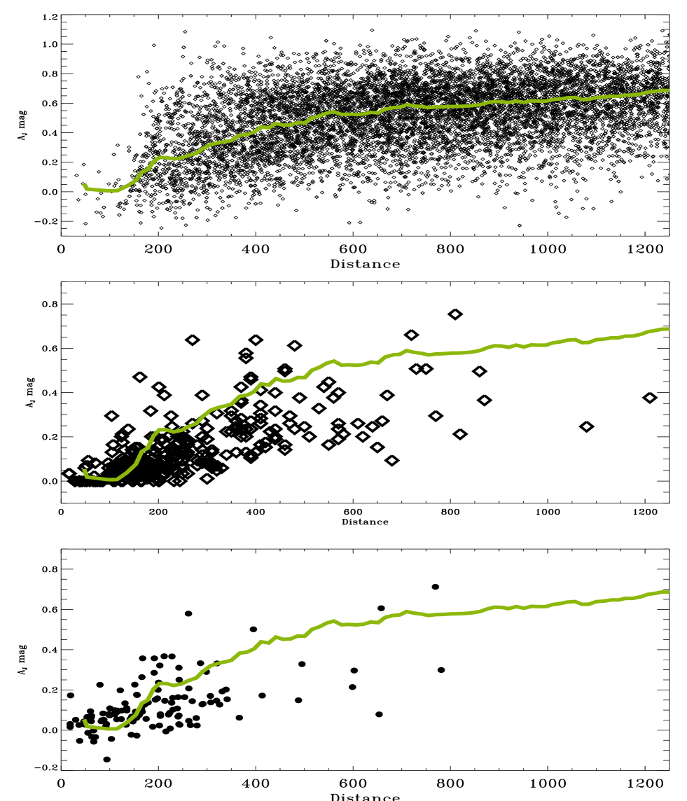
Figure 3: Upper panel Stars with $\sigma_{JHK}<$ 0.040 mag from the sky patch defined by $\alpha_{2000}$: 18^h 00^m – 18^h 30^m and $\delta_{2000}$: -3^∘ – +2^∘. Resulting distance extinction pairs. Median relation from Fig. 5 is overplotted. Central panel. Outcome of the Vilnius survey from Straizys et al. [2002]. Bottom panel. Extraction from Hipparcos. Distances are from van Leeuwen [2007], classification from Houk and Swift [1999]. For method see Knude and Høg [1998]

6 Simple error progression

For stars in the accepted parts of the CCD the intrinsic colors are estimated from translating the observed position $(H-K,J-H)$ to the intrinsic main sequence position along a reddening vector through the point. The intrinsic colors provide $(J-K)_{0}$ from which $M_{J}$ is estimated from the median relation shown in Fig. 2. The errors to be considered come from the observational errors and from the uncertainties in the slope and zero point in the reddening vector and in the two standard relations. The uncertainty in the intersection of the vector and the Bessell-Brett standard relation, approximated locally by a small line segment $(J-H)_{0}\ =\ \alpha\times(H-K)_{0}+\beta$, involves the uncertainty in the coefficients $\alpha$ and $\beta$. In a similar way we may estimate the error of the absolute magnitude $M_{J}$.

The 2mass observations, the reddening ratio and the Bessell-Brett relation result in $(H-K)_{0},(J-H)_{0}$ and therefore in $(J-K)_{0}$ and e.g. $E(J-H)$ which with the adopted reddening law is equivalent to $A_{J}$. Similarly the 2mass observations and the $(J-K)_{0}$ vs. $M_{J}$ relation provide the $M_{J}$ estimate. If $s=f(x_{i})$ represents either the full set of equations used to estimate $A_{J}$ or $M_{J}$ the formal error of $s$ follows from the progression formula:

$$\sigma_{s}^{2}=\Sigma_{i}(\frac{\partial s}{\partial_{x_{i}}}\ \sigma_{x_{i}})^{2}$$ (1)

For each star in the accepted part of the CCD we then compute $\frac{\partial s}{\partial_{x_{i}}}$ and $\sigma_{x_{i}}$ implying that derivatives must be calculated and errors of the independent parameters also must be known.

The resulting error distributions for a sample, more than 12000 stars, in the Serpens – Aquila region of the sky are shown in Fig. 4.

But before we comment on the error distributions first a little on the sampled region. The Serpens star forming region has attracted much attention over the years, e.g. Eiroa, Djupvik and Casali [2008], Straizys, Bartasiute and Cernis [2002] and Bontemps et al. [2010]. The area possesses active star forming regions and possibly contains sheets of interstellar material as well, Bontemps et al. [2010]. In order to see if the estimated parameters are not completely off the mark we have chosen to consider the rather large patch of sky studied by Straizys et al. [2002] (see their Fig. 1), $\alpha_{2000}$: 18^h 00^m – 18^h 30^m and $\delta_{2000}$: -3^∘ – +2^∘.

In this region we have extracted all stars from 2mass with $\sigma_{JHK}<$ 0.040 mag with AAA quality. After locating the stars in the region of acceptance of Fig. 1, we compute their extinction, distance and simultaneously do the error progression for the individual sources. The distance – $A_{J}$ variation itself is displayed in the upper panel of Fig. 3 and the four panels of Fig. 4 contain the distributions of $\sigma_{A_{J}},\ \sigma_{M_{J}},\ \sigma_{distance}$ and most importantly the relative distance error $\sigma_{distance}/distance$ respectively.

We may notice that despite quite a substantial number of main sequence stars are available in this part of the sky rather few are located within $\approx$200 pc. The upper left panel shows that for all these stars $A_{J}$ is estimated with an error better than $\sigma_{A_{J}}(max)\approx$ 0.2 mag corresponding to $\sigma_{A_{V}}(max)\ \lesssim$ 0.7 mag. Only three stars have a larger error. The distribution is, however, rather narrow and peaks at $\lessapprox$0.1 mag corresponding to $\sigma_{A_{V}}\ \lessapprox$ 0.35 mag.

The distribution of the absolute magnitude errors is in the upper right panel. It has a strongly peaked distribution with all stars having an almost identical error $\sigma_{M_{J}}\approx$ 0.3 mag. From Fig. 2 we know that the early type stars have the largest uncertainty $\approx$0.4 mag and that the uncertainty becomes smaller, $\approx$0.1 mag, when the turn off is approached. But most of the early type stars that may have been present in the 2mass Catalog are left out of the computations since their extinction, as mentioned, can not be derived with a sufficient accuracy. The uncertain intersection is caused by an almost parallelism of the reddening vector and the standard $(H-K)_{0}\ -\ (J-H)_{0}$ relation for this spectral range.

Combining the extinction and luminosity errors the resulting distance error distribution comes out as in the lower left panel of the Figure. Note the two logarithmic scales. The logarithmic scale is introduced on the x-axis in order to emphasize the smaller distances which have our greatest attention. The dashed curve pertains to stars with an estimated distance less than 500 pc. The total sample peaks at $\sigma_{distance}\approx$100 pc and the stars within 500 pc have errors better than $\approx$80 pc.

Finally we give the relative distance precision in the lower right of Fig. 4. The majority of stars have 0.13 $<$ $\sigma_{distance}/distance$ $<$ 0.17 and we recall that this is the estimated relative error distribution for individual stars. The distribution peaks at $\approx$0.15. An interesting point is that the relative distance error appears independent of distance when $\sigma_{JHK}<$0.040 mag. The dashed histogram are again for stars estimated to be within 500 pc. As a matter of curiosity we mention that a relative precision of 15% matches what was obtainable with photoelectric $uvby\beta$ photometry for A and F stars brighter than V$\lesssim$9 mag a generation ago, Knude [1978].

With a typical relative error of 15$\%$ on a single distance an uncertainty of $\sim$30 pc for a star at 200 pc is implied.

7 Extinction in the Serpens – Aquila region

The Serpens – Aquila region is known to contain several massive concentrations of interstellar material whose distances are under debate. Bontemps et al. [2010] quotes a range of estimated distances to the clouds and star forming regions in this part of the sky. We do not enter this discussion presently but introduce the possibilty to use the 2mass – Hipparcos calibration to estimate distances to such features. Fig. 3 displays the distance – $A_{J}$ variation as measured by individual stars. If one can show – or just assume – that different stars in a common distance interval, e.g. 150 – 180 pc are measuring extinctions pertaining to the same interstellar feature the error of the mean extinction and the mean distance - if that is relevant - may be calculated from the individual tracer errors. However, it has been a common pratice to identify an extinction discontinuity located at a fairly constant distance as caused by ”an interstellar cloud”. The solid curve in the three panels of Fig. 3 is the median distance vs. median $J-band$ extinction calculated for 30 pc bins. If the extinction jump represents a cloud its distance may be around 200 pc.

The central panel of Fig. 3 is the outcome, with $A_{V}$ converted to $A_{J}$, of the Vilnius survey of the same region for which we have extracted 2mass data and the authors identified the distance to the front of clouds in this area to 225 $\pm$55 pc , Straizys et al. [2002]. For the sake of completeness we have included what may be obtained from Hipparcos stars (HIP2: van Leeuwen [2007]) and the Michigan spectral classification Vol. 5, Houk and Swift [1999] in the same area following Knude and Høg [1998].

In all three panels the median $A_{J}$ vs. distance relation is overplotted. If the distance to the rise of the median extinction is accepted as the cloud distance the cloud seems located somewhere between 150 and 250 pc according to each of the three methods.

The upper panel of Fig. 3 shows how the median extinction varies with the median distance. Each are calculated in 30 pc bins separated by 15 pc steps. Bins within $\approx$200 pc are noticed to contain only a few stars and the error of the mean will match the individual errors rather closely. For larger distances the error of the mean extinction and distance will benefit from the larger number of stars in a given distance bin, see Table 1. In Fig. 5 the two top panels show the median variation and the corresponding errors of the mean(s). The center panel has a logarithmic distance scale to stress distances closer than $\approx$300 pc. The bottom panel of the diagram shows how the average line of sight density $A_{J}/distance\ \propto\ n_{H}$ atoms cm^-3 formed from the median values vary with distance. A density peak, statistical significant according the errors of the mean, see Table 1 for the numbers displayed on the Figure, is present at $\approx$200 pc. If we define the distance of the cloud as the distance with the maximum average line of sight density $n_{H}$ we have an indication from the $A_{J}/distance\ vs.\ distance$ diagram and even an estimate of the error on this distance: 203 $\pm$ 7 pc. The estimated error $\pm$7 pc is based on the individual errors pertaining to the 177 stars located in the 30 pc wide bin with the median distance 203 pc. In a recent report using a different method we estimated the distance to the Serpens cloud as 193 $\pm$ 13 pc, Knude [2010]. What we do not known is whether the extinctions and distances we estimate can be attributed to the star forming Serpens clouds – only that some material appears in the general direction of the clouds.

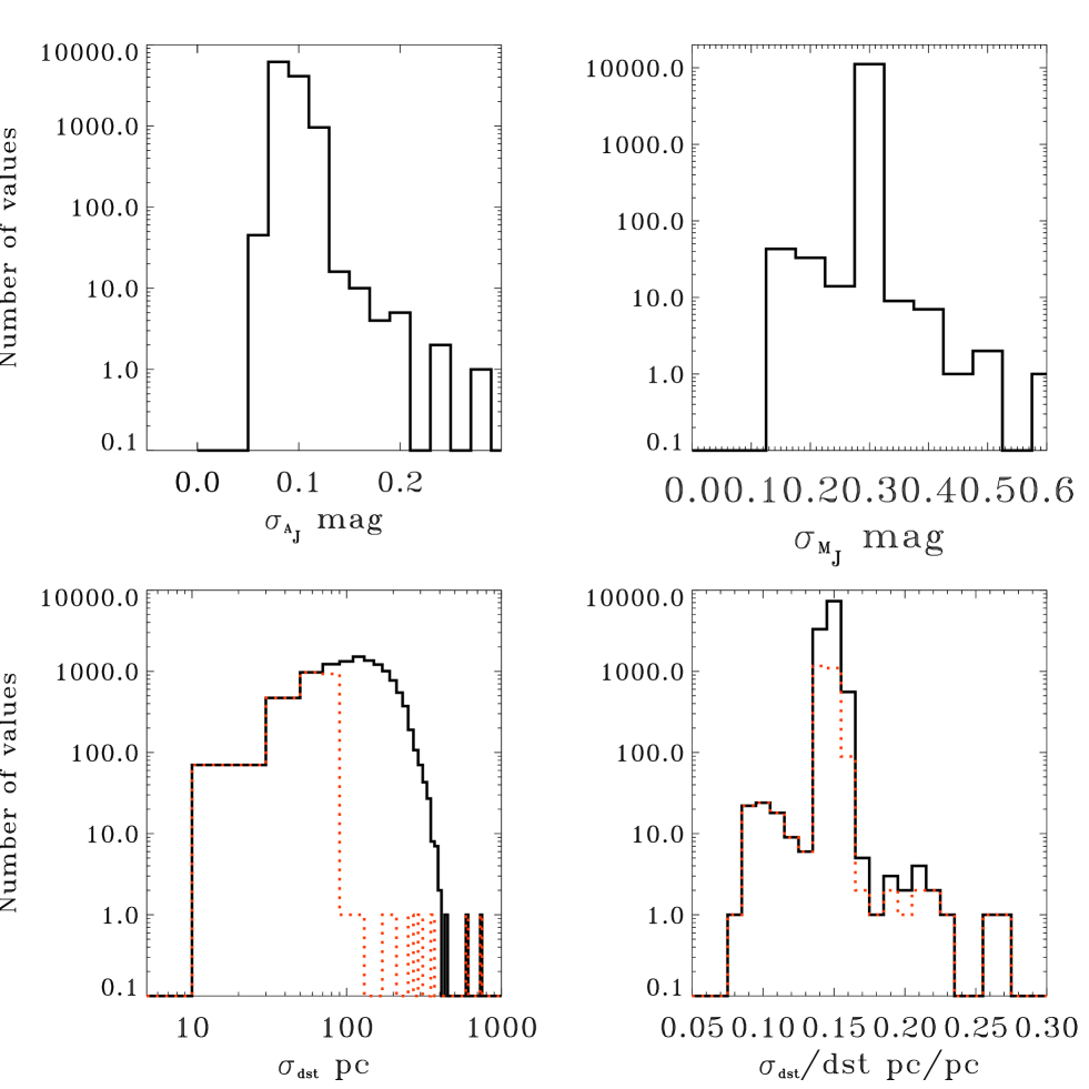
Figure 4: Distribution of errors for individual stars with $\sigma_{JHK}<$0.040 mag. Dashed curves for the two bottom diagrams pertain to stars with estimated distances less than 500 pc. The bottom right panel shows that the typical relative distance error is $\approx$15%

8 Errors in mean extinction and distance

If the extinction of all stars in a given distance range measure the same interstellar feature, which probably will have a column density variation from the cloud rim, where it approximates what is caused by the general diffuse interstellar medium, to dense interior cores, we may use median values to indicate a distance estimate to this feature. In Knude [2010] it was suggested that $\overline{H-K}_{reseau}$ contours, where the reseau size was defined from the requirement that a reseau should hold 100 stars on the average, was useful to define cloud outlines. Note that because our sample is only selected from the region of acceptance of Fig. 1 large extinctions are not measured: $A_{J}(max)$ $\lesssim$1.5 mag. As the upper panel of Fig. 3 shows the $A_{J}$ increases around 200 pc. Noting that the relative distance error is about 15$\%$ we have bined the stars in 30 pc intervals. In Table 1 we show values for the first 15 distance intervals and results are plotted in Fig. 5. The upper panel displays the variation of the medians: $distance(median)\ vs.\ A_{J}(median)$. For each distance bin the error of the mean for both variables are also displayed. The central panel has a logarithmic scale to emphasize the nearer distances but is otherwise identical to the upper panel. The lower panel indicates that cloud distances possibly may be identified by a local maximum in the line of sight average density $A_{J}/distance$ mag/pc $\propto$  $n_{H}$ atoms/cm³. Errors of distance as well as the average line of sight density are indicated.

Table 1: Median distance and extinction in the $J-band$ band together with errors of the mean. The mean and median are calculated for 30 pc distance bins. Column 5 indicates the number of stars in a bin. Column 6 is $A_{J}(median)/distance(median)$ in mag/pc and Column 7 is the error of this ratio based on the errors of Column 2 and 4. Exclusively from stars in the region of acceptance and the minor set of secondary K dwarfs all with $\sigma_{JHK}<$0.040 mag

Distance	Error	$A_{J}$	Error	#	$A_{J}/distance$	$\sigma(A_{J}/distance)$
pc	pc	mag	mag		mag/pc	mag/pc
102.0	45.5	0.0061	0.0410	6	5.98039e-05	0.000403061
109.7	34.0	0.0061	0.0303	11	5.56062e-05	0.000277036
112.2	31.7	0.0010	0.0287	12	8.91266e-06	0.000256118
135.0	18.6	0.0354	0.0192	26	0.000262222	0.000146937
151.8	15.6	0.0429	0.0163	38	0.000282609	0.000111483
166.3	13.1	0.1157	0.0127	62	0.000695731	9.46005e-05
179.2	8.6	0.1661	0.0092	113	0.000926897	6.83839e-05
191.4	7.6	0.2317	0.0081	143	0.00121055	6.42917e-05
203.3	6.7	0.2547	0.0073	177	0.00125283	5.51005e-05
217.0	6.3	0.2627	0.0067	206	0.00121060	4.74362e-05
231.4	6.6	0.2583	0.0068	204	0.00111625	4.35682e-05
246.7	6.3	0.2688	0.0065	221	0.00108958	3.86119e-05
262.0	6.2	0.3008	0.0063	239	0.00114809	3.66818e-05
277.1	6.1	0.3192	0.0062	246	0.00115211	3.41028e-05
290.9	6.3	0.3317	0.0061	256	0.00114025	3.25962e-05

Figure 5: Upper panel. Median of distances and extinctions $A_{J}$ calculated for 30 pc bins. The median points are plotted together with the error of the mean also for 30 pc bins. Middle panel. Same as Upper panel but on a logarithmic distance scale to emphasize nearby bins. 15 nearest bins are tabulated in Table 1. Bottom panel Line of sight average density $A_{J}/distance$ with errors

8.1 Another Cloud Distance Indicator?

Traditionally the location of a cloud has been identified by the presence of an extinction jump at a rather well defined distance and the distance(s) of the nearest star(s) showing the extinction rise have been used to estimate a lower limit to the cloud distance. Star forming clouds at least are expected to show a large variation in column densities and one could imagine that a cloud do have a distribution of deviations from the median column density different from that pertaining to stars at a given distance and situated outside clouds. A possible statistics able to show the signature of a cloud could be the Median Absolute Deviation from the median of $A_{J}$, MAD($A_{J}$). In Fig. 6 we show a preliminary presentation of the possible use of MAD($A_{J}$). In the lower ight panel is shown the variation of MAD($A_{J}$) with median distance and the near coincidence of an extremum of MAD($A_{J}$) and the peak in the line of sight average density $A_{J}(median)$/$Distance(median)$ is noticed.

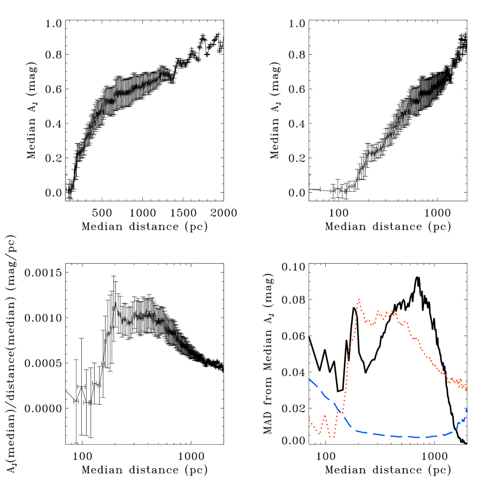
Figure 6: Set of diagrams including MAD: Median Absolute Deviation from the median, considered to be a rather robust statistics. Upper left. Median curve with error bars indicating the Median Absolute Deviation of distance and extinction. Upper right. Same as Upper left but on a logarithmic distance scale. Lower left. Average density $A_{J}(median)$/$Distance(median)$. MAD of both coordinates is plotted. Lower right. MAD($A_{J})$ vs. median distance is plotted as the solid curve. The dotted curve is a scaled version of the average density (multiplied by 70). The dashed curve is the run of the error of the mean extinction vs. distance. From Fig. 4 we recall that the typical error of $A_{J}$ is $\lesssim$0.1 mag. The near coincidence of MAD($A_{J})$ and the peak of the average line of sight density is noticed

9 Acknowledgements

This publication makes use of data products from the Two Micron All Sky Survey, which is a joint project of the University of Massachusetts and the Infrared Processing and Analysis Center/California Institute of Technology, funded by the National Aeronautics and Space Administration and the National Science Foundation. This research has made use of the SIMBAD database, operated at CDS, Strasbourg, France.

References

- [1988] Bessell, M.S., Brett, J.M. 1988, PASP 100, 1134
- [2010] Bontemps et al. 2010, A&A 518, L85
- [2001] Carpenter, J.M. 2001, AJ 121, 2851
- [2007] Cordier, D., Pietrini, A., Cassisi, S., Salaris, M. 2007, AJ 133, 468
- [2003] Cutrie, R.M. et al. 2003, The 2MASS All Sky Catalog of Point Sources
- [2008] Eiroa, C., Djupvik, A.A., Casali, M.M. 2008, Handbook of Starforming Regions: The Southern Sky. ASP Monograph Publications Vol. 5, p. 693. Edited by Bo Reipurth
- [1999] Houk, N., Swift, C. 1999, The Michigan Catalogue of two dimensional spetraltypes of the HD Stars; Vol. 5
- [1978] Knude, J. 1978, A&AS 33, 347
- [2010] Knude, J. 2010 arXiv:1006.3676v1
- [1998] Knude, J., Høg, E. 1998, A & A, 338, 897
- [1997] Perryman, M.A.C., Lindegren, L., Kovalewsky, J., Høg, E., Bastian, U., et al. 1997, AA 323, L49
- [2002] Straiys, V., Bartasiute, S., ernis, 2002 Baltic Astron. 11, 417
- [2009] Straiys, V., Lazauskaite, R. 2009, Baltic Astron. 18, 19
- [2007] van Leeuwen, F. 2007, A&A 474, 653