How to take turns: the fly’s way to encode and decode rotational information
Ingrid M. Esteves, Nelson M. Fernandes and Roland Köberle
DipteraLab, Inst. de Física de São Carlos, University of São Paulo,
13560-970 São Carlos, SP, Brasil
Contact e-mail: rk@if.sc.usp.br
Running head: Neural code of spike trains.
Keywords: neural code, spike trains, information theory
ABSTRACT
Sensory systems take continuously varying stimuli as their input and encode features relevant for the organism’s survival into a sequence of action potentials - spike trains. The full dynamic range of complex dynamical inputs has to be compressed into a set of discrete spike times and the question, facing any sensory system, arises: which features of the stimulus are thereby encoded and how does the animal decode them to recover its external sensory world?

Here we study this issue for the two motion-sensitive H1 neurons of the fly’s optical system, which are sensitive to horizontal velocity stimuli, each neuron responding to oppositely pointing preferred directions. They constitute an efficient detector for rotations of the fly’s body about a vertical axis. Surprisingly the spike trains $\rho_{B}(t)$ generated by an empoverished stimulus $S_{B}(t)$, containing just the instants when the of velocity $S(t)$ reverses its direction, convey the same amount of global (Shannon) information as spike trains $\rho(t)$ generated by the complete stimulus $S(t)$. This amount of information is just enough to encode the instants of velocity reversal. Yet this suffices to give the motor system just one, yet vital order: go left or right, turning the H1 neurons into efficient analog-to-digital converters. Furthermore also probability distributions computed from $\rho(t)$ and $\rho_{B}(t)$ are identical. Still there are regions in the spike trains following velocity reversals, 80 msec long and containing about 3-6 msec long spike intervals, where detailed stimulus properties are encoded. We suggest a decoding scheme - how to reconstruct the stimulus from the spike train, which is fast and works in real time.

Introduction
All living organisms rely on the sensory nervous system to quickly and reliably extract relevant information about a changing external environment. E.g. the visual system receives time-continuous optical flow patterns and generates a set of discrete identical pulses, called action potentials or spikes. This analog-to-digital conversion means that only a small fraction of relevant stimulus properties is actually encoded in the spike train and a lot of effort has been expended in finding out just which and how [20, 35, 15, 34, 16, 18, 17, 32, 27, 30, 14]. Debates have been going on for decades over the way and means employed by the organism to effect this dimensional reduction[24, 25, 26, 33, 23, 29, 4] without losing essential information. Although these studies have revealed a wealth of interesting properties, a much more direct approach would be to investigate the animal’s performance to a stimulus, manufactured to contain only relevant features. Once these have been successfully guessed and appropriately tested, we need a decoding algorithm to reconstruct the stimulus from the spike train. It should work in real time to be available to the animal, using only data which are presumably held in a memory.

To explore these issues we recorded spikes from the two motion sensitive H1 neurons - one for each compound eye - of the fly Chrysomya megacephala. Each H1 neuron is sensitive to horizontally moving stimuli, being excited by back-to-front motion and inhibited by the oppositely moving scenery. They measure rotational velocities of the fly’s body around a vertical axis [12]. In our experiments the fly sees a rigid pattern moving with horizontal velocity $S(t)$ either on a Tektronix monitor or on a large translucent screen - see Methods for details. From $S(t)$ we manufacture an empoverished version $S_{B}(t)$, which tells the fly only which way the scenery is rotating: either to the left or to the right. $S_{B}(t)$ generates spike trains $\rho_{B}(t)$, which are indistiguishable from the ones $\rho(t)$ generated by $S(t)$, as far as global averages over the whole experiment are concerned. Yet we discover specific local regions on a time scale of $~{}50-100$ msec, where the responses $\rho(t)$ and $\rho_{B}(t)$ do differ. Thus the encoding and decoding process should occur in a multilayered fashion, involving several time scales.

Generating the same response raster with boxed stimuli
Consider one H1 neuron and let its excitatory stimuli be positive ($S(t)>0$) and inhibitory negative ($S(t)<0$). Instants when the stimulus velocity reverses sign correspond to the zero-crossings of the stimulus $S(t)$. We now discretize our continuous stimulus $S(t)$ and generate a discrete boxed version $S_{B}(t)$, assigning different values to positive and negative velocities:

$$S_{B}(t)=\left\{\begin{array}[]{c}S_{0},{\sf if}S(t)\geq 0\\ -S_{0},{\sf if}S(t)<0.\end{array}\right.$$

The constant $S_{0}$ will be chosen so that $S(t)$ and $S_{B}(t)$ have the same variance We emphasize that $S(t)$ and $S_{B}(t)$ have the same zero-crossings.

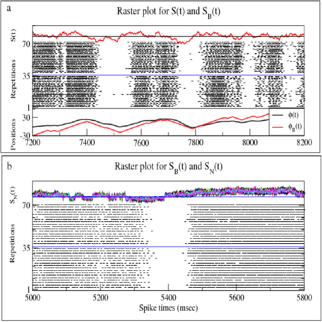
Figure 1: Rasterplots of spikes generated by $S(t)$ and its boxed and noisy versions. a: Section of rasterplots for spikes generated by $S(t)$ and $S_{B}(t)$. $S(t)$ is a gaussian velocity signal with correlation time $\tau=60$ msec, the raster-time running from $7200$ to $8200$ msec Repetitions $1:35$ are due to $S(t)$, whereas $36:70$ are due its boxed versions $S_{B}(t)$. The bottom graph shows the actual screen positions $\phi(t)$ and $\phi_{B}(t)$ (deg) as seen by the fly for $S(t)$ and $S_{B}(t)$. Experiment: Tektronix, $\tau=$ 60 msec. b: Section of rasterplots for spikes generated by $S_{B}(t)$ and noise-added stimuli $S_{N}(t)$. Repetitions $1:35$ are due to $S_{B}(t)$, whereas $36:70$ are due noise-added gaussian stimuli $S_{N}(t)$. On top we show the superposition of all stimuli $S_{N}(t)$. Experiment: Natural, $\tau=200$ msec, $f=0.5$.

We subject the fly alternately to stimuli $S(t)$ and $S_{B}(t)$, each being $10$ sec long. They are repeatedly shown the fly, the odd/even repetitions being due to $S(t)$/$S_{B}(t)$ respectively. From the responses of the H1 neuron we construct a raster, each dot representing a single spike. In Fig.1a we show a section of this raster plot with $35$ repetitions for each stimulus, where we collected the responses due to $S(t)$ below repetition $35$ and the ones due to $S_{B}(t)$ above. The result is completely unexpected: visually there is no significant difference between repetitions. Notice that the plots of the screen positions $\phi(t)$ and $\phi_{B}(t)$ emphasize, that the fly does not even view the same picture, when subjected to $S(t)$ and $S_{B}(t)$. Apparently the fly’s H1 sensory system does not pay attention to any details of stimulus $S(t)$, which are lost in $S_{B}(t)$.

To further explore this striking fact, we generate a whole set of stimuli $S_{N}(t)$ adding a certain amount of random noise to $S_{B}(t)$, but always preserving the zero-crossings. The noise added is measured by the ratio $f\equiv\sigma(S-S_{N})/\sigma(S_{N})$, where $\sigma$ is the stimulus variance. Subjecting the fly to the set $S_{B}(t),S_{N}(t)$, we obtain the raster of Fig.1b. Repetitions $1:35$ are due to $S_{B}(t)$ and the the remaining ones due to $S_{N}(t)$, the noise being different for each repetition $36:70$. Again no difference can be seen between the two sets. For a quantitative test, we compute the interval histograms due to $\rho_{N}(t)$ and $\rho_{B}(t)$, shown in Fig.2: the are the same. Additionally all the rank-ordered word distributions of $\rho_{N}(t)$ and $\rho_{B}(t)$ look identical. In the insets of Fig.2 we plot these distributions for binary words of lengths $L=5,8$. This astonishing identity also hold for longer words, although the word lables for $L>7$ are then not all identical.

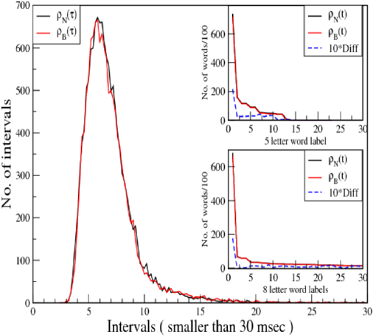
Figure 2: Interval histograms for noise added stimuli. Compare the interval histograms generated by stimuli $S_{N}(t)$ and $S_{B}(t)$. The black (red) curve is the interval histogram of $\rho_{N}(t)$ ($\rho_{B}(t)$). Upper inset: Five letter word distributions for $\rho_{N}(t)$ and $\rho_{B}(t)$. The time axis was discretized into $2$ msec wide bins. The presence of a spike in each bin was represented by 1 and the absence by 0. Each binary word is a sequence of five 1’s or 0’s and we have $2^{5}=32$ possible word labels. We plot the rank-ordered word distribution for $\rho_{N}(t)$ and $\rho_{B}(t)$, using identical labels for both histograms. Their difference, upscaled by $10$, is shown as the dashed (blue) curve. Lower inset: Same as upper inset for the first thirty eight letter words, but now the word labels $W(i)$ and $W_{B}(i)$ for $\rho_{N}(t)$ and $\rho_{B}(t)$ are not all identical. E. g. $W(j)=W_{B}(j),j=1,2,3,4$, but $W(5)=W_{B}(6),W(6)=W_{B}(5)$. Experiment: Tektronix, $\tau=60$ msec, $f=0.5$.

This equivalence holds true for a host of global statistical averages. Examples, which have been used a lot to characterize neural responses, are the Shannon mutual informations (MI) $I[\rho|S]$, $I[\rho_{B}|S_{B}]$, which the spike trains $\rho(t)$, $\rho_{B}(t)$ convey about the stimuli $S(t)$, $S_{B}(t)$ respectively. Using the direct method of Ref. [28], we plot in Fig.3a the total entropies $E[\rho]$,$E[\rho_{B}]$ of the spike trains and the entropies conditioned on their stimuli $E[\rho|S]$,$E[\rho_{B}|S_{B}]$. Informations are given by $I[S|\rho]=E[\rho]-E[\rho|S]$, $I[S_{B}|\rho_{B}]=E[\rho_{B}]-E[\rho_{B}|S_{B}]$. Notice that $\rho(t)$ conveys the same amount of MI about the total stimulus $S(t)$ as $\rho_{B}(t)$ conveys about the boxed stimulus $S_{B}(t)$. Thus, as far as the MI is concerned, $\rho(t)$ ignores all the features in $S(t)$, which are absent in $S_{B}(t)$, paying attention only to whether the scenery moves left or right. Since the entropy of $S_{B}(t)$ is about ten times smaller than $S(t)$’s, this amounts to a huge entropy reduction with a concomitant increase in coding efficency $e$, defined as the ratio of MI divided by stimulus entropy.

The boxed stimulus $S_{B}(t)$ is characterized by its zero-crossings, half of them being from negative to positive stimulus values (upcrossings) and the other half the opposite. The information to locate all the upcrossings $I_{upzc}$ is about equal to $I[\rho|S]$, as shown in Fig.3a. It is therefore consistent to assume that one H1 neuron extracts enough information to locate the up-zero-crossings. Recording from both H1 neurons[9], we obtain an efficiency $e=0.42$, again just enough to locate all (up and down) zero-crossings of the stimulus .

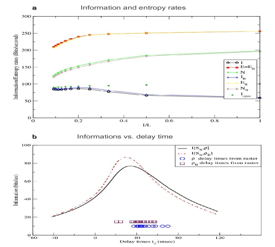
Figure 3: Information and entropy rates. a: Information and Entropy rates vs. 1/wordlength. Spike times were discretized at $2$ msec and the cell’s responses were represented as binary words of length $L$ bins. The word-entropies $E\equiv E[\rho]$ and $E_{B}\equiv E[\rho_{B}]$ are identical. $N=E[\rho|S]$ and $N_{B}=E[\rho_{B}|S_{B}]$ - the entropies, which the distributions of words convey about the respective stimuli - and $I\equiv I[\rho|S]$, $I_{B}\equiv I[\rho_{B}|S_{B}]$ coincide within errors. Errors are $\sim 10\%$. $I_{upzc}$ is the information-rate to locate up-zero-crossings. Experiment: Tektronix, $\tau=60$ msec. b: Delay times from $I[S_{B},\rho]$, $I[S_{B},\rho_{B}]$ and raster plots. Squares, circles are delay times of common ZC’s for $\rho$, $\rho_{B}$ extracted directly from raster plots. To compute $I[S_{B},\rho]$ and $I[S_{B},\rho_{B}]$ time is binned into $2$ msec. To obtain the required probability distributions $pr[S_{B}|\rho_{B}](t_{d})$, $pr[S_{B}|\rho](t_{d})$ we proceed as follows. We sample the spike-train distribution $\rho_{B}(t)$ through a window four bins long, obtaining a set of binary words $W_{B}$ with their multplicity $m_{B}$ and their occurrences $t_{1}$. For each word $W_{B}$ we sample $m_{B}$ stimulus words $W_{S_{B}}$ of size four, but at instants $t_{1}-t_{d}$. Varying $t_{d}$ we compute $pr[W_{S_{B}}|W_{B}](t_{d})$ to obtain $I[S_{B},\rho_{B}]$. We repeat the procedure for $\rho(t)$. Experiment: Tektronix, $\tau=160$ msec.

Two coding regions after zero-crossings
Up to now we have endeavored to show that the H1 neuron reponds equally to $S(t)$ and its boxed version, but there could still be subtle differences, if we look more closely. To unravel differences between $\rho(t)$ and $\rho_{B}(t)$ we select prominent zero-crossings (ZC). These are instants, when the velocities $S(t)$, $S_{B}(t)$ change from negative to positive values leading to well defined onsets of spiking activity- see Methods for details. We compute spike rates after each ZC for a time interval of $400$ msec, shown in Fig.4. We observe that there are in fact two coding regions I and II, following the first spike after ZC’s. Region I spans a time $T_{1}\sim 80$ msec. Here the rate for $\rho_{B}(t)$ is larger than the $\rho_{B}(t)$’s, reflecting the stronger response to sharper onset of positive stimuli. This is followed by region II, where the rates for $\rho(t)$ and $\rho_{B}(t)$ are the same.

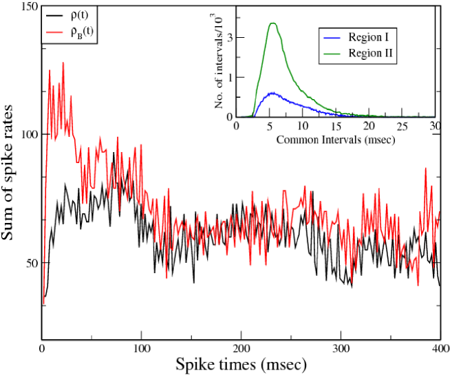
Figure 4: Spike rates after ZC. Sum of spike rates of $\rho(t)$ (black) and $\rho_{B}(t)$ (red) summed over $71$ ZC’s. The time axis is discretized into $2$ msec bins and translated so that the first spike after ZC occurs at $t=0$. $\rho_{B}(t)$’s spike rate is always larger and merges with $\rho(t)$’s after $\sim 80$ msec. Experiment: Tektronix, $\tau=400$ msec, $f=0.5$. Inset: Histograms for intervals ($\leq 30$ msec) common to $\rho(t)$ and $\rho_{B}(t)$ for regions I and II, using all experiments.

To take a closer look at regions I and II, we compute in each region intervals common to $\rho(t)$ and $\rho_{B}(t)$, accumulating data ($\sim 50.000$ data points) from ZC’s of all experiments. The histograms of these intervals are shown in the inset of Fig.4. Both histograms peak around $6$ msec, but their shape is different. This could encode the ”YES, adjust to turns ” information, which the H1 neurons should extract from the stimulus and relay to the motor system. Since the variances of $S(t)$ and $S_{B}(t)$ are the same, the spike trains should encode this and presumably other ensemble properties in Region II[8]. A more detailed investigation of regions I and II could allow the extraction of the precise interval structure associated with the turning command. Due to the - on average - sharper onset of the boxed stimulus $S_{B}(t)$ after ZC, the spiking precision of the first and second spike after all ZC’s is always better for $\rho_{B}$ as shown in Table 1. This underscores the sensibility of the H1 neuron to discontinuities in the stimulus.

$\tau$ (msec)	$\overline{\sigma}^{(1)}$ (msec)	$\overline{\sigma}_{B}^{(1)}$ (msec)	$\overline{\sigma}^{(2)}$ (msec)	$\overline{\sigma}_{B}^{(2)}$ (msec)	$N^{\tau}$	N${}_{B}^{\tau}$
10	4.35	3.37	3.63	3.34	70	70
30	4.97	3.83	4.81	3.73	71	75
80	5.81	4.19	5.75	4.60	39	41
100	4.66	4.34	4.67	4.56	48	44
200	7.23	5.42	6.43	5.53	29	25

Table 1: Mean variance of first and second spike after all ZC’s for stimuli $S$ and $S_{B}$ vs. correlation lengths $\tau$. $\overline{\sigma}^{(1)}$ ($\overline{\sigma}_{B}^{(1)}$): Mean variance of 1^st spike for $\rho(t)$ ($\rho_{B}(t)$); $\overline{\sigma}^{(2)}$ ($\overline{\sigma}_{B}^{(2)}$): Mean variance of 2^nd spike for $\rho(t)$ ($\rho_{B}(t)$). For each stimulus $S$ we find all ZC’s and compute the variances $\sigma$ of the 1^st and 2^nd spike after each ZC. The mean $\overline{\sigma}$ is taken over the three types of experiments (Natural, Bars, Tektronix), using a total of $N^{\tau}$($N^{\tau}_{B}$) zero-crossings for $\rho(t)$ ($\rho_{B}(t)$) respectively.

A further boxed vs. complete stimulus dependent property are the delays - the times it takes the fly to generate the first spike after ZC. These times exhibit a pronounced dependence on the stimulus history as shown Fig.3b. Here we plot delay times, extracted directly from raster plots, for $\rho(t)$ as circles and for $\rho{{}_{B}}(t)$ as squares. For comparision we also compute mean delay times $t_{d}$ extracted from the MI’s ( $I[S_{B}|\rho],I[S_{B}|\rho_{B}]$ ), which the spike trains $\rho(t_{1})$ and $\rho_{B}(t_{1})$ convey about the boxed stimulus $S_{B}(t)$. When plotted as a function of $t_{d}$ they show a pronounced peak, which provides a mean-information-delay-time. As we move off the peaks, the correlation between stimulus and spike-train vanishes and - although not shown in the figure - all information rates actually do vanish for large $|t_{d}|$. Notice that the peak values are identical to the MI obtained by the direct method of Ref. [28]. In all cases the neuron responds faster by $\sim 10$ msec to the boxed stimuli, emphasizing again the systems sensitivity to sharp stimulus variations. newline

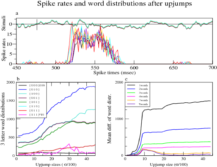
Figure 5: a. Spike rates (poststimulus time histograms) after upjump for jumpsizes $n*\sigma/100,n=1,2,..,45$. The peak between $500$ and $600$ msec is due to the zero-crossings at $t\sim 475$ msec - see stimuli on top. Its structure clearly depends on stimulus variance, as revealed by the two plots below. b: 3 letter word distributions $W^{(3)}_{i}(n)$ in the peak plotted against $n$. The word distribution for no spikes ($[000]$) is downscaled by a factor of $100$ and the one for all occupied by spikes ($[111]$) is upscaled by a factor of $10$. Binsize is $2$ msec. c: Mean of the word-distribution difference $W_{i}(n)-W_{i}(1)$ for word-lengths $1,2,3,4,7,8$. Experiment: Tektronix, $\tau=200$ msec.

Sensitivity of H1 to temporal discontinuities
If one of the foremost aims of the H1 neurons is the extraction of temporal discontinuities from the optical flow, in order to respond preferentially only to these, the fly has to decide on a threshold: how much stimuli have to rise above the background for them to be classified as discontinuities?

Let us measure discontinuities by changes in stimulus variance $\delta\sigma$, defining $f\equiv\delta\sigma/\sigma$. To study this situation, often stimuli are chosen, which are piecewise constant. Since the variance of a constant equals zero, $f=\infty$ and the fly obviously interprets this as a discontinuity, even if $\delta\sigma$ is small. To simulate a more realistic situation, we expose the fly to a series of random gaussian stimuli $S_{n}(t)$ with correlation times $\tau=200$ msec and variances $\sigma_{n}$. They are generated from a common stimulus $S_{0}(t)$ with standard deviation $\sigma_{0}=7$ deg, by upscaling its standard deviation as $\sigma_{n}=n*\sigma_{0}/100,n=1,2,3,..,45$. Fig.5a shows the spike rates generated by the stimuli on top. The zero-crossing for $n=1$ occurs at $t_{1}=475$ msec and for $n=45$ at $t_{45}=478$ msec with intermediate values for the other n-values. These zero-crossing initiate the large spike-rate at $t\sim 510$ msec. To expose the structure of this peak’s spike patterns, we compute the distributions for all 3 letter words $W^{(3)}_{i}(n),n=1,2,3,..,45,i=1,2,..,8=2^{3}$ in the peak, shown in Fig.5b. The distributions change for upjump sizes $n>3$. To emphasize this, we subtract the distributions for the smallest upjump to get $dW^{(3)}_{i}(n)=W^{(3)}_{i}(n)-W^{(3)}_{i}(1)$ and take their mean $\overline{dW^{(3)}_{i}}=<dW^{(3)}_{i}(n)>_{n}$. In Fig.5c we show these means for word-sizes $1,2,3,4,7,8$, which clearly show a steep rise starting at the $3\%$ upjump. A distributional encoding of the variance can be seen: words of all lengths contribute to small ($n\leq 15$) upjumps, whereas large upjumps are encoded into words of length $\leq 4$. Thus under our experimental conditions the threshold for detection is a $\sim 3\%$ change in variance.

Discussion
An efficient representation of the sensory input is one of the main requirements to be satisfied by a neural code[4]. Shannon’s mutual information between stimulus and spike train is often used to asses this efficiency. Our results show that this measure is too coarse, since it is unable to distinguish the complete stimulus from its boxed version. We find in fact that the mutual information is only sufficient to encode the zero-crossings of the stimulus. Yet a closer look reveals a multilayered scheme[8, 3] of which we observe two layers, suggesting the following scenario. In a region $80$ msec long after spiking onset following zero-crossings we observe spike patterns, about $6$ msec long, which encode turning commands, whereas stimulus ensemble properties, like stimulus variance, are encoded on time scales longer than $80$ msec. If variance changes together with zero-crossings, the fly’s detection time is much shorter: from the data of Fig.5 we extract a time-scale of $\sim 37$ msec for a change in stimulus variance of $\geq 3\%$.

Once we know that the spike train carries just enough information to encode the position of all the zero-crossings, what does this tell us about the decoding problem: how does the fly recover the stimulus from H1’s spike train? This information allows the extraction of the zero-crossings (or reconstruction of the boxed stimulus $S_{B}(t)$ up to a scale factor) rather straightforewardly for stimulus correlation times $\tau>200$ msec: select a spike train for some repetition in a raster and search it for $10$ msec long gaps, followed by 3-4 spikes less than $\sim 10$ msec apart - this will locate up-zero-crossings $ZC_{sp}$ . They coincide with all the up-zero-crossings $ZC_{r}$ obtained from the spike rate. Peaks signalling onset of spiking activity and locating $ZC_{r}$, are defined as spike rates larger the 60% of the repetition number and no preceeding spiking activity for $20$ msec. This definition of $ZC_{r}$ excludes zero-crossings too small to be relevant for the fly and extracts only the important ones. An identical procedure applied to the responses of the contra-lateral H1 neuron locates the down-zero-crossings. For correlation times smaller than $200$ msec more elaborate schemes have to be adopted.

Since not all zero-crossings are equivalent it stands to reason, that more information is allocated to the important ones. It is thus probable, using the spike patterns stored in region I, that more than $S_{B}(t)$ can be recovered from a spike train. Since we know that the H1 neuron has acces to the mean and variance of the stimulus[5], a fast local reconstruction procedure could be accomplished in two (or more) stages. First the important zero-crossings would be extracted from the spike trains, the other encoded properties supplying the scale factor required to reconstruct $S_{B}(t)$. In the second stage more stimulus details could be included using e. g. the usual Volterra series reconstruction[22, 10], although this requires the knowledge of stimulus-spike correlation functions like $<S(t_{1})\rho(t_{2})>$, whose update at the milisecond time scale is problematic.

We have only analyzed the output of H1 neurons and suggested a way to extract the specific sequence of spikes, which would relay the turning command to the motor neurons. The fly uses also mechanosensory organs, gyroscopes using Coriolis forces, to detect fast self-rotations[21, 6]. These are the halteres, beating at the same frequency as the wings. The visual and mechanosensory inputs are then fused to obtain a more robust estimate of the stimulus[13, 11]. Therefore we have to keep in mind, that there are many other sensory pathways, which respond to stimulus details not detected by the H1 neurons.

Methods
Experimental Setup and Preparation
Immobilized flies were shown a rigidly moving scenery, while action potentials - spikes - were recorded extracellularly from H1 neurons. We used two experimental setups: Tektronix and Slide. In the Tektronix setup, the fly views vertical bar patterns on a Tektronix 608 monitor, whose update-rate was $500$ Hz, so that the bar pattern moved by $\delta x=v(t)$ every $2$ ms[1, 2]. In the Slide setup the fly views a large ( 60 cm x 40 cm ) translucent convex cylindrical screen, a slide being projected on the concave side via a simple optical system containing two mirrors. These are analogically controlled by linear motors, cannibalized from hard disk controllers. They move the slide’s projection horizontally across the screen[7]. This setup produces a continously moving image, but its performance is limited by mechanical inertia and fatigue. We therefore use it only for stimuli with correlation time $\tau\geq 60$ msec. The slide we use shows either a natural scenery or a random vertical bar pattern - called ”Natural” or ”Bars” in the text. Although we recorded simultaneously from both H1 neurons, for simplicity we only use one neuron recordings and select a subset of these for our figures. All our conclusion hold for two neuron recordings[9].
All experiments were repeated involving about $30$ flies.
Stimulus
The velocity stimuli $v(t)$ were taken from Gaussian distributions with exponentially decaying correlation functions $\sim exp(-t/\tau)$.
Searching for zero crossings
When the stimulus crosses from negative to positive values, one of the H1 neurons typically starts to generate spikes after a delay time of $\sim 40$ msec. To locate a well defined peak of spiking activity, we compute the spike rate - or the poststimulus time histogram - summing for each time bin the occurencies of spikes over all repetitions in the raster. To locate peaks, we require a spike rate larger than half the number of repetitions in a small window of a couple of msec. Prominent instants are to be preceeded by no spiking activity for at least $100$ msec and we require peaks to be present in both spike trains $\rho(t)$ and $\rho_{B}(t)$. Additionally no new peak is allowed for the next $400$ msec.

Acknowledgments
We thank I. Zuccoloto, L. O. B. Almeida and J. F. W. Slaets for help with the experiments. NMF was supported by a FAPESP and IME by a CNPq fellowship. The laboratory was partially funded by FAPESP grant 0203565-4. We thank Altera Corporation for their University program and Scilab for its excellent software.

References

- [1] L. Almeida.,Desenvolvimento de instrumentação eletronica para estudos de codificações neurais no duto óptico em moscas. Master’s thesis, Univ. of São Paulo, Brazil, 2010. Available at: http://www.teses.usp.br/teses/disponiveis/76/76132/tde-29032007-105503/en.php.
- [2] L. O. B. Almeida, J. F. W. Slaets, and R. Köberle. VSImg: A high frame rate bitmap based display system for neuroscience research. Neurocomputing, 2011.
- [3] M. S. Baptista, C. Grebogi, and R. Köberle. Dynamically multilayered visual system of the multifractal fly. Physical Review Letters, 97:178102–1–178102–4, 2006.
- [4] H. Barlow. Possible principles underlying the transfomations of sensory images. In W. Rosenblith, editor, Sensory Communication, pages 217–234. MIT Press, Cambridge, MA, 1961.
- [5] N. Brenner, W. Bialek, and R. de Ruyter van Steveninck. Adaptive rescaling maximizes information transmission. Neuron, 26:695–702, 2001.
- [6] M. H. Dickinson. Haltere-mediated equilibrium reflexes of the fruit fly Drosophila melanogaster. Philosophical Transactions of the Royal Society, 354:903–916, 1999.
- [7] I. M. Esteves. Gerador de estimulos visuais para pesquisar o sistema visual da mosca. Master’s thesis, Univ. of São Paulo, Brazil, 2010. Available at: www.teses.usp.br/teses/disponiveis/76/76131/tde-04102010-171911/en.php.
- [8] A. L. Fairhall, G. D. Lewen, W. Bialek, and R. R. van Steveninck. Efficiency and ambiguity in an adaptive neural code. Nature, 412(6849):787–792, 2001.
- [9] N. M. Fernandes. Acuidade visual e codificação neural de mosca Chrysomya megacephala. PhD thesis, Univ. of São Paulo, Brazil, 2010. Available at: www.teses.usp.br/teses/disponiveis/76/76131/tde-25032010-161256/en.php.
- [10] N. M. Fernandes, B. D. L. Pinto, L. O. B. Almeida, J. F. W. Slaets, and R. Köberle. Recording from two neurons: second order stimulus reconstruction from spike trains. Neural Computation, 186(4):399–407, 2009.
- [11] Jessica L. Fox, Adrienne L. Fairhall, and Thomas L. Daniel. Encoding properties of haltere neurons enable motion feature detection in a biological gyroscope. Proceedings of the National Academy of Sciences, 107(8):3840–3845, 2010.
- [12] K. Hausen. Monokulare und Binokulare Bewegungsauswertung in der Lobula Platte der Fliege. Verh. Dtsch. Zool. Ges., pages 49–70, 1981.
- [13] S. J. Houston and H. G. Krapp. Nonlinear integration of visual and haltere inputs in fly neck motor neurons. J. Neuroscience, 29(42):13097–13105, 2009.
- [14] P. Kara, P. Reinagel, and R. C. Reid. Low response variability in simultaneously recorded retinal, thalamic and cortical neurons. Neuron, 27:635–646, 2000.
- [15] J. Keat, P. Reinagel, R. C. Reid, and M. Meister. Predicting every spike: a model for the responses of visual neurons. Neuron, 30:803–17, 2001.
- [16] S. Laughlin. Visual motion: Dendritic integration makes sense of the world. Current Biology, 9:R15–R17, 1999.
- [17] S. B. Laughlin. Energy as a constraint on the coding and processing of sensory information. Current opinion in neurobiology, 11:475–480, 2001.
- [18] G. D. Lewen, W. Bialek, and R. R. van Steveninck. Neural coding of naturalistic motion stimuli. Network-Computation in Neural Systems, 12(3):317–329, 2001.
- [19] Jr. Logan. Information in the zero crossings of bandpass signals. Bell Systems Technical Journal, 56:487 – 510, 1974.
- [20] I. Nemenman, G. D. Lewen, W. Bialek, and R. R. van Steveninck. Neural coding of natural stimuli: Information at sub-millisecond resolution. Plos Computational Biology, 4:e1000025, 2008.
- [21] J. W. S. Pringle. The gyroscopic mechanism of the halteres of diptera. Philosophical Transactions of the Royal Society, 233:347–385, 1999.
- [22] F. Rieke, D. Warland, R. R. van Steveninck, and W. Bialek. Spikes -exploring the neural code. MIT Press, Cambridge, USA, 1997.
- [23] S. T. Roweis and L. K. Saul. Nonlinear dimensionality reduction by locally linear embedding. Science, 290:2323–2229, 2000.
- [24] A. B. Saleem, H. G. Krapp, and S. R. Schultz. Receptive field characterization by spike-triggered independent component analysis. Journal of Vision, 8(13):1–16, 2008.
- [25] T. Sharpee and W. Bialek. Neural decision boundaries for maximal information transmission. Plos ONE, 2(7):646, 2007.
- [26] T. Sharpee, N.C. Rust, and W. Bialek. Analyzing neural responses to natural signals: Maximally informative dimensions. Neural Computation, 16:223–250, 2002.
- [27] D. Smyth, B.Willmore, G.E.Baker, I.D. Thompson, and J.D. Tolhurst. The receptive-field organization of simple cells in primary visual cortex of ferrets under natural scene stimulation. J. Neurosci., 23:4746–4759, 2003.
- [28] S. P. Strong, R. Köberle, R. R. van Steveninck, and W. Bialek. Entropy and information in neural spike trains. Physical Review Letters, 80(1):197–200, 1998.
- [29] J. B. Tenenbaum, V. da Silva, and J. C. Langford. A global geometric framework for nonlinear dimensionality reduction. Science, 290:2319–2323, 2000.
- [30] F. E. Theunissen, K. Sen, and A.Doupe. Spectral-temporal receptive fields of nonlinear auditory neurons obtained using natural sounds. J. Neurosci., 20:2315–2331, 2000.
- [31] Y. V. Venkatesh. Hermite polynomials for signal reconstruction from zero-crossings. IEEE Proceedings-I, 139:587–, 1992.
- [32] N. J. Vickers, T. A. Christensen, T. Baker, and K. G. Hildebrand. Odour-plume dynamics influence the brain’s olfactory code. Nature, 410:466–470, 2001.
- [33] T. von der Twer and D. I. A. McLeod. Optimal nonlinear codes for the perception of natural colours. Network: Comput. Neural Syst., 12:395–401, 2001.
- [34] M. Wainwright. Visual adaptation as optimal information transmission. Vision Research, 39:3860–3974, 1999.
- [35] B. D. Wright, K. Sen, W. Bialek, and A. J. Doupe. Spike timing and the coding of naturalistic sounds in a central auditory area of songbirds. In T.G. Dietterich, S. Becker, and Z. Ghahramani, editors, Advances in Neural Information Processing, volume 14, pages 309–316. MIT Press, Cambridge, MA, 2002.