Non-Gaussian velocity distributions
– The effect on virial mass estimates of galaxy groups

Abstract

We present a study of 9 galaxy groups with evidence for non-Gaussianity in their velocity distributions out to 4$R_{200}$. This sample is taken from 57 groups selected from the 2PIGG catalog of galaxy groups. Statistical analysis indicates that non-Gaussian groups have masses significantly higher than Gaussian groups. We also have found that all non-Gaussian systems seem to be composed of multiple velocity modes. Besides, our results indicate that multimodal groups should be considered as a set of individual units with their own properties. In particular, we have found that the mass distribution of such units are similar to that of Gaussian groups. Our results reinforce the idea of non-Gaussian systems as complex structures in the phase space, likely corresponding to secondary infall aggregations at a stage before virialization. The understanding of these objects is relevant for cosmological studies using groups and clusters through the mass function evolution.

1 Introduction

Groups of galaxies contain most of galaxies in the Universe and are the link between individual galaxies and large-scale structures (e.g., Huchra & Geller 1982; Geller & Huchra 1983; Nolthenius & White 1987; Ramella et al. 1989). The dissipationless evolution of these systems is dominated by gravity. Interactions over a relaxation time tend to distribute the velocities of the galaxy members in a Gaussian distribution (e.g. Bird & Beers 1993). Thus, a way to access the dynamical stage of galaxy groups is to study their velocity distributions. Evolved systems are supposed to have Gaussian velocity distributions, while those with deviations from normality are understood as less evolved systems. Hou et al. (2009) have examined three goodness-of-fit tests (Anderson-Darling, Kolmogorov and $\chi^{2}$ tests) to find which statistical tool is best able to distinguish between relaxed and non-relaxed galaxy groups. Using Monte Carlo simulations and a sample of groups selected from the CNOC2, they found that the Anderson-Darling (AD) test is far more reliable at detecting real departures from normality in small samples. Their results show that Gaussian and non-Gaussian groups present distinct velocity dispersion profiles, suggesting that discrimination of groups according to their velocity distributions may be a promising way to access the dynamics of galaxy systems.

Recently, Ribeiro, Lopes & Trevisan (2010) extended up this kind of analysis to the outermost edge of groups to probe regions where galaxy systems might not be in dynamical equilibrium. They found significant segregation effects after splitting up the sample in Gaussian and non-Gaussian systems. In the present work, we try to further understand the nature of non-Gaussian groups. In particular, we investigate the problem of mass estimation for this class of objects, and their behaviour in the phase space. The paper is organized as follows: in Section 2 we present data and methodology; Section 3 contains a statistical analysis with sample tests and multimodality diagnostics for non-Gaussian groups; finally, in Section 4 we summarize and discuss our findings.

2 Data and Methodology

2.1 2PIGG sample

We use a subset of the 2PIGG catalog, corresponding to groups located in areas of at least 80% redshift coverage in 2dF data out to 10 times the radius of the systems, roughly estimated from the projected harmonic mean (Eke et al. 2004). The idea of working with such large areas is to probe the effect of secondary infall onto groups. Members and interlopers were redefined after the identification of gaps in the redshift distribution according to the technique described by Lopes et al. (2009). Finally, a virial analysis is perfomed to estimate the groups’ properties. See details in Lopes et al. (2009a); Ribeiro et al. (2009); and Ribeiro, Lopes & Trevisan (2010). We have classified the groups after applying the AD test to their galaxy velocity distributions (see Hou et al. 2009 for a good description of the test). This is done for different distances, producing the following ratios of non-Gaussian groups: 6% ($R\leq 1R_{200}$), 9% ($R\leq 2R_{200}$), and 16% ($R\leq 3R_{200}$ and $R\leq 4R_{200}$). We assume this latter ratio (equivalent to 9 systems) as the correct if one desires to extending up the analysis to the regions where galaxy groups might not be in dynamical equilibrium. Approximately 90% of all galaxies in the sample have distances $\leq 4R_{200}$. This is the natural cutoff in space we have made in this work. Some properties of galaxy groups are presented in Table 1, where non-Gaussian groups are identified with an asterisk. Cosmology is defined by $\Omega_{m}$ = 0.3, $\Omega_{\lambda}$ = 0.7, and $H_{0}=100~{}h~{}{\rm km~{}s^{-1}Mpc^{-1}}$ Distance-dependent quantities are calculated using $h=0.7$.

Table 1: Main properties of groups

Group	$R_{200}$ (Mpc)	$M_{200}$ ($10^{14}~{}M_{\sun}$)	$\sigma$ (km/s)	$N_{memb}$	$N_{200}$
55	0.689	0.400	173.203	16	9
60	0.664	0.359	120.395	41	12
84	1.025	1.326	224.715	54	10
91	0.848	0.754	164.293	34	4
102∗	1.550	4.602	433.218	32	8
130	0.999	1.245	240.908	43	11
138∗	1.271	2.578	348.885	74	14
139	0.997	1.250	235.740	39	12
169	0.765	0.573	225.212	9	4
177∗	1.178	2.100	336.309	45	14
179∗	1.663	5.897	471.352	23	10
181	1.247	2.488	393.379	29	12
188	0.514	0.174	153.714	8	2
191	0.707	0.456	268.517	14	10
197	0.897	0.930	297.903	13	7
204	1.493	4.333	473.813	33	12
209	0.680	0.407	132.095	15	4
222	1.243	2.494	315.355	22	8
236	1.258	2.575	331.308	19	7
271	0.968	1.093	240.691	41	15
326	0.648	0.333	167.764	21	7
352∗	1.656	5.618	496.694	31	13
353	0.873	0.826	220.025	34	12
374	0.902	0.919	217.038	21	10
377	0.480	0.138	132.466	13	5
387	0.649	0.345	125.308	32	5
398	0.781	0.601	182.800	29	12
399	0.917	0.973	183.397	34	7
409	1.078	1.583	251.071	64	11
410	0.847	0.769	199.465	42	8
428	1.201	2.191	342.440	26	14
435	0.606	0.283	123.549	23	4
444	0.820	0.697	244.491	13	7
447∗	1.169	2.032	296.919	37	6
453	0.827	0.720	271.840	17	10
455	1.588	5.088	454.227	65	15
456	0.319	0.041	58.138	16	3
458	0.642	0.336	115.674	18	4
466	1.507	4.381	554.511	23	13
471	1.128	1.832	399.078	22	14
475∗	1.152	1.952	294.413	28	6
479	0.806	0.671	160.887	17	6
480	0.923	1.006	272.058	23	12
482	0.663	0.373	202.903	17	9
484	1.099	1.702	268.116	32	7
485	1.679	6.076	559.140	29	18
488	1.220	2.334	326.566	42	12
489	0.872	0.852	188.283	30	6
493	1.170	2.061	323.268	30	10
504	1.319	2.985	429.207	30	13
505∗	1.176	2.111	336.804	20	7
507∗	1.459	4.036	436.498	27	11
513	0.724	0.495	178.637	19	6
515	1.117	1.817	298.220	30	13
519	0.808	0.689	207.011	17	4
525	0.495	0.158	108.230	9	3
536	2.003	10.576	676.902	45	24

3 Non-Gaussianity and Mass

3.1 The mass bias

We consider the two sample statistical problem for the Gaussian (G) and NG (non-Gaussian) subsamples. We choose the mass resulting from the virial analysis as the property to illustrate the comparison between the subsamples. Both Kolmogorov-Smirnov (KS) and Cramer-von Mises (CvM) tests reject the hypothesis that the NG subsample is distributed as the G subsample, with p-values 0.00001 and 0.00029, respectively. For these tests, we have used 1000 bootstrap replicas of each subsample to alleviate the small sample effect. The result indicates an inconsistency between the mass distributions of G and NG groups. This could represent a real physical difference or, more probably, an indication of a significant bias to higher masses in NG groups. The median mass for this subsample is $\langle M_{200}^{NG}\rangle=2.57\times 10^{14}~{}M_{\sun}$, while it is $\langle M_{200}^{G}\rangle=8.85\times 10^{13}~{}M_{\sun}$ for the G subsample, thus $\langle M_{200}^{NG}\rangle$ is larger by a factor of $\sim 2.9$. In the following, we investigate this mass bias looking for features in the velocity distributions of galaxy groups.

3.2 Exploring non-Gaussianity

The shape of velocity distributions may reveal a signature of the dynamical stage of galaxy groups. For instance, systems with heavier tails than predicted by a normal parent distribution may be contamined by interlopers. Otherwise, systems with lighter tails than a normal may be multimodal, consisting of overlapping distinct populations (e.g. Bird & Beers 1993). We now try to understand the mass bias in the NG subsample by studying non-Gaussianity in the velocity distributions. Since we have carefully removed interlopers from each field (see Section 2.1; and Lopes et al. 2009a), we consider here that the most probable cause of normality deviations in our sample is due to a superposition of modes in the phase space (e.g. Diemand & Kuhlen 2008). Visual inspection of radial velocity histograms of NG systems suggests that multipeaks really happen in most cases (see Figure 1).

We statistically check multimodality by assuming the velocity distributions as Gaussian mixtures with unknown number of components. We use the Dirichlet Process mixture (DPM) model to study the velocity distributions. The DPM model is a Bayesian nonparametric methodology that relies on Markov Chain Monte Carlo (MCMC) simulations for exploring mixture models with an unknown number of components (Diebolt & Robert 1994). It was first formalised in Ferguson (1973) for general Bayesian statistical modeling. The DPM is a distribution over $k$-dimensional discrete distributions, so each draw from a Dirichlet process is itself a distribution. Here, we assume that a galaxy group is a set of $k$ components, $\sum_{i=1}^{k}\pi_{i}f(y|\theta_{i})$, with galaxy velocities distributed according to Gaussian distributions with mean and variance unknown. In this framework, the numbers $\pi_{i}$ are the mixture coefficients that are drawn from a Dirichlet distribution. In the DPM model, the actual number of components $k$ used to model data is not fixed, and can be automatically inferred from data using the usual Bayesian posterior inference framework. See Neal (2000) for a survey of MCMC inference procedures for DPM models.

In this work, we find $k$ using the R language and environment (R Develoment Core Team) under the dpmixsim library (da Silva 2009). The code implements mixture models with normal structure (conjugate normal-normal DPM model). First, it finds the coefficients $\pi_{i}$, and then separates the components of the mixture, according to the most probable values of $\pi_{i}$, in the distributional space, leading to a partition of this space into regions (da Silva 2009). The results can be visually analysed by plotting the estimated kernel densities for the MCMC chains. In Figure 2, we show the DPM diagnostics for each group, that is, the deblended modes in the velocity distributions. We have found the following number of modes per group: 4/102, 3/138, 3/177, 2/179, 5/352, 3/447, 2/475, 3/505, 3/507. Therefore, all non-Gaussian groups in our sample are multimodal (reaching a total of 28 modes) according to the DPM analysis. Unfortunately, we cannot compute the physical properties of 13 modes, due to intrinsic scattering in velocity data (and/or to the smallness of the modes – those with less than 4 members). The properties of the other 15 modes are presented in Table 2.

3.3 The mass bias revisited

Figure 1: Histograms of radial velocities for all non-Gaussian groups.

Now, we perform again the statistical tests, comparing the distribution of mass in NG and G with the new sample (see Figure 3). First, we compare the NG subsample and the sample of modes (M). Both KS and CvM tests reject the hypothesis that M is distributed as NG, with p=0.0211 and p=0.0189, respectively. Then, we compare G and M. Now, the tests accept the hypothesis that M is distributed as G, with p=0.4875 and p=0.4695. Hence, the distribution of the modes deblended from non-Gaussian groups are themselves mass distributed as Gaussian groups. Also, the median mass of the M sample is $\langle M_{200}^{M}\rangle=1.33\times 10^{14}~{}M_{\sun}$, a value larger than $\langle M_{200}^{G}\rangle$ only by a factor $\sim 1.5$ (before deblending groups the factor was $\sim$ 2.9). This consistency between G and M objects indicate that non-Gaussian groups are a set of smaller systems, probably forming an aggregate out of equilibrium. Indeed, groups are the link between galaxies and larger structures. Thus, our results suggest we are witnessing secondary infall (the secondary modes) onto a previously formed (or still forming) galaxy system (the principal mode). Naturally, we cannot discard the possibility of NG groups being unbound systems of smaller groups seen in projection, although the properties of the independent modes are quite similar to those found in physically bound groups.

Figure 2: DPM density probability decomposition. Velocities are rescaled to the [0,1] interval.

Table 2: Main properties of individual modes

Mode	$R_{200}$ (Mpc)	$M_{200}$ ($10^{14}~{}M_{\sun}$)	$\sigma$ (km/s)	$N_{200}$
102a	1.077	1.549	337.482	21
102b	0.728	0.477	153.372	4
138a	1.550	4.677	498.927	35
177a	1.249	2.481	369.569	11
177b	1.212	2.289	362.462	14
179a	1.326	3.001	336.265	8
352a	0.487	0.142	158.571	6
352b	0.941	1.033	218.210	6
352c	0.697	0.416	208.670	3
352d	0.558	0.213	181.206	5
447a	1.016	1.330	240.437	3
447b	1.192	2.155	441.382	5
475a	1.500	4.308	470.516	19
475b	2.345	16.347	829.977	10
505a	0.928	1.040	228.411	3

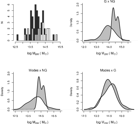
Figure 3: Histograms for Gaussian (dark gray) and non-Gaussian (white) groups. Histogram of modes is plotted in light gray. Density probability comparison among systems. Intersections areas are in white.

4 Discussion

We have classified galaxy systems after applying the AD normality test to their velocity distributions up to the outermost edge of the groups. The purpose was to to investigate regions where galaxy systems might not be in dynamical equilibrium. We have studied 57 galaxy groups selected from the 2PIGG catalog (Eke et al. 2004) using 2dF data out to $4R_{200}$. This means we probe galaxy distributions near to the turnaround radius, thus probably taking into account all members in the infall pattern around the groups (e.g. Rines & Diaferio 2006; Cupani, Mezzetti & Mardirossian 2008). The corresponding velocity fields depend on the local density of matter. High density regions should drive the formation of virialized objects, whereas low density environments are more likely to present streaming motions, i.e., galaxies falling toward larger potential wells constantly increasing the amplitude of their clustering strength (e.g. Diaferio & Geller 1997).

We have found that 84% of the sample is composed of systems with Gaussian velocity distributions. These systems could result from the collapse and virialization of high density regions with not significant secondary infall. They could be groups surrounded by well organized infalling motions, possibly reaching virialization at larger radii. Theoretically, in regions outside $R_{200}$, we should apply the non-stationary Jeans formalism, leading us to the virial theorem with some correction terms. These are due to the infall velocity gradient along the radial coordinate and to the acceleration of the mass accretion process (see Cupani 2008). Their contribution is likely to be generally negligible in the halo core where the matter is set to virial equilibrium and to become significant in the halo outskirts where the matter is still accreting (see e.g. Cupani, Mezzetti & Mardirossian 2008). However, a slow and well organized infalling motion to the center of the groups could diminish the importance of the correction terms, i.e., the systems could be in a quasi-stationary state outside $R_{200}$. The high fraction of groups immersed in such surroundings suggests that ordered infalling motion around galaxy groups might happen quite frequently in the Universe.

In any case, Gaussian groups can be considered as dynamically more evolved systems (see Ribeiro, Lopes & Trevisan 2010). The remaining 16% of the sample is composed of non-Gaussian groups. We found that these sytems have masses significantly larger than Gaussian groups. This biasing effect in virial masses is basically due to the higher velocity dispersions in NG groups. Ribeiro, Lopes & Trevisan (2010) found that NG groups have rising velocity dispersion profiles. A similar result was found by Hou et al. (2009). Rising velocity dispersion profiles could be related to the higher fraction of blue galaxies in the outskirts of some galaxy systems (see Ribeiro, Lopes & Trevisan 2010; and Popesso et al. 2007).

At the same time, the NG subsample is composed of multipeak objects, identified by the DPM model analysis applied to the velocity space. These results indicate that secondary infall might be biasing the mass estimates of these groups. Thus, the NG systems could result from the collapse of less dense regions with significant secondary infall input. Contrary to Gaussian groups, the surroundings of NG systems do not seem to be in a quasi-stationary state. They are dynamically complex. Actually, we have found these groups can be modelled as assemblies of smaller units. After deblending groups into a number of individual modes, we have verified that the mass distribution of these objects is consistent with that of Gaussian groups, suggesting that each unit is probably a galaxy group itself, a system formed during the streaming motion toward the potential wells of the field.

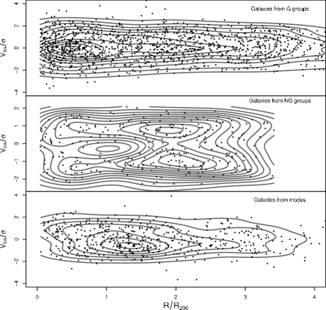
Figure 4: Phase space diagrams for a typical Gaussian (upper box), non-Gaussian (middle box) and modes (lower box) systems. Density contours indicate galaxy concentration across the diagrams. Distances to the center of the systems are normalized by $R_{200}$. Radial velocities are subtracted from the median velocity and divided by the velocity dispersion of the groups.

Our results reinforce the idea of NG systems as complex structures in the phase space out to $4R_{200}$. This scenario is illustrated in Figure 4, where we show the stacked G and NG groups, and the stacked modes. Galaxies in these composite groups have distances and line-of-sight velocities with respect to the centers normalized by $R_{200}$ and $\sigma$, respectively. In the upper box, we present the G stacked group. Note that galaxies are extensively concentrated in the phase space diagram, with a single density peak near to 0.5$R_{200}$, revealing a well organized system around this point. Also, note that the density peak has $V_{los}/\sigma\approx 0$. Contour density lines suggest that ordered shells of matter are moving toward the center. A different result is found for the NG stacked group. In the middle box of Figure 4, we see a less concentrated galaxy distribution, with less tight density contour levels, presenting a density peak slightly larger than $R_{200}$, and two additional peaks, around 2$R_{200}$, possibly interacting with the central mode. The additional peaks are not aligned at $V_{los}/\sigma\approx 0$, suggesting a less symmetrical galaxy distribution in the phase space. These features suggest that non-Gaussian systems are distinct, and dynamically younger than Gaussian groups, which agrees well with the results of Ribeiro, Lopes & Trevisan (2010). Also in Figure 4, we present the modes stacked system in the lower box. Similar to the Gaussian case, we have a single peak in the phase space, near to 1.5$R_{200}$. Galaxy distribution however is still less symmetrical than in Gaussian groups, with the peak not aligned at $V_{los}/\sigma\approx 0$. This suggests that, although more organized than NG systems, modes are probabably dynamically distinct and younger than Gaussian groups as well.

Our work points out the importance of studying NG systems both to possibly correct their mass estimates and multiplicity functions, as well as to better understand galaxy clustering at group scale. Understanding of these objects is also relevant for cosmological studies using groups and clusters through the evolution of the mass function (Voit 2005). Using systems with overestimated properties may lead to a larger scatter in the mass calibration (Lopes et al. 2009b) and could also affect the mass function estimate (Voit 2005).

References

- [] Bird, C. & Beers, T., 1993, AJ, 105, 1596
- [] Cupani, G., 2008, PhD Thesis, University of Trieste
- [] Cupani, G., Mezzetti, M. & Mardirossian, F., 2008, MNRAS, 390, 645
- [] da Silva, A.F., 2009, Comput. Methods Programs Biomed., 94, 1
- [] Diaferio, A. & Geller, M., 1997, ApJ, 481, 633
- [] Diebolt, J. & Robert C.P., 1994, Journal of the Royal Statistical Society, Series B, 56,363
- [] Diemand, J. & Kuhlen, M., 2008, ApJ, 680, L25
- [] Eke, V.R. et al. (2dfGRS Team), 2004, MNRAS, 348, 866
- [] Ferguson, T.S., 1973, Annals of Statistics, 1, 209
- [] Geller, M.J. and Huchra, J.P., 1983, ApJS, 52, 61
- [] Hou, A., Parker, L., Harris, W. & Wilman, D.J., 2009, ApJ, 702, 1199
- [] Huchra, J.P. and Geller, M.J., 1982, ApJ, 257, 423
- [] Lopes P.A.A., de Carvalho R.R., Kohl-Moreira J.L., Jones C., 2009a, MNRAS, 392, 135
- [] Lopes P.A.A.,de Carvalho R.R., Kohl-Moreira J.L., Jones C., 2009b MNRAS, 399, 2201
- [] Neal, R.M., 2000, Journal of Computational and Graphical Statistics, 9, 249
- [] Nolthenius, R. and White, S.D.M., 1987, MNRAS, 225, 505
- [] Popesso, P., Biviano, A., Böringer, H. & Romaniello, M., 2007, A&A, 461, 397
- [] Ramella, M., Geller, M. & Huchra, J.P., 1989, ApJ, 344, 57
- [] Ribeiro, A.L.B., Trevisan, M., Lopes, P.A.A & Schilling, A.C., 2009, A&A, 505, 521
- [] Ribeiro, A.L.B., Lopes, P.A.A & Trevisan, M., 2010, MNRAS, 409, L124
- [] Rines, K. & Diaferio, A., 2006, AJ, 132, 1275
- [] Voit, G. M. 2005, Rev. Mod. Phys., 77, 207