Subcritical percolation with a line of defects

Abstract

We consider the Bernoulli bond percolation process $\mathbb{P}_{p,p^{\prime}}$ on the nearest-neighbor edges of $\mathbb{Z}^{d}$, which are open independently with probability $p<p_{c}$, except for those lying on the first coordinate axis, for which this probability is $p^{\prime}$. Define

$$\xi_{p,p^{\prime}}:=-\lim_{n\to\infty}n^{-1}\log\mathbb{P}_{p,p^{\prime}}(0\leftrightarrow n\mathbf{e}_{1})$$

and $\xi_{p}:=\xi_{p,p}$. We show that there exists $p_{c}^{\prime}=p_{c}^{\prime}(p,d)$ such that $\xi_{p,p^{\prime}}=\xi_{p}$ if $p^{\prime}<p_{c}^{\prime}$ and $\xi_{p,p^{\prime}}<\xi_{p}$ if $p^{\prime}>p_{c}^{\prime}$. Moreover, $p_{c}^{\prime}(p,2)=p_{c}^{\prime}(p,3)=p$, and $p_{c}^{\prime}(p,d)>p$ for $d\geq 4$. We also analyze the behavior of $\xi_{p}-\xi_{p,p^{\prime}}$ as $p^{\prime}\downarrow p_{c}^{\prime}$ in dimensions $d=2,3$. Finally, we prove that when $p^{\prime}>p_{c}^{\prime}$, the following purely exponential asymptotics holds:

$$\mathbb{P}_{p,p^{\prime}}(0\leftrightarrow n\mathbf{e}_{1})=\psi_{d}e^{-\xi_{p,p^{\prime}}n}\bigl{(}1+o(1)\bigr{)}$$

for some constant $\psi_{d}=\psi_{d}(p,p^{\prime})$, uniformly for large values of $n$. This work gives the first results on the rigorous analysis of pinning-type problems, that go beyond the effective models and don’t rely on exact computations.

, and

t1Supported in part by the Swiss National Science Foundation.

t2Supported by the Israeli Science Foundation Grant 817/09.

1 Introduction and results

We consider bond percolation on $\mathsf{E}^{d}$, the set of nearest-neighbor edges of $\mathbb{Z}^{d}$, $d\geq 2$. Let $\mathcal{L}\subset\mathsf{E}^{d}$ be the set of all edges that lie on the first coordinate axis $\{s\mathbf{e}_{1},s\in\mathbb{R}\}$, where $\mathbf{e}_{1}$ denotes the unit vector $(1,0,\ldots,0)\in\mathbb{R}^{d}$. Let $\mathbb{P}_{p,p^{\prime}}$ be the probability measure on sets of configurations of edges $\omega\in\{0,1\}^{\mathsf{E}^{d}}$, under which each edge $e\in\mathsf{E}^{d}$ is open independently with probability

$$\mathbb{P}_{p,p^{\prime}}\bigl{(}\omega(e)=1\bigr{)}=\cases{p,&\quad if $e\in\mathsf{E}^{d}\setminus\mathcal{L}\equiv\mathcal{L}^{c}$,\cr p^{\prime},&\quad if $e\in\mathcal{L}$.}$$ (1)

When $p^{\prime}=p$, we write $\mathbb{P}_{p}$ instead of $\mathbb{P}_{p,p}$, and the model coincides with ordinary homogeneous Bernoulli edge percolation, whose critical threshold will be denoted $p_{c}=p_{c}(d)$.

As far as we know, the properties of the connectivities under $\mathbb{P}_{p,p^{\prime}}$ were first studied by Zhang Zhang , who showed that in $d=2$, there is no percolation under $\mathbb{P}_{p_{c}(2),p^{\prime}}$, for all $p^{\prime}<1$. Newman and Wu NewmanWu studied the same problem in large dimensions as well as related properties, where the line $\mathcal{L}$ is replaced by higher-dimensional subspaces of $\mathbb{Z}^{d}$.

Let $\mathbb{S}^{d-1}$ be the unit sphere in $\mathbb{R}^{d}$. It is well known AB that in the homogeneous case, for $p<p_{c}$,

$$\xi_{p}(\mathbf{n}):=-\lim_{k\to\infty}\frac{1}{k}\log\mathbb{P}_{p}(0\leftrightarrow[k\mathbf{n}])$$

defines a function $\xi_{p}\dvtx\mathbb{S}^{d-1}\to(0,\infty)$ which can be extended by positive homogeneity to a norm on $\mathbb{R}^{d}$. Let $\langle\cdot,\cdot\rangle$ denote the inner product, and $|\cdot|$ the Euclidean norm on $\mathbb{R}^{d}$. There exists a convex, compact set $W_{p}\subset\mathbb{R}^{d}$ containing the origin, such that for all $x\in\mathbb{R}^{d}$,

$$\xi_{p}(x)=\sup_{t\in\partial W_{p}}\langle t,x\rangle.$$ (2)

The sharp triangle inequality is also satisfied CIV-Potts : there exists a constant $c_{1}=c_{1}(p,d)>0$ such that for all $x,y\in\mathbb{R}^{d}$,

$$\xi_{p}(x)+\xi_{p}(y)-\xi_{p}(x+y)\geq c_{1}(|x|+|y|-|x+y|).$$ (3)

We also have, for any $x\in\mathbb{Z}^{d}$,

$$\mathbb{P}_{p}(0\leftrightarrow x)\leq e^{-\xi_{p}(x)}.$$ (4)

It is also known CampaninoIoffe that the following Ornstein–Zernike asymptotics holds, uniformly as $|x|\to\infty$:

$$\mathbb{P}_{p}(0\leftrightarrow x)=\frac{\Psi_{d}(x/|x|)}{|x|^{(d-1)/2}}e^{-\xi_{p}(x)}\bigl{(}1+o(1)\bigr{)},$$ (5)

where $\Psi_{d}$ is a positive, real analytic function on $\mathbb{S}^{d-1}$.

Let ${\mathbf{e}}_{j}$, $j=1,\ldots,d$, denote the canonical basis of $\mathbb{R}^{d}$. By the symmetries of the lattice, $\xi_{p}(\mathbf{e}_{1})=\cdots=\xi_{p}(\mathbf{e}_{d})$, and we define

$$\xi_{p}:=\xi_{p}(\mathbf{e}_{1}).$$ (6)

In the inhomogeneous case, $p^{\prime}\neq p$, the central quantity in our analysis will be the modified inverse correlation length

$$\xi_{p,p^{\prime}}:=-\lim_{n\to\infty}\frac{1}{n}\log\mathbb{P}_{p,p^{\prime}}(0\leftrightarrow n\mathbf{e}_{1}).$$ (7)

Our goal is to study, for fixed $p<p_{c}$, the effect of the line $\mathcal{L}$ on the rate of exponential decay $\xi_{p,p^{\prime}}$. In particular, for which

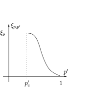
Figure 1: A qualitative plot of $p^{\prime}\mapsto\xi_{p,p^{\prime}}$, for $d=2,3$.

values of $p^{\prime}$ does $\xi_{p,p^{\prime}}\neq\xi_{p}$? Our first main result is the following; see also Figure 1.

Theorem 1.1

Assume that $d\geq 2$, $p<p_{c}$.

The limit in (7) exists for all $0\leq p^{\prime}\leq 1$. Moreover, $p^{\prime}\mapsto\xi_{p,p^{\prime}}$ is Lipschitz continuous and nonincreasing on $[0,1]$, and

$$\xi_{p,p^{\prime}}>0\qquad\forall p^{\prime}\in[0,1).$$

There exists $p^{\prime}_{c}=p^{\prime}_{c}(p,d)\in[p,1)$ such that $\xi_{p,p^{\prime}}=\xi_{p}$ for $p^{\prime}\leq p^{\prime}_{c}$ and $\xi_{p,p^{\prime}}<\xi_{p}$ for $p^{\prime}>p^{\prime}_{c}$. On $(p_{c}^{\prime},1)$, $p^{\prime}\mapsto\xi_{p,p^{\prime}}$ is real analytic and strictly decreasing.

When $d=2,3$, $p^{\prime}_{c}=p$. Moreover, there exist constants $c_{2}^{\pm},c_{3}^{\pm}>0$ such that, as $p^{\prime}\downarrow p_{c}^{\prime}=p$,

$$c_{2}^{-}(p^{\prime}-p)^{2} \leq \xi_{p}-\xi_{p,p^{\prime}}\leq c_{2}^{+}(p^{\prime}-p)^{2}\qquad(d=2),$$ (8)

$$e^{-c_{3}^{-}/(p^{\prime}-p)} \leq \xi_{p}-\xi_{p,p^{\prime}}\leq e^{-c_{3}^{+}/(p^{\prime}-p)}\qquad(d=3).$$ (9)

When $d\geq 4$, $p<p_{c}^{\prime}<1$.

Remark 1.2.

Note that for $d=3$, (9) rules out the possibility of continuing $p^{\prime}\mapsto\xi_{p,p^{\prime}}$ analytically across $p$, to the interval $(0,p)$. It is an open question whether such analytic continuation is possible in two dimensions.

Remark 1.3.

We make a comment regarding the convexity/concavity of $p^{\prime}\mapsto\xi_{p,p^{\prime}}$ for dimensions $2$ and $3$. First, observe that $\xi_{p}$ diverges logarithmically as $p\downarrow 0$, and $\xi_{p,p^{\prime}}\leq\xi_{0,p^{\prime}}=|{\log p^{\prime}}|$. Therefore, since in dimensions $2$ and $3$ the slope of $\xi_{p,p^{\prime}}$ (as a function of $p^{\prime}$) at $p_{c}^{\prime}$ is equal to zero, there must be an inflection point somewhere on the interval $(p_{c}^{\prime},1)$, at least when $p$ is so small that $\xi_{p}>1$. Note also that the above implies that the Lipschitz constant must diverge at least as fast as $|{\log p}|$, as $p\downarrow 0$ (and at most as fast as $1/p$, as the proof shows).

In contrast to the polynomial correction in (5) for the homogeneous case, the presence of defects on the line $\mathcal{L}$ leads to a purely exponential decay of the connectivities, which is the content of our second result:

Theorem 1.4

For all $d\geq 2$ and for all $p^{\prime}>p_{c}^{\prime}$, there exists $\psi_{d}=\psi_{d}(p,p^{\prime})>0$ such that

$$\mathbb{P}_{p,p^{\prime}}(0\leftrightarrow n\mathbf{e}_{1})=\psi_{d}e^{-\xi_{p,p^{\prime}}n}\bigl{(}1+o(1)\bigr{)}.$$ (10)

As will be seen in Section 6, the absence of a polynomial correction in (10) is due to the fact that when $p^{\prime}>p_{c}^{\prime}$, conditionally on $\{0\leftrightarrow n\mathbf{e}_{1}\}$, the cluster containing $0$ and $n\mathbf{e}_{1}$, $C_{0,n\mathbf{e}_{1}}$, is pinned on the line $\mathcal{L}$. Namely, as will be seen in Theorem 6.1, $C_{0,n\mathbf{e}_{1}}$ splits into a string of irreducible components centered on $\mathcal{L}$ and whose sizes have exponential tails.

The analysis of the effects of a line or a (hyper)plane of defects on the qualitative statistical properties of polymers or interfaces has been the subject of a large number of works dating back, at least, to the late 1970s. However, almost all rigorous studies to date have treated the framework of effective models, in which the polymer/interface is modeled by the trajectory of a random walk (or as a random function from $\mathbb{Z}^{d}\to\mathbb{R}$ in the case of higher-dimensional interfaces), and the understanding of such models is by now very detailed Giacomin , Velenik-PS . For example, in the case of a random walk pinned at the origin, one studies the exponential divergence of the partition function

$$Z_{N}^{\varepsilon}=E_{\mathit{RW}}[e^{\varepsilon L_{N}}|X_{N}=0],$$ (11)

where $L_{N}$ is the local time of the random walk $X_{k}$ at the origin up to time $N$, and $\varepsilon>0$ is the pinning parameter (see Appendix B).

There is actually one very particular instance in which it has been possible to investigate these phenomena in a noneffective setting: the 2d Ising model. Indeed, in this case it is sometimes possible to compute explicitly the relevant quantities; see Abraham and references therein. Needless to say, such computations do not convey much understanding of the underlying physics (the desire to get a better understanding of these exact results actually triggered the analysis of effective models!).

On the other hand, new techniques developed during the last decade have lead to a detailed description of structurally one-dimensional objects in various lattice random fields, such as interfaces in 2d Ising and Potts models CIV-Ising , CIV-Potts , GI , large subcritical clusters in (FK-)percolation CIV-Potts , stretched self-interacting polymers IV-annealed , etc.

The effect of a defect line in various systems has recently been the focus of interest in different areas. In particular, Beffara et al. BSSS have started to investigate the influence of defects in the framework of last passage percolation.

It is worthwhile to point out an issue that makes the problem studied in the present paper substantially more subtle than its effective counterpart (11). Namely, a natural way to compare $\xi_{p,p^{\prime}}$ with $\xi_{p}$ is to extract an effective weight for the cluster $C_{0,n\mathbf{e}_{1}}$ connecting $0$ and $n\mathbf{e}_{1}$. That is,

$$\frac{\mathbb{P}_{p,p^{\prime}}(0\leftrightarrow n\mathbf{e}_{1})}{\mathbb{P}_{p}(0\leftrightarrow n\mathbf{e}_{1})} = \sum_{C\ni\{0,n\mathbf{e}_{1}\}}\frac{\mathbb{P}_{p,p^{\prime}}(C_{0,n\mathbf{e}_{1}}=C)}{\mathbb{P}_{p}(0\leftrightarrow n\mathbf{e}_{1})}$$

$$= \sum_{C\ni\{0,n\mathbf{e}_{1}\}}e^{I(C)}\frac{\mathbb{P}_{p}(C_{0,n\mathbf{e}_{1}}=C)}{\mathbb{P}_{p}(0\leftrightarrow n\mathbf{e}_{1})}$$

$$= \mathbb{E}_{p}\bigl{[}e^{I(C_{0,n\mathbf{e}_{1}})}|0\leftrightarrow n\mathbf{e}_{1}\bigr{]},$$

where

$$I(C):=|C\cap\mathcal{L}|\log\frac{p^{\prime}}{p}+|\partial C\cap\mathcal{L}|\log\frac{1-p^{\prime}}{1-p},$$

and $\partial C$ denotes the exterior boundary of the cluster $C$, that is, the set of all edges of $\mathsf{E}^{d}\setminus C$ sharing at least one endpoint with some edge of $C$. Now, observe that in spite of the close resemblance of (1) with (11), there is one major difference: since $\log\frac{p^{\prime}}{p}$ and $\log\frac{1-p^{\prime}}{1-p}$ always have opposite signs, the effective interaction between the cluster and the line $\mathcal{L}$ has both attractive and repulsive components. This is a manifestation of the presence of the “phases” that are neglected in effective models, in which only the polymer/interface is considered and not its environment.

Our analysis of $\mathbb{P}_{p,p^{\prime}}(0\leftrightarrow n\mathbf{e}_{1})$ is based on the use of a geometrical representation of the cluster $C_{0,n\mathbf{e}_{1}}$ as an effective directed random walk. To use this representation effectively for the lower bounds of part 1.1 of Theorem 1.1, the repulsive interaction of the cluster with $\mathcal{L}$ will be handled with a suitable use of the Russo formula.

Random walk representations of subcritical clusters have been used in CampaninoChayesChayes , CampaninoIoffe and CIV-Potts . The one used here is taken from CIV-Potts , and will be described in Section 3. Standard renewal arguments are also recurrent in the paper; a reminder of the main ideas can be found in Appendix A.

1.1 Open problems

Although the picture provided by the present work is quite extensive, we list here some open problems that we think would be particularly interesting to investigate.

1. [(P3)]

2. Properties of $\xi_{p,p^{\prime}}$:

   1. [(a)]

   2. Analyze the behavior of $\xi_{p,p^{\prime}}$ as $p^{\prime}\downarrow p^{\prime}_{c}$, in dimensions $d\geq 4$. In particular, determine whether $\liminf_{p^{\prime}\downarrow p_{c}^{\prime}}\frac{\mathrm{d}\xi_{p,p^{\prime}}}{\mathrm{d}p^{\prime}}<0$ (which we expect to be true in $d\geq 6$, in analogy with the effective case Giacomin ).

   3. Analyze the behavior of $\xi_{p,p^{\prime}}$ as a function of both $p$ and $p^{\prime}$. In particular, for $(p,p^{\prime})$ close to the critical line $p\mapsto p_{c}^{\prime}(p)$.

   4. Determine, for all $p^{\prime}\leq p^{\prime}_{c}$, the sharp asymptotics of the connectivity function $\mathbb{P}_{p,p^{\prime}}(0\leftrightarrow n\mathbf{e}_{1})$, and the corresponding scaling limit of the cluster $C_{0,n\mathbf{e}_{1}}$.

3. Introduce disorder, in which the occupation probabilities of the edges $e\in\mathcal{L}$ are i.i.d. random variables. Study the relevance of disorder. For analogous considerations in the effective/directed case, we refer to AlexZyg , Giacomin , GLT and references therein.

4. More general defects:

   1. [(a)]

   2. Allow a defect line not coinciding with a coordinate axis, which should be amenable to a rather straightforward adaptation of our techniques. Or, as in NewmanWu , consider higher-dimensional defects like hyperplanes of given codimension.

   3. Consider half-space percolation, with the defect line (or hyperplane) at the boundary of the system. Although less natural from the percolation point of view, such a setting is relevant for the analysis of wetting phenomena.

5. In each of the cases mentioned above, study the connectivity $\mathbb{P}_{p,p^{\prime}}(x\leftrightarrow y)$ for generic points $x,y\in\mathbb{Z}^{d}$.

6. Extension to other models. In particular, a version for FK-percolation seems feasible and would provide an extension of our results to Ising/Potts models, which would be very interesting.

We assume throughout the paper that edges outside $\mathcal{L}$ are open with probability $p$, where $p<p_{c}$ is fixed. Furthermore, $c_{i}$, $i=2,3,\ldots,$ will denote constants that can depend on the dimension $d$, on $p$ or $p^{\prime}$, but which remains uniformly bounded away from $0$ and $\infty$ for $(p,p^{\prime})$ belonging to compact subsets of $(0,p_{c})\times(0,1)$.

The line $\mathcal{L}$ will often be identified with $\mathbb{Z}$. We will therefore use the usual terminology related to the total order on $\mathbb{Z}$ (such as “being to the left of” or “being the largest among a set of points”). We will also consider $\mathcal{L}$, without mention, sometimes as a set of edges, and sometimes as a set of sites.

2 Basic properties of $\xi_{p,p^{\prime}}$

In this section, we prove items 1.1 and 1.1 of Theorem 1.1, except for the strict monotonicity and analyticity of $\xi_{p,p^{\prime}}$, which will be proved, respectively, in Sections 6.2 and 6.3.

$\vartriangleright$ Existence of the limit. The existence of the limit in (7) follows from the subadditivity of the sequence $n\mapsto-{\log\mathbb{P}_{p,p^{\prime}}}(0\leftrightarrow n\mathbf{e}_{1})$.

$\vartriangleright$ Monotonicity in $p^{\prime}$ of $\xi_{p,p^{\prime}}$. This follows from a standard coupling argument: if $p_{1}^{\prime}\leq p_{2}^{\prime}$, then $\mathbb{P}_{p,p_{1}^{\prime}}\preccurlyeq\mathbb{P}_{p,p_{2}^{\prime}}$.

$\vartriangleright$ $\xi_{p,p^{\prime}}=\xi_{p}$ for all $p^{\prime}\leq p$. Since $\xi_{p,p^{\prime}}\geq\xi_{p}$ when $p^{\prime}\leq p$, we only need to verify that the reverse inequality also holds. Let $0^{\prime}:=[n^{\alpha}]{\mathbf{e}_{2}}$ and $x^{\prime}:=n\mathbf{e}_{1}+[n^{\alpha}]{\mathbf{e}_{2}}$, where $1/2<\alpha<1$. We can realize $\{0\leftrightarrow n\mathbf{e}_{1}\}$ by connecting $0$ to $0^{\prime}$ and $n\mathbf{e}_{1}$ to $x^{\prime}$ by straight segments of open edges, and by then connecting $0^{\prime}$ to $x^{\prime}$ by an open path: $\mathbb{P}_{p,p^{\prime}}(0\leftrightarrow n\mathbf{e}_{1})\geq(p^{n^{\alpha}})^{2}\mathbb{P}_{p,p^{\prime}}(0^{\prime}\leftrightarrow x^{\prime})$. If we characterize the event $\{0^{\prime}\leftrightarrow x^{\prime}\}$ by the existence of a self-avoiding path $\pi\dvtx 0^{\prime}\to x^{\prime}$,

$$\mathbb{P}_{p,p^{\prime}}(0^{\prime}\leftrightarrow x^{\prime}) \geq \mathbb{P}_{p,p^{\prime}}(\exists\pi\dvtx 0^{\prime}\to x^{\prime},\pi\cap\mathcal{L}=\varnothing)$$

$$= \mathbb{P}_{p}(\exists\pi\dvtx 0^{\prime}\to x^{\prime},\pi\cap\mathcal{L}=\varnothing).$$

But by the van den Berg–Kesten (BK) inequality, (5) and the sharp triangle inequality (3),

$$\mathbb{P}_{p}(\exists\pi\dvtx 0^{\prime}\leftrightarrow x^{\prime},\pi\cap\mathcal{L}\neq\varnothing) \leq \sum_{u\in\mathcal{L}}\mathbb{P}_{p}(0\leftrightarrow u)\mathbb{P}_{p}(u\leftrightarrow x^{\prime})$$

$$\leq \sum_{u\in\mathcal{L}}e^{-\xi_{p}(u-0^{\prime})-\xi_{p}(x^{\prime}-u)}$$

$$\leq e^{-\xi_{p}(x^{\prime}-0^{\prime})}\sum_{u\in\mathcal{L}}e^{-c_{1}(\|u-0^{\prime}\|+\|x^{\prime}-u\|-\|x^{\prime}-0^{\prime}\|)}$$

$$= e^{-O(n^{2\alpha-1})}\mathbb{P}_{p}(0\leftrightarrow n\mathbf{e}_{1}).$$

Therefore, $\mathbb{P}_{p,p^{\prime}}(0\leftrightarrow n\mathbf{e}_{1})\geq p^{2n^{\alpha}}(1-e^{-O(n^{2\alpha-1})})\mathbb{P}_{p}(0\leftrightarrow n\mathbf{e}_{1})$, which implies $\xi_{p,p^{\prime}}\leq\xi_{p}$.

$\vartriangleright$ $\xi_{p,p^{\prime}}<\xi_{p}$ for all $p^{\prime}$ close enough to $1$. Namely, if $p^{\prime}>e^{-\xi_{p}}$, then by opening all the edges of $\mathcal{L}$ between $0$ and $n\mathbf{e}_{1}$,

$$\mathbb{P}_{p,p^{\prime}}(0\leftrightarrow n\mathbf{e}_{1})\geq{p^{\prime}}^{n}=e^{(\log p^{\prime}+\xi_{p})n}e^{-\xi_{p}n}\geq e^{(\log p^{\prime}+\xi_{p})n}\mathbb{P}_{p}(0\leftrightarrow n\mathbf{e}_{1}).$$

The critical value

$$p_{c}^{\prime}=p_{c}^{\prime}(p,d):=\sup\{p^{\prime}\in[0,1]\dvtx\xi_{p,p^{\prime}}=\xi_{p}\}$$

thus separates the regime $\xi_{p,p^{\prime}}=\xi_{p}$ from the one in which $\xi_{p,p^{\prime}}<\xi_{p}$.

$\vartriangleright$ $\xi_{p,p^{\prime}}>0$ for all $0\leq p^{\prime}<1$. Define the slab

$$\mathcal{S}_{u,v}:=\{z\in\mathbb{R}^{d}\dvtx\langle u,\mathbf{e}_{1}\rangle\leq\langle z,\mathbf{e}_{1}\rangle<\langle v,\mathbf{e}_{1}\rangle\}.$$

We divide $\mathcal{L}_{n}:=\mathcal{L}\cap\mathcal{S}_{0,n\mathbf{e}_{1}}$ into blocks of equal lengths $R\in\mathbb{N}$: $B_{j}:=\mathcal{L}_{n}\cap\mathcal{S}_{jR\mathbf{e}_{1},(j+1)R\mathbf{e}_{1}}$, with $j=0,\ldots,[n/R]$. Let also $\mathcal{H}^{-}_{j}=\{x\dvtx\langle x,\mathbf{e}_{1}\rangle<jR\}$, $\mathcal{H}^{+}_{j}=\{x\dvtx\langle x,\mathbf{e}_{1}\rangle\geq(j+1)R\}$. We say that $B_{j}$ is clear if there exists no path of open edges in $\mathcal{L}^{c}$ connecting $\mathcal{L}\cap\mathcal{H}_{j}^{-}$ to $\mathcal{L}\cap\mathcal{H}_{j}^{+}$. We have

$$\qquad\mathbb{P}_{p,p^{\prime}}(0\leftrightarrow n\mathbf{e}_{1})\leq\mathbb{P}_{p,p^{\prime}}(\mbox{each clear block has at least one open edge}).$$ (13)

We show that when $R$ is large, a positive fraction of blocks is clear with high probability. For a cluster $C$ contained in $\mathcal{L}^{c}$, let us define $l(C)$ and $r(C)$ as, respectively, the left-most and right-most points of intersections of the vertex set of $C$ with $\mathcal{L}$. We say that such $C$ is an $(R,n)$-bridge if $r-l\geq R$ and the intersection $[l,r]\cap\mathcal{L}_{n}\neq\varnothing$. Let $C_{1},C_{2},\ldots,C_{M}$ be an enumeration of the disjoint $(R,n)$-bridges. We set $l_{i}=l(C_{i})$ and $r_{i}=r(C_{i})$. By construction, there are disjoint connections from $l_{i}$ to $r_{i}$ in $\mathcal{L}^{c};i=1,\ldots,M$. If $0<\rho<1$, then, using the BK inequality in the last step,

$$\sum_{m=1}^{\infty}\mathbb{P}_{p,p^{\prime}}\Biggl{(}M=m;\sum_{i=1}^{m}\bigl{(}r(C_{i})-l(C_{i})\bigr{)}\geq\rho n\Biggr{)}$$

$$\qquad\leq\sum_{m=1}^{\infty}\mathop{\mathop{\sum_{l_{1},r_{1},\ldots,l_{m},r_{m}}}_{r_{i}-l_{i}>R,}}_{\sum_{i=1}^{m}(r_{i}-l_{i})\geq\rho n}\mathbb{P}_{p,p^{\prime}}\bigl{(}\circ_{1}^{m}\bigl{\{}l_{i}\stackrel{{\scriptstyle\mathcal{L}^{c}}}{{\leftrightarrow}}r_{i}\bigr{\}}\bigr{)}$$

$$\qquad\leq\sum_{m=1}^{\infty}\mathop{\mathop{\sum_{l_{1},r_{1},\ldots,l_{m},r_{m}}}_{r_{i}-l_{i}>R,}}_{\sum_{i=1}^{m}(r_{i}-l_{i})\geq\rho n}\prod_{i=1}^{m}\mathbb{P}_{p,p^{\prime}}\bigl{(}l_{i}\stackrel{{\scriptstyle\mathcal{L}^{c}}}{{\leftrightarrow}}r_{i}\bigr{)},$$

where it is understood that the points $l_{i}$ (resp., $r_{i}$) contributing to the sum are distinct, should in addition satisfy $[l_{i},r_{i}]\cap\mathcal{L}_{n}\neq\varnothing$, and $x\stackrel{{\scriptstyle A}}{{\leftrightarrow}}y$ means that $x$ and $y$ are connected by an open path contained in $A$. Now, $\mathbb{P}_{p,p^{\prime}}(l_{i}\stackrel{{\scriptstyle\mathcal{L}^{c}}}{{\leftrightarrow}}r_{i})=\mathbb{P}_{p}(l_{i}\stackrel{{\scriptstyle\mathcal{L}^{c}}}{{\leftrightarrow}}r_{i})\leq e^{-\xi_{p}|l_{i}-r_{i}|}$. The contribution coming from segments so large that $[l_{i},r_{i}]\supset\mathcal{L}_{n}$ is clearly negligible, and we can restrict our attention to the case when at least one of the endpoints belongs to $\mathcal{L}_{n}$. Since, for all $t>0$, $\mathbf{1}_{\{{X\geq a}\}}\leq e^{t(X-a)}$, this last sum is bounded by

$$e^{-t\rho n}\sum_{m=1}^{n}\mathop{\sum_{l_{1},r_{1},\ldots,l_{m},r_{m}}}_{|l_{i}-r_{i}|>R}\prod_{i=1}^{m}e^{-(\xi_{p}-t)|l_{i}-r_{i}|} \leq c_{2}e^{-t\rho n}\sum_{m=1}^{n}\sum_{l_{1},\ldots,l_{m}}2^{m}e^{-(\xi_{p}-t)mR}$$

$$\leq c_{2}e^{-t\rho n}\bigl{(}1+2e^{-(\xi_{p}-t)R}\bigr{)}^{n}$$

for all $t<\xi_{p}$. By taking $t=\xi_{p}/2$ and $R=\alpha/\xi_{p}$ with $\alpha$ large enough, we get

$$\mathbb{P}_{p,p^{\prime}}\Biggl{(}\sum_{i=1}^{M}|l_{i}-r_{i}|\geq\rho n\Biggr{)}\leq c_{2}e^{-\xi_{p}\rho n/4}.$$

This implies that

$$\mathbb{P}_{p,p^{\prime}}\bigl{(}\mbox{at least $[(1-\rho)n/2R]$ blocks are clear}\bigr{)}\geq 1-c_{2}e^{-\xi_{p}\rho n/4}.$$

Then, conditioned on the event that at least $[(1-\rho)n/2R]$ blocks are clear, the probability on the right-hand side of (13) is bounded above by$\sum_{k\geq[(1-\rho)n/2R]}(1-(1-p^{\prime})^{R})^{k}\leq e^{-c_{3}n}$. Altogether, this shows that $\xi_{p,p^{\prime}}>0$.

$\vartriangleright$ Lipschitz continuity of $\xi_{p,p^{\prime}}$. The proof will rely on the following identity, which follows by Russo’s formula, and which will be used also later in Section 5 (see Grimmett , page 44, for the proof of a similar claim):

Lemma 2.1

For any increasing event $A$ with support in a finite subset of $\mathsf{E}^{d}$, and all $p_{1}^{\prime},p_{2}^{\prime}>0$,

$$\frac{\mathbb{P}_{p,p_{2}^{\prime}}(A)}{\mathbb{P}_{p,p_{1}^{\prime}}(A)}=\exp\int_{p_{1}^{\prime}}^{p_{2}^{\prime}}\frac{1}{s}\mathbb{E}_{p,s}[\#\mathrm{Piv}_{\mathcal{L}}(A)|A]\,\mathrm{d}s,$$ (14)

where $\mathrm{Piv}_{\mathcal{L}}(A)$ is the set of pivotal edges $e\in\mathcal{L}$ for the event $A$.

Let $\mathbb{P}_{p,p^{\prime}}^{(n)}$ denote the restriction of $\mathbb{P}_{p,p^{\prime}}$ to the edges $\mathsf{E}_{n}^{d}$ which lie in the box $\Lambda_{n}:=[-a_{n},a_{n}]^{d}\cap\mathbb{Z}^{d}$. Since $\xi_{p,p^{\prime}}>0$ for all $p^{\prime}<1$, we can assume that $a_{n}\gg n$ is chosen sufficiently large so that for all $n$,

$$\frac{1}{2}\frac{\mathbb{P}_{p,p_{2}^{\prime}}^{(n)}(0\leftrightarrow n\mathbf{e}_{1})}{\mathbb{P}_{p,p_{1}^{\prime}}^{(n)}(0\leftrightarrow n\mathbf{e}_{1})}\leq\frac{\mathbb{P}_{p,p_{2}^{\prime}}(0\leftrightarrow n\mathbf{e}_{1})}{\mathbb{P}_{p,p_{1}^{\prime}}(0\leftrightarrow n\mathbf{e}_{1})}\leq 2\frac{\mathbb{P}_{p,p_{2}^{\prime}}^{(n)}(0\leftrightarrow n\mathbf{e}_{1})}{\mathbb{P}_{p,p_{1}^{\prime}}^{(n)}(0\leftrightarrow n\mathbf{e}_{1})},$$ (15)

when $n$ is large enough. By Lemma 2.1, for any $p_{2}^{\prime}\geq p_{1}^{\prime}\geq p_{c}^{\prime}/2$,

$$\frac{\mathbb{P}_{p,p_{2}^{\prime}}^{(n)}(0\leftrightarrow n\mathbf{e}_{1})}{\mathbb{P}_{p,p_{1}^{\prime}}^{(n)}(0\leftrightarrow n\mathbf{e}_{1})}=\exp\int_{p_{1}^{\prime}}^{p_{2}^{\prime}}\frac{1}{s}\mathbb{E}_{p,s}^{(n)}[\#\mathrm{Piv}_{\mathcal{L}}(0\leftrightarrow n\mathbf{e}_{1})|0\leftrightarrow n\mathbf{e}_{1}]\,\mathrm{d}s.$$ (16)

Given a cluster $C_{0,n\mathbf{e}_{1}}$, let $x$ (resp., $y$) be the leftmost (resp., rightmost) site of $\mathcal{L}\cap C_{0,n\mathbf{e}_{1}}$, and $L:=|x|+|y-n\mathbf{e}_{1}|$. We have

$$\mathbb{E}_{p,s}^{(n)}[\#\mathrm{Piv}_{\mathcal{L}}(0\leftrightarrow n\mathbf{e}_{1})|0\leftrightarrow n\mathbf{e}_{1}]$$

$$\qquad\leq 2n+e^{\xi_{p,s}(1+o(1))n}\sum_{\ell\geq n}(n+\ell)\mathbb{P}_{p,s}^{(n)}(0\leftrightarrow n\mathbf{e}_{1},L=\ell).$$

Since $\mathbb{P}_{p,s}^{(n)}(0\leftrightarrow n\mathbf{e}_{1},L=\ell)\leq\ell\mathbb{P}_{p,s}^{(n)}(0\leftrightarrow(n+\ell)\mathbf{e}_{1})\leq\ell e^{-\xi_{p,s}(n+\ell)}$, we get, using $p_{c}^{\prime}\geq p$,

$$\frac{\mathbb{P}_{p,p_{2}^{\prime}}^{(n)}(0\leftrightarrow n\mathbf{e}_{1})}{\mathbb{P}_{p,p_{1}^{\prime}}^{(n)}(0\leftrightarrow n\mathbf{e}_{1})}\leq\exp\bigl{(}6(p_{2}^{\prime}-p_{1}^{\prime})n/p\bigr{)},$$ (17)

and thus $0\leq\xi_{p,p_{1}^{\prime}}-\xi_{p,p_{2}^{\prime}}\leq 6(p_{2}^{\prime}-p_{1}^{\prime})/p$.

3 Random walk representation of $C_{0,n\mathbf{e}_{1}}$

In this section we recall the description of $C_{0,n\mathbf{e}_{1}}$ in terms of a directed random walk, following CIV-Potts . Since we only consider the direction $\mathbf{e}_{1}$, the representation simplifies in some respects. For instance, the inner products $\langle y,t\rangle$ in CIV-Potts are replaced by $\langle y,\xi_{p}\mathbf{e}_{1}\rangle=\xi_{p}\langle y,\mathbf{e}_{1}\rangle$. The proofs of the main estimates under $\mathbb{P}_{p}$ can be found in CIV-Potts . The reader familiar with CIV-Potts can check the representation formulas (3), (21) and (26), and proceed to Section 4.

Observe that similar arguments for $\mathbb{P}_{p,p^{\prime}}$ will be developed in Section 6.

Let $0<\alpha<1$ be small enough so that the cone

$$\mathcal{Y}^{>}:=\{y\in\mathbb{Z}^{d}\dvtx\langle y,\xi_{p}\mathbf{e}_{1}\rangle\geq(1-\alpha)\xi_{p}(y)\}$$ (18)

has angular aperture at most $\pi/2$. A point $z\in C_{0,n\mathbf{e}_{1}}\neq\varnothing$ is called cone-point if $0<\langle z,\mathbf{e}_{1}\rangle<n$ and $C_{0,n\mathbf{e}_{1}}\subseteq(z+\mathcal{Y}^{>})\cup(z-\mathcal{Y}^{>})$. We order the cone-points according to their first component: $z_{1},\ldots,z_{m+1}$. By construction, $z_{i+1}\in z_{i}+\mathcal{Y}^{>}$. The subgraphs

$$\gamma_{j}:=C_{0,n\mathbf{e}_{1}}\cap\mathcal{S}_{z_{j},z_{j+1}}$$

are called cone-confined irreducible components of $C_{0,n\mathbf{e}_{1}}$; see Figure 2. Note that $\gamma_{j}\subset D(z_{j},z_{j+1})$, where

$$D(z,z^{\prime}):=(z+\mathcal{Y}^{>})\cap(z^{\prime}-\mathcal{Y}^{>}).$$ (19)

The complement $C_{0,n\mathbf{e}_{1}}\setminus(\gamma_{1}\cup\cdots\cup\gamma_{m})$ can contain, at most, two connected components. If it exists, the component containing $0$ (resp., $n\mathbf{e}_{1}$) is denoted $\gamma^{\mathsf{b}}$ (resp., $\gamma^{\mathsf{f}}$), and called backward (resp., forward) irreducible.

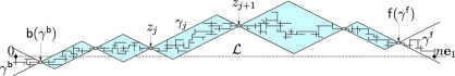
Figure 2: The decomposition of $C_{0,n\mathbf{e}_{1}}$ into irreducible components.

Let ${\mathsf{f}}(\gamma_{j}):=z_{j}$ [resp., ${\mathsf{b}}(\gamma_{j}):=z_{j+1}$] denote the starting (resp., ending) point of $\gamma_{j}$, and ${\mathsf{f}}(\gamma^{\mathsf{f}}):=z_{m}$, ${\mathsf{b}}(\gamma^{\mathsf{b}}):=z_{1}$. Once a set of connected components $\gamma^{\mathrm{b}},\gamma_{1},\ldots,\gamma_{m},\gamma^{\mathsf{f}}$ is given, compatible in the sense that ${\mathsf{f}}(\gamma_{1})={\mathsf{b}}(\gamma^{\mathsf{b}})$, ${\mathsf{b}}(\gamma_{m})={\mathsf{f}}(\gamma^{\mathsf{f}})$, and ${\mathsf{f}}(\gamma_{j})={\mathsf{b}}(\gamma_{j+1})$ if $j=1,\ldots,m-1$, then these can be concatenated ($\sqcup$ denoting the corresponding concatenation operation):

$$\gamma^{\mathrm{b}}\sqcup\gamma_{1}\sqcup\cdots\sqcup\gamma_{m}\sqcup\gamma^{\mathsf{f}}\equiv C_{0,n\mathbf{e}_{1}}.$$

It can be shown that under $\mathbb{P}_{p}$, up to a term of order $e^{-\xi_{p}n-\nu_{1}n}$, the number of cone-confined irreducible components grows linearly with $n$.

Therefore, the probability $\mathbb{P}_{p}(0\leftrightarrow n\mathbf{e}_{1})$ can be decomposed as

$$\mathbb{P}_{p}(0\leftrightarrow n\mathbf{e}_{1})$$

(20)

$$\qquad=\sum_{m\geq 1}\mathop{\sum_{\gamma^{\mathrm{b}},\gamma_{1},\ldots,\gamma_{m},\gamma^{\mathsf{f}}}}_{\mathrm{compat.}}\mathbb{P}_{p}(C_{0,n\mathbf{e}_{1}}=\gamma^{\mathrm{b}}\sqcup\gamma_{1}\sqcup\cdots\sqcup\gamma_{m}\sqcup\gamma^{\mathsf{f}}),$$

where we neglected the configurations with less than two cone-points. One can then define CIV-Potts independent events $\Gamma^{\mathrm{b}}$, $\Gamma_{1},\ldots,\Gamma_{m}$, $\Gamma^{\mathrm{f}}$ such that

$$\quad\mathbb{P}_{p}(C_{0,n\mathbf{e}_{1}}=\gamma^{\mathrm{b}}\sqcup\gamma_{1}\sqcup\cdots\sqcup\gamma_{m}\sqcup\gamma^{\mathsf{f}})=\mathbb{P}_{p}(\Gamma^{\mathrm{b}})\Biggl{(}\prod_{j=1}^{m}\mathbb{P}_{p}(\Gamma_{j})\Biggr{)}\mathbb{P}_{p}(\Gamma^{\mathrm{f}}).$$ (21)

The final step of the construction is to reformulate the rhs of (3) as the probability of an event involving a directed random walk with independent increments. This follows a standard scheme in renewal theory, sketched in Appendix A in a simpler situation, which starts by multiplying (3) by $e^{\xi_{p}n}$.

First, we associate weights to the irreducible components $\gamma^{\mathsf{b}}$ and $\gamma^{\mathsf{f}}$. By translation invariance, we can consider $\gamma^{\mathsf{f}}$ as fixed at the origin, and then translate it at $n\mathbf{e}_{1}$. If $u\in\mathcal{Y}^{>}$ and $v\in-\mathcal{Y}^{>}$, define

$$\qquad\rho_{\mathsf{b}}(u):=e^{\langle u,\xi_{p}\mathbf{e}_{1}\rangle}\mathop{\sum_{\gamma^{\mathrm{b}}\ni 0:}}_{{\mathsf{b}}(\gamma^{\mathsf{b}})=u}\mathbb{P}_{p}(\Gamma^{\mathsf{b}}),\qquad\rho_{\mathsf{f}}(v):=e^{-\langle v,\xi_{p}\mathbf{e}_{1}\rangle}\mathop{\sum_{\gamma^{\mathrm{f}}\ni 0:}}_{{\mathsf{f}}(\gamma^{\mathsf{f}})=v}\mathbb{P}_{p}(\Gamma^{\mathsf{f}}).$$ (22)

These weights satisfy

$$\rho_{\mathsf{b}}(u)\leq e^{-\nu_{2}|u|},\qquad\rho_{\mathsf{f}}(v)\leq e^{-\nu_{2}|v|},$$ (23)

where $\nu_{2}=\nu_{2}(p)>0$.

Remark 3.1.

Since the weights $\rho_{\mathsf{b}}$ and $\rho_{\mathsf{f}}$ have exponentially decaying tails, the sums over $u$ and $v$ [e.g., in the representation formulas (26) and (21) below] can always fix $\alpha>0$ small and restrict attention to the terms for which $|u|,|v|\leq n^{1/2-\alpha}$.

Consider then the cone-confined components $\gamma_{j}$. Define the displacement

$$V(\gamma_{j}):={\mathsf{b}}(\gamma_{j})-{\mathsf{f}}(\gamma_{j}).$$

By translation invariance, all components $\gamma_{j}$ with the same displacement $V(\gamma_{j})=y\in\mathcal{Y}^{>}$ have the same contribution to the sum in (3). We can thus consider only $\gamma_{1}$ and assume that its starting point is the origin: for all $y\in\mathcal{Y}^{>}$,

$${q}(y):=e^{\langle y,\xi_{p}\mathbf{e}_{1}\rangle}\mathop{\sum_{\gamma_{1}:}}_{{\mathsf{f}}(\gamma_{1})=0,{\mathsf{b}}(\gamma_{1})=y}\mathbb{P}_{p}(\Gamma_{1}).$$

By a standard argument (a variant of Appendix A), it can be shown that $q$ defines a probability distribution on $\mathcal{Y}^{>}$. Moreover, there exists $\nu_{3}=\nu_{3}(p)>0$ such that

$$\sum_{y\dvtx|y|\geq t}q(y)\leq e^{-\nu_{3}t}.$$ (24)

Therefore, by summing over $u\in\mathcal{Y}^{>}$ and $v\in-\mathcal{Y}^{>}$, such that $u_{1}<v_{1}$,

$$e^{\xi_{p}n}\mathbb{P}_{p}(0\leftrightarrow n\mathbf{e}_{1})=\\ \sum_{u,v}\rho_{\mathsf{b}}(u)\rho_{\mathsf{f}}(v)\sum_{m\geq 1}\mathop{\sum_{y_{1},\ldots,y_{m}}}_{\sum_{j}y_{j}=n\mathbf{e}_{1}+v-u}\prod_{j=1}^{m}q(y_{j}).$$ (25)

(As before, we neglected the term with less than two cone-points.)

Let us denote by $S=(S_{k})_{k\geq 0}$ the directed random walk on $\mathbb{Z}^{d}$ whose increments $Y_{j}=S_{j}-S_{j-1}\in\mathcal{Y}^{>}$ are i.i.d. and have distribution $q$. When the walk is started at $u$, $S_{0}=u$, we denote its distribution by $\mathrm{P}_{u}$. We can thus write (25) as

$$e^{\xi_{p}n}\mathbb{P}_{p}(0\leftrightarrow n\mathbf{e}_{1})=\sum_{u,v}\rho_{\mathsf{b}}(u)\rho_{\mathsf{f}}(u)\mathrm{P}_{u}\bigl{(}\mathcal{R}(n\mathbf{e}_{1}+v)\bigr{)},$$ (26)

where

$$\mathcal{R}(z):=\{\exists N\geq 1\mbox{ such that }S_{N}=z\}.$$ (27)

More generally, if $A$ is an event measurable with respect to the position of the endpoints of the irreducible components of $C_{0,n\mathbf{e}_{1}}$, that is, to the trajectory of the walk $S$, the same procedure leads to

$$e^{\xi_{p}n}\mathbb{P}_{p}(A\cap\{0\leftrightarrow n\mathbf{e}_{1}\})=\sum_{u,v}\rho_{\mathsf{b}}(u)\rho_{\mathsf{f}}(v)\mathrm{P}_{u}\bigl{(}A\cap\mathcal{R}(n\mathbf{e}_{1}+v)\bigr{)}.$$ (28)

Let $Y_{j}=(Y_{j}^{\parallel},Y_{j}^{\perp})$ be the decomposition of $Y_{j}$ into a longitudinal component $Y_{j}^{\parallel}:=\langle Y_{j},\mathbf{e}_{1}\rangle$ parallel to $\mathbf{e}_{1}$, and a transverse component $Y_{j}^{\perp}\in\mathbb{Z}^{d-1}$ perpendicular to $\mathbf{e}_{1}$. Then:

• $\mathrm{P}_{u}(Y_{1}^{\parallel}\geq 1)=1$;

• $\mathrm{P}_{u}(|Y_{1}|>t)\leq e^{-\nu_{3}t}$ for large $t$;

• for any $z^{\bot}\in\mathbb{Z}^{d-1}$, $\mathrm{P}_{u}(Y_{1}^{\bot}=z_{\bot})=\mathrm{P}_{u}(Y_{1}^{\bot}=-z_{\bot})$.

Since the increments have exponential tails, the following local CLT asymptotics along the direction $n\mathbf{e}_{1}$ hold: fix $\alpha>0$. Then, as $n\to\infty$,

$$\mathrm{P}_{u}\bigl{(}\mathcal{R}(n\mathbf{e}_{1}+v)\bigr{)}=\frac{c_{p}}{n^{({d-1})/{2}}}\bigl{(}1+o(1)\bigr{)}$$ (29)

for some constant $c_{p}>0$, uniformly in $|u|,|v|\leq n^{1/2-\alpha}$. Together with (23) and (26), this in particular leads to the Ornstein–Zernike asymptotics given in (5) (for $x=n\mathbf{e}_{1}$).

4 Upper bounds

We now move on to the proof of the upper bounds of item 1.1, and of item 1.1 of Theorem 1.1. We use (1). Letting $\varepsilon:=\log(p^{\prime}/p)>0$, which is small if $p^{\prime}-p$ is small, we get

$$\frac{\mathbb{P}_{p,p^{\prime}}(0\leftrightarrow n\mathbf{e}_{1})}{\mathbb{P}_{p}(0\leftrightarrow n\mathbf{e}_{1})}\leq\mathbb{E}_{p}\bigl{[}e^{\varepsilon|C_{0,n\mathbf{e}_{1}}\cap\mathcal{L}|}|0\leftrightarrow n\mathbf{e}_{1}\bigr{]}.$$ (30)

We use the random walk representation described in Section 3: $C_{0,n\mathbf{e}_{1}}=\gamma^{\mathsf{b}}\sqcup\gamma_{1}\sqcup\cdots\sqcup\gamma_{m}\sqcup\gamma^{\mathsf{f}}$. If $S$ denotes the effective directed random walk associated to the displacements of the components $\gamma_{i}$, we have

$$|C_{0,n\mathbf{e}_{1}}\cap\mathcal{L}| = |\gamma^{\mathsf{b}}\cap\mathcal{L}|+|\gamma^{\mathsf{f}}\cap\mathcal{L}|+\sum_{i=1}^{m}|\gamma_{i}\cap\mathcal{L}|$$

$$\leq |\gamma^{\mathsf{b}}\cap\mathcal{L}|+|\gamma^{\mathsf{f}}\cap\mathcal{L}|+\sum_{i=1}^{m}|D({S_{i-1},S_{i}})\cap\mathcal{L}|,$$

where the diamond $D(\cdot,\cdot)$ was defined in (19). If $\gamma^{\mathsf{b}}$ ends at $u$, define $\rho_{\mathsf{b}}^{\varepsilon}(u)$ as in (22), with $\mathbb{P}_{p}(\Gamma^{\mathsf{b}})e^{\varepsilon|\gamma^{\mathsf{b}}\cap\mathcal{L}|}$ in place of $\mathbb{P}_{p}(\Gamma^{\mathsf{b}})$. If $\gamma^{\mathsf{f}}$ starts at $v$, $\rho_{\mathsf{f}}^{\varepsilon}(v)$ is defined in the same way. As can be verified, exponential decay as in (23) holds for the weights $\rho_{\mathsf{f}}^{\varepsilon}$ and $\rho_{\mathsf{b}}^{\varepsilon}$, when $\varepsilon$ is sufficiently small. Still following Remark 3.1, we will only consider those $u,v$ with $|u|,|v|\leq n^{1/2-\alpha}$ (for some $0<\alpha<1/2$).

Let $M:=\inf\{j\geq 1\dvtx S_{j}=n\mathbf{e}_{1}+v\}$. Using (28), (29) and (5),

$$\mathbb{E}_{p}\bigl{[}e^{\varepsilon|C_{0,n\mathbf{e}_{1}}\cap\mathcal{L}|}|0\leftrightarrow n\mathbf{e}_{1}\bigr{]}\leq c_{4}\sum_{u,v}\rho_{\mathsf{b}}^{\varepsilon}(u)\rho_{\mathsf{f}}^{\varepsilon}(v)\mathrm{E}_{u,v}\bigl{[}e^{{\varepsilon\sum_{i=1}^{M}}|{D(S_{i-1},S_{i})\cap\mathcal{L}}|}\bigr{]},$$

where $\mathrm{E}_{u,v}[\cdot]=\mathrm{E}_{u}[\cdot|\mathcal{R}(n\mathbf{e}_{1}+v)]$. As we said,

$$\sum_{u,v}\rho_{\mathsf{b}}^{\varepsilon}(u)\rho_{\mathsf{f}}^{\varepsilon}(v)<\infty.$$ (31)

We further decompose

$$\mathrm{E}_{u,v}\bigl{[}e^{{\varepsilon\sum_{i=1}^{M}}|{D(S_{i-1},S_{i})\cap\mathcal{L}}|}\bigr{]}=\sum_{m=1}^{n}\mathrm{E}_{u,v}\bigl{[}e^{{\varepsilon\sum_{i=1}^{m}}|{D(S_{i-1},S_{i})\cap\mathcal{L}}|},{M=m}\bigr{]}.$$

Therefore, for all fixed $1\leq m_{0}\leq n$,

$$\quad\mathrm{E}_{u,v}\bigl{[}e^{{\varepsilon\sum_{i=1}^{M}}|{D(S_{i-1},S_{i})\cap\mathcal{L}}|}\bigr{]}\leq e^{\varepsilon n}\mathrm{P}_{u,v}(M<m_{0})+n\sup_{m_{0}\leq m\leq n}A_{u,v}(m),$$ (32)

where

$$A_{u,v}(m):\! = \mathrm{E}_{u,v}\bigl{[}e^{{\varepsilon\sum_{i=1}^{m}}|{D(S_{i-1},S_{i})\cap\mathcal{L}}|}\bigr{]}$$ (33)

$$= \sum_{k=1}^{m}\mathop{\sum_{\ell_{1},\ldots,\ell_{k}}}_{\sum_{j}\ell_{j}=m}\mathrm{E}_{u,v}\Biggl{[}\prod_{j=1}^{k}\Psi_{\mathcal{L}}(S_{a_{j}-1},S_{a_{j}})\Biggr{]}$$

with $\Psi_{\mathcal{L}}(S_{i-1},S_{i}):=e^{\varepsilon|D(S_{i-1},S_{i})\cap\mathcal{L}|}-1$, and where $\ell_{j}\geq 1$, $a_{j}:=\ell_{1}+\cdots+\ell_{j}$, $a_{0}:=0$.

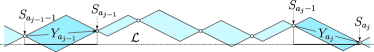
Figure 3: The proof of the upper bound: the size of the intersection of a diamond with $\mathcal{L}$ is bounded above by the size of its projection on $\mathcal{L}$.

Remembering that the cone $\mathcal{Y}^{>}$ has an opening angle of at most $\pi/2$, we have (see Figure 3)

$$|{D(S_{i-1},S_{i})\cap\mathcal{L}}|\leq Y_{i}^{\parallel}\mathbf{1}_{\{{|S_{i-1}^{\bot}|\leq{Y_{i}^{\parallel}}}\}}.$$ (34)

Therefore,

$$\psi_{\mathcal{L}}(S_{i-1},S_{i}) \leq e^{\varepsilon Y_{i}^{\parallel}\mathbf{1}_{\{{|S_{i-1}^{\bot}|\leq{Y_{i}^{\parallel}}}\}}}-1$$

$$= (e^{\varepsilon Y_{i}^{\parallel}}-1)\mathbf{1}_{\{{|{S_{i-1}^{\bot}}|\leq Y_{i}^{\parallel}}\}}$$

$$\leq (e^{\varepsilon}-1)Y_{i}^{\parallel}e^{\varepsilon Y_{i}^{\parallel}}\mathbf{1}_{\{{|{S_{i-1}^{\bot}}|\leq Y_{i}^{\parallel}}\}}$$

$$\equiv (e^{\varepsilon}-1)B(S_{i-1}^{\bot},Y_{i}),$$

which yields

$$A_{u,v}(m) \leq \sum_{k=1}^{m}(e^{\varepsilon}-1)^{k}\mathop{\sum_{\ell_{1},\ldots,\ell_{k}}}_{\sum_{j}\ell_{j}=m}\mathrm{E}_{u,v}\Biggl{[}\prod_{j=1}^{k}B(S_{a_{j}-1}^{\bot},Y_{a_{j}})\Biggr{]}$$

$$\leq O\bigl{(}n^{({d-1})/{2}}\bigr{)}\sum_{k=1}^{m}(e^{\varepsilon}-1)^{k}\mathop{\sum_{\ell_{1},\ldots,\ell_{k}}}_{\sum_{j}\ell_{j}=m}\mathrm{E}_{u}\Biggl{[}\prod_{j=1}^{k}B(S_{a_{j}-1}^{\bot},Y_{a_{j}})\Biggr{]},$$

where (29) was used again. For all $j$, by the Markov property and the local limit theorem in dimension $d-1$ (see Figure 3 and note that the upper bound below is trivial whenever $a_{j-1}=a_{j}-1$),

$$\mathrm{E}_{u}[B(S_{a_{j}-1}^{\bot},Y_{a_{j}})|S_{a_{j-1}},Y_{a_{j}}] = Y_{a_{j}}^{\parallel}e^{\varepsilon Y_{a_{j}}^{\parallel}}\mathrm{P}_{S_{a_{j-1}}}(|{S_{a_{j}-1}^{\bot}}|\leq Y_{a_{j}}^{\parallel})$$

$$\leq Y_{a_{j}}^{\parallel}e^{\varepsilon Y_{a_{j}}^{\parallel}}c_{5}(Y_{a_{j}}^{\parallel})^{d-1}\ell_{j}^{-({d-1})/{2}}.$$

Therefore, since $\mathrm{P}_{u}(Y_{a_{j}}^{\parallel}\geq t)\leq e^{-\nu_{3}t}$,

$$\mathrm{E}_{u}[B(S_{a_{j}-1}^{\bot},Y_{a_{j}})|S_{a_{j-1}}]\leq c_{5}\sum_{t\geq 1}t^{d}e^{\varepsilon t}e^{-\nu_{3}t}\ell_{j}^{-({d-1})/{2}}\equiv c_{6}\ell_{j}^{-({d-1})/{2}}$$

with $c_{6}<\infty$ if $\varepsilon<\nu_{3}$. This gives $A_{u,v}(m)\leq O(n^{({d-1})/{2}})A(m)$, where

$$A(m):=\sum_{k=1}^{m}\bigl{(}c_{6}(e^{\varepsilon}-1)\bigr{)}^{k}\mathop{\sum_{\ell_{1},\ldots,\ell_{k}}}_{\sum_{j}\ell_{j}=m}\prod_{j=1}^{k}\ell_{j}^{-({d-1})/{2}}.$$ (35)

In dimensions $d\geq 4$, we ignore the constraint $\sum_{j}\ell_{j}=m$ and bound $A(m)$ uniformly by

$$A(m)\leq\sum_{k=1}^{\infty}\biggl{\{}c_{6}(e^{\varepsilon}-1)\sum_{\ell\geq 1}\ell^{-({d-1})/{2}}\biggr{\}}^{k},$$

which converges when $\varepsilon>0$ is small enough. Therefore, using (32) with $m_{0}=1$, (30) is

$$\mathbb{E}_{p}\bigl{[}e^{\varepsilon|C_{0,n\mathbf{e}_{1}}\cap\mathcal{L}|}|0\leftrightarrow n\mathbf{e}_{1}\bigr{]}=O\bigl{(}n^{({d+1})/{2}}\bigr{)}.$$

This shows that $\xi_{p,p^{\prime}}\geq\xi_{p}$ when $p^{\prime}-p$ is small enough. Combined with $\xi_{p,p^{\prime}}\leq\xi_{p}$, this implies that $p_{c}^{\prime}(p,d)>p$ in dimensions $d\geq 4$.

In dimensions $d=2$ and $3$, we obtain an upper bound on $A(m)$ which diverges with $m$, in a standard way. As in Appendix A, consider the generating function

$$\mathbb{A}(s):=\sum_{m\geq 1}A(m)s^{m}.$$

Using (35), $\mathbb{A}(s)=\sum_{k\geq 1}\mathbb{B}(s)^{k}$ where $\mathbb{B}(s):=c_{6}(e^{\varepsilon}-1)\sum_{\ell\geq 1}\ell^{-({d-1})/{2}}s^{\ell}$. Let $\phi(\varepsilon)>0$ be the unique number for which

$$\mathbb{B}\bigl{(}e^{-\phi(\varepsilon)}\bigr{)}=1.$$ (36)

We have $\mathbb{A}(e^{-2\phi(\varepsilon)})<\infty$, and therefore $A(m)\leq e^{2\phi(\varepsilon)m}$ for all large enough $m$. Using (32) with $m_{0}=c_{7}n$ with $c_{7}>0$ small enough, and taking $\varepsilon$ small enough, (30) is bounded by

$$\mathbb{E}_{p}\bigl{[}e^{\varepsilon|C_{0,n\mathbf{e}_{1}}\cap\mathcal{L}|}|0\leftrightarrow n\mathbf{e}_{1}\bigr{]}\leq c_{8}\bigl{(}1+O\bigl{(}n^{({d-1})/{2}}\bigr{)}e^{2\phi(\varepsilon)n}\bigr{)}.$$

This shows that $\xi_{p}-\xi_{p,p^{\prime}}\leq 2\phi(\varepsilon)$. Using Giacomin , Theorem A.2, in (36), the asymptotics of $\phi(\varepsilon)$ when $\varepsilon\downarrow 0$ is seen to be

$$\phi(\varepsilon)=\cases{c_{9}\varepsilon^{2}\bigl{(}1+o(1)\bigr{)}&\quad$(d=2)$,\vspace*{2pt}\cr{e^{-c_{10}/\varepsilon(1+o(1))}}&\quad$(d=3)$.}$$

5 Lower bounds

We prove the lower bounds of item 1.1 of Theorem 1.1, in $d=2,3$, for $p^{\prime}>p$, with $p^{\prime}-p$ small enough. We will need the following rough estimate on the connectivity under $\mathbb{P}_{p,p^{\prime}}$:

Lemma 5.1

Set

$$\xi^{*}_{p}:=\min_{\mathbf{n}\in\mathbb{S}^{d-1}}\xi_{p}(\mathbf{n})>0.$$ (37)

For all $p<p_{c}$, there exists $\eta=\eta(p)>0$ such that, for all $p^{\prime}<p+\eta$,

$$\mathbb{P}_{p,p^{\prime}}(x\leftrightarrow y)\leq e^{-c_{11}\xi_{p}^{*}|y-x|},$$

uniformly in $x,y\in\mathbb{Z}^{d}$.

Let $\ell(x,y):=|C_{x,y}\cap\mathcal{L}|$. Proceeding as in (1),

$$\mathbb{P}_{p,p^{\prime}}(x\leftrightarrow y)\leq\mathbb{E}_{p}\bigl{[}e^{\ell(x,y)\log(p^{\prime}/p)};x\leftrightarrow y\bigr{]}.$$

Since $\mathbb{P}_{p}(x\leftrightarrow y;\ell(x,y)=l)\leq e^{-c_{12}\xi_{p}^{*}|x-y|\wedge l}$, the claim follows.

Recall that $\mathbb{P}_{\cdot}^{(n)}$ denotes the restriction of $\mathbb{P}_{\cdot}$ to the edges $\mathsf{E}_{n}^{d}$ which lie inside a large box $\Lambda_{n}$, so that by (15)

$$\frac{\mathbb{P}_{p,p^{\prime}}(0\leftrightarrow n\mathbf{e}_{1})}{\mathbb{P}_{p}(0\leftrightarrow n\mathbf{e}_{1})}\geq\frac{1}{2}\frac{\mathbb{P}_{p,p^{\prime}}^{(n)}(0\leftrightarrow n\mathbf{e}_{1})}{\mathbb{P}_{p}^{(n)}(0\leftrightarrow n\mathbf{e}_{1})}.$$

Let $\mathcal{P}_{n}$ denote the collection of self-avoiding nearest-neighbor paths $\pi\dvtx 0\to n\mathbf{e}_{1}$ contained in $\Lambda_{n}$. Let $\pi=(\pi_{0},\pi_{1},\ldots,\pi_{m})\in\mathcal{P}_{n}$, that is, $\pi_{0}=0$ and $\pi_{m}=n\mathbf{e}_{1}$. We say that $\pi_{i}$ is a cone-point of $\pi$ if $0<\langle\pi_{i},\mathbf{e}_{1}\rangle<n$ and $\pi\subset(\pi_{i}-\mathcal{Y}^{>})\cup(\pi_{i}+\mathcal{Y}^{>})$.

Let $\delta>0$, and define

$$\mathcal{M}_{\delta}:=\{\mbox{$\exists$ an open path $\pi\in\mathcal{P}_{n}$ with at least $\delta n$ cone-points on $\mathcal{L}_{n}$}\}.$$

We emphasize the crucial fact that we do not require that cone-points of open paths are cone-points of the whole cluster $C_{0,n\mathbf{e}_{1}}$. This ensures that $\mathcal{M}_{\delta}$ is an increasing event: once a configuration contains a suitable open path, opening additional edges will never remove this path (observe also that suitability of an open path only depends on its geometry, not on the state of other edges in the configuration).

Since $\{0\leftrightarrow n\mathbf{e}_{1}\}\supset\mathcal{M}_{\delta}$, we can write

$$\frac{\mathbb{P}_{p,p^{\prime}}^{(n)}(0\leftrightarrow n\mathbf{e}_{1})}{\mathbb{P}_{p}^{(n)}(0\leftrightarrow n\mathbf{e}_{1})}\geq\frac{\mathbb{P}_{p,p^{\prime}}^{(n)}(\mathcal{M}_{\delta})}{\mathbb{P}_{p}^{(n)}(0\leftrightarrow n\mathbf{e}_{1})}=\frac{\mathbb{P}_{p,p^{\prime}}^{(n)}(\mathcal{M}_{\delta})}{\mathbb{P}_{p}^{(n)}(\mathcal{M}_{\delta})}\mathbb{P}_{p}^{(n)}(\mathcal{M}_{\delta}|0\leftrightarrow n\mathbf{e}_{1}).$$

The terms in the last display are, respectively, the energy gain and the entropy cost for restricting to the event $\mathcal{M}_{\delta}$. These will be studied separately. First:

Proposition 5.2

Let $d\geq 2$. There exists $c_{13}=c_{13}(p,p^{\prime})>0$ such that, for all $p^{\prime}>p$, $p^{\prime}-p$ small enough, and all $n\in\mathbb{N}$,

$$\frac{\mathbb{P}_{p,p^{\prime}}^{(n)}(\mathcal{M}_{\delta})}{\mathbb{P}_{p}^{(n)}(\mathcal{M}_{\delta})}\geq e^{c_{13}\delta(p^{\prime}-p)n}.$$

Then, we check that $\mathcal{M}_{\delta}$ is not too unlikely under $\mathbb{P}_{p}^{(n)}(\cdot|0\leftrightarrow n\mathbf{e}_{1})$:

Proposition 5.3

There exist $c_{14}=c_{14}(p)>0$ and $c_{15}=c_{15}(p)>0$ such that for small enough $\delta>0$,

$$\mathbb{P}_{p}^{(n)}(\mathcal{M}_{\delta}|0\leftrightarrow n\mathbf{e}_{1})\geq\cases{e^{-c_{14}\delta^{2}n}&\quad$(d=2)$,\cr e^{-c_{15}(\delta/|{\log\delta}|)n}&\quad$(d=3)$.}$$

Putting these bounds together, an appropriate choice of $\delta$ as a function of $p^{\prime}-p$ leads to the lower bounds of item 1.1 of Theorem 1.1. Namely,

$$\delta:=\cases{c_{13}(p^{\prime}-p)/(2c_{14}),&\quad in $d=2$,\vspace*{2pt}\cr e^{-2c_{15}/(c_{13}(p^{\prime}-p))},&\quad in $d=3$.}$$

5.1 Proof of Proposition 5.2

First, observe that

$$\mathrm{Piv}_{\mathcal{L}\cap\Lambda_{n}}(\mathcal{M}_{\delta})\supset\mathrm{Piv}_{\mathcal{L}\cap\Lambda_{n}}(0\leftrightarrow n\mathbf{e}_{1})\qquad\mbox{on the event }\mathcal{M}_{\delta}.$$

Indeed, let $e\in\mathrm{Piv}_{\mathcal{L}\cap\Lambda_{n}}(0\leftrightarrow n\mathbf{e}_{1})$. Then $e$ must belong to all paths $\pi$ satisfying the conditions prescribed in the event $\mathcal{M}_{\delta}$ (since removing this edge disconnects $0$ from $n\mathbf{e}_{1}$). This shows that $e$ is pivotal for $\mathcal{M}_{\delta}$.

We start by using Lemma 2.1: by the preceding observation and the fact that $\mathcal{M}_{\delta}$ is increasing, we obtain

$$\frac{\mathbb{P}^{(n)}_{p,p^{\prime}}(\mathcal{M}_{\delta})}{\mathbb{P}^{(n)}_{p}(\mathcal{M}_{\delta})} = \exp\int_{p}^{p^{\prime}}\frac{1}{s}\mathbb{E}^{(n)}_{p,s}[\#\mathrm{Piv}_{\mathcal{L}\cap\Lambda_{n}}(\mathcal{M}_{\delta})|\mathcal{M}_{\delta}]\,\mathrm{d}s$$

$$\geq \exp\int_{p}^{p^{\prime}}\frac{1}{s}\mathbb{E}^{(n)}_{p,s}[\#\mathrm{Piv}_{\mathcal{L}\cap\Lambda_{n}}(0\leftrightarrow n\mathbf{e}_{1})|\mathcal{M}_{\delta}]\,\mathrm{d}s$$

$$\geq \exp\int_{p}^{p^{\prime}}\frac{1}{s}\mathbb{E}^{(n)}_{p,s}[\#\mathrm{Piv}_{\mathcal{L}_{n}}(0\leftrightarrow n\mathbf{e}_{1})|\mathcal{M}_{\delta}]\,\mathrm{d}s.$$

Our goal is thus to bound $\#\mathrm{Piv}_{\mathcal{L}_{n}}(0\leftrightarrow n\mathbf{e}_{1})$ from below on $\mathcal{M}_{\delta}$.

Let us fix an arbitrary total ordering on $\mathcal{P}_{n}$. For each $\pi\in\mathcal{P}_{n}$, let $\mathcal{E}_{\pi}\subset\mathcal{M}_{\delta}$ denote the event on which $\pi$ is the smallest open path having at least $\delta n$ cone-points on $\mathcal{L}_{n}$. Then

$$\mathbb{E}^{(n)}_{p,s}[\#\mathrm{Piv}_{\mathcal{L}_{n}}(0\leftrightarrow n\mathbf{e}_{1})|\mathcal{M}_{\delta}]$$

(39)

$$\qquad=\sum_{\pi\in\mathcal{P}_{n}}\mathbb{E}^{(n)}_{p,s}[\#\mathrm{Piv}_{\mathcal{L}_{n}}(0\leftrightarrow n\mathbf{e}_{1})|\mathcal{E}_{\pi}]\mathbb{P}^{(n)}_{p,s}(\mathcal{E}_{\pi}|\mathcal{M}_{\delta}).$$

Let $\mathsf{E}^{d}_{n,\pi}:=\mathsf{E}^{d}_{n}\setminus\pi$. We say that a cone-point $\pi_{s}\in\mathcal{L}_{n}$ is covered if

$$(\pi_{s}-\mathcal{Y}^{>})\stackrel{{\scriptstyle\mathsf{E}^{d}_{n,\pi}}}{{\longleftrightarrow}}(\pi_{s}+\mathcal{Y}^{>}),$$

uncovered otherwise.

Lemma 5.4

Given $\pi\in\mathcal{P}_{n}$ and $\rho>0$ define the event

$${\mathrm{A}}_{\pi}(\rho,n)=\{\mbox{A fraction $\geq\rho$ of $\pi$'s cone-points on $\mathcal{L}_{n}$ are uncovered}\}.$$

Let $s-p>0$ be sufficiently small. Then there exists $\rho=\rho(p)>0$ such that for all $\pi\in\mathcal{P}_{n}$ compatible with $\mathcal{M}_{\delta}$,

$$\mathbb{P}_{p,s}^{(n)}\bigl{(}{\mathrm{A}}_{\pi}(\rho,n)|\mathcal{E}_{\pi}\bigr{)}\geq\tfrac 12.$$ (40)

Observe that each uncovered cone-point of $\pi$ on $\mathcal{L}_{n}$ has two incident edges $e\in\mathcal{L}_{n}$ which are pivotal for $\{0\leftrightarrow n\mathbf{e}_{1}\}$. Therefore, by (40),

$$\mathbb{E}^{(n)}_{p,s}[\#\mathrm{Piv}_{\mathcal{L}_{n}}(0\leftrightarrow n\mathbf{e}_{1})|\mathcal{E}_{\pi}]\geq\tfrac{1}{2}\times\rho{\delta n},$$

which, together with (5.1) and (5.1), completes the proof of Proposition 5.2. Proof of Lemma 5.4 Fix some path $\pi$ realizing $\mathcal{M}_{\delta}$. We claim first that, as probability measures on $\{0,1\}^{\mathsf{E}^{d}_{n,\pi}}$,

$$\mathbb{P}_{p,s}^{(n)}(\cdot|\mathcal{E}_{\pi})\preccurlyeq\mathbb{P}_{p,s}^{(n)}(\cdot).$$ (41)

Indeed, note that if $\omega\in\mathcal{E}_{\pi}\subseteq\{0,1\}^{\mathsf{E}^{d}_{n,\pi}}$, then for every edge $e\in\mathsf{E}_{n,\pi}^{d}$, the configuration $\omega_{e}^{0}$ defined by

$$\omega_{e}^{0}(b)=\cases{\omega(b),&\quad if $b\neq e$,\cr 0,&\quad if $b=e$,}$$

belongs to $\mathcal{E}_{\pi}$ as well. In particular, any two configurations $\omega,\omega^{\prime}\in\mathcal{E}_{\pi}$ are connected via a sequence of bond flips within $\mathcal{E}_{\pi}$. Furthermore, for every $\eta\in\mathcal{E}_{\pi}$ and for any edge $e\in\mathsf{E}_{n,\pi}^{d}$,

$$\mathbb{P}_{p,s}^{(n)}\bigl{(}\omega(e)=1|\omega|_{\mathsf{E}_{n,\pi}^{d}\setminus\{e\}}=\eta;\mathcal{E}_{\pi}\bigr{)}$$

$$\qquad=\cases{0,&\quad if $e$ is pivotal for $\mathcal{E}_{\pi}$ in $\eta$,\cr\mathbb{P}_{p,s}^{(n)}\bigl{(}\omega(e)=1\bigr{)},&\quad otherwise.}$$

Thus, (41) follows from a a standard dynamic coupling argument for two Markov chains on $\{0,1\}^{\mathsf{E}_{n,\pi}^{d}}$, which are reversible with respect to $\mathbb{P}_{p,s}^{(n)}(\cdot)$ and $\mathbb{P}_{p,s}^{(n)}(\cdot|\mathcal{E}_{\pi})$ accordingly.

The event ${\mathrm{A}}_{\pi}(\rho,n)$ is $\mathsf{E}_{n,\pi}^{d}$-measurable and decreasing. Hence, in order to prove (40) it would be enough to show that $\mathbb{P}_{p,s}^{(n)}({\mathrm{A}}_{\pi}(\rho,n))\geq\frac{1}{2}$ for all $\mathcal{M}_{\delta}$-compatible paths $\pi\in\mathcal{P}_{n}$.

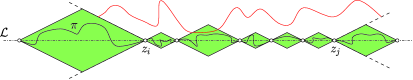
Figure 4: The event $\{z_{i}\leftrightsquigarrow z_{j}\}$.

Let us fix such a $\pi$, and denote the cone-points of $\pi$ on $\mathcal{L}_{n}$, ordered from left to right, by $z_{1},\ldots,z_{M}$, $M\geq\delta n$. We denote by $z_{i}\leftrightsquigarrow z_{j}$ ($i<j$) the event (see Figure 4)

$$(z_{i}-\mathcal{Y}^{>})\stackrel{{\scriptstyle\mathsf{E}_{n,\pi}^{d}}}{{\longleftrightarrow}}(z_{j}+\mathcal{Y}^{>}).$$

By construction the events $z_{i}\leftrightsquigarrow z_{j}$ are $\mathsf{E}_{n,\pi}^{d}$-measurable and increasing.

Observe that if $\pi$ has $m$ of its points $z_{j}$ covered, then there must exist a set of distinct pairs $\{z_{k_{j}},z_{k_{j}^{\prime}}\}\subset\{z_{1},\ldots,z_{M}\}$, $j=1,\ldots,q$, such that: [(2)]

$\sum_{j=1}^{q}|k_{j}^{\prime}-k_{j}+1|=m$;

$\{z_{k_{1}}\leftrightsquigarrow z_{k_{1}^{\prime}}\}\circ\cdots\circ\{z_{k_{q}}\leftrightsquigarrow z_{k_{q}^{\prime}}\}$. By the BK inequality,

$$\mathbb{P}_{p,s}^{(n)}(\{z_{k_{1}}\leftrightsquigarrow z_{k_{1}^{\prime}}\}\circ\cdots\circ\{z_{k_{q}}\leftrightsquigarrow z_{k_{q}^{\prime}}\})\leq\prod_{j=1}^{q}\mathbb{P}_{p,s}^{(n)}(z_{k_{j}}\leftrightsquigarrow z_{k_{j}^{\prime}}).$$

Now, it follows from Lemma 5.1 that if $s-p$ is small enough, and $|z_{k_{j}}-z_{k_{j}^{\prime}}|\geq c_{16}/\xi_{p}^{*}$,

$$\mathbb{P}_{p,s}^{(n)}(z_{k_{j}}\leftrightsquigarrow z_{k_{j}^{\prime}}) \leq \mathop{\sum_{x\in z_{k_{j}}-\mathcal{Y}^{>}}}_{y\in z_{k_{j}^{\prime}}+\mathcal{Y}^{>}}e^{-(c_{11}\xi_{p}^{*}/2)(|x-y|+1)}\leq c_{17}e^{-(c_{11}\xi_{p}^{*}/2)|z_{k_{j}}-z_{k_{j}^{\prime}}|}$$

$$\leq e^{-c_{18}(|{k_{j}^{\prime}}-{k_{j}}|+1)}.$$

On the other hand, if $|z_{k_{j}}-z_{k_{j}^{\prime}}|\leq c_{16}/\xi_{p}^{*}$, then

$$\mathbb{P}_{p,s}^{(n)}(z_{k_{j}}\leftrightsquigarrow z_{k_{j}^{\prime}})\leq\mathbb{P}_{p,s}^{(n)}(z_{k_{j}}\mbox{ is covered})\leq e^{-c_{19}}\leq e^{-c_{20}(|{k_{j}^{\prime}}-{k_{j}}|+1)}.$$

Indeed, if $B_{R}(z)$ is the Euclidean ball of radius $R$ centered at $z$, and $\mathcal{B}:=\{\mbox{all edges of $B_{R}(z_{k_{j}})$ are closed}\}$ with $R=c_{21}/\xi_{p}^{*}$ with $c_{21}>0$ large enough, then

$$\mathbb{P}_{p,s}^{(n)}(z_{k_{j}}\mbox{ is not covered})\geq\mathbb{P}_{p,s}^{(n)}(z_{k_{j}}\mbox{ is covered}\,|\mathcal{B})\mathbb{P}_{p,s}^{(n)}(\mathcal{B})\geq\tfrac{1}{2}\times e^{-c_{22}R^{d}}.$$

Therefore, it follows from (41) and the above discussion that with $c_{23}:=c_{18}\wedge c_{20}$,

$$\mathbb{P}_{p,s}^{(n)}(\mbox{a fraction $\geq\alpha$ of $\pi$'s cone-points on $\mathcal{L}_{n}$ are covered}\,|\mathcal{E}_{\pi})$$

$$\qquad\leq\sum_{m=\alpha M}^{M}\pmatrix{M\cr m}e^{-c_{23}m}\leq e^{-c_{24}M}\leq e^{-c_{24}\delta n}$$

once $\alpha$ is close enough to $1$. This proves the lemma.

5.2 Proof of Proposition 5.3

We use the representation of $C_{0,n\mathbf{e}_{1}}$ in terms of the directed random walk $S$. Observe that if $S$ hits $\mathcal{L}_{n}$, a cone-point is created. Therefore, let $\mathcal{C}_{\delta}$ denote the event in which the trajectory of $S$ hits $\mathcal{L}_{n}$ at least $\delta n$ times after time $n=0$. Using (28) and keeping only configurations with empty boundary clusters, $\gamma^{\mathsf{b}}=\gamma^{\mathsf{f}}=\varnothing$,

$$e^{\xi_{p}n}\mathbb{P}_{p}(\mathcal{M}_{\delta})\geq\mathrm{P}_{0}(\mathcal{C}_{\delta}\cap\mathcal{R}_{n}),$$

where $\mathcal{R}_{n}:=\mathcal{R}(n\mathbf{e}_{1})$. Dividing by $e^{\xi_{p}n}\mathbb{P}_{p}^{(n)}(0\leftrightarrow n\mathbf{e}_{1})\leq e^{\xi_{p}n}\mathbb{P}_{p}(0\leftrightarrow n\mathbf{e}_{1})$ and using (5) and (29), we get

$$\mathbb{P}_{p}^{(n)}(\mathcal{M}_{\delta}|0\leftrightarrow n\mathbf{e}_{1})\geq c_{25}\mathrm{P}_{0}(\mathcal{C}_{\delta}|\mathcal{R}_{n}),$$ (42)

where $c_{25}>0$ does not depend on $n$. The next step is to express $\mathrm{P}_{0}(\mathcal{C}_{\delta}|\mathcal{R}_{n})$ in terms of $S^{\parallel}$ and $S^{\bot}$. Let $\tau_{0}:=0$, and for $k\geq 1$, $\tau_{k}:=\inf\{m>\tau_{k-1}:S_{m}\in\mathcal{L}\}$. Using (29) we infer that for all $n$ and $k\leq n/2$, $\mathrm{P}_{0}(\mathcal{R}_{n-k})/\mathrm{P}_{0}(\mathcal{R}_{n})\geq c_{26}$ for some $c_{26}>0$, and so by the strong Markov property,

$$\mathrm{P}_{0}(\mathcal{C}_{\delta}|\mathcal{R}_{n}) = \mathrm{P}_{0}\bigl{(}S^{\|}_{\tau_{\lfloor\delta n\rfloor}}\leq n|\mathcal{R}_{n}\bigr{)}$$

$$= \sum_{k\leq n/2}\mathrm{P}_{0}\bigl{(}S^{\|}_{\tau_{\lfloor\delta n\rfloor}}=k\bigr{)}\mathrm{P}_{0}(\mathcal{R}_{n-k})/\mathrm{P}_{0}(\mathcal{R}_{n})$$

$$\geq c_{26}\mathrm{P}_{0}\bigl{(}S^{\|}_{\tau_{\lfloor\delta n\rfloor}}\leq n/2\bigr{)}.$$

Let $\bar{n}:=n\mathrm{E}[Y_{1}^{\parallel}]/4$. If $\mathcal{N}^{\parallel}_{n}:=\max\{k\leq n\dvtx S_{k}^{\parallel}\leq n/2\}$ denotes the number of steps performed by $S$ before leaving the strip $\mathcal{S}_{0,n\mathbf{e}_{1}/2}$,

$$\mathrm{P}_{0}\bigl{(}S^{\|}_{\tau_{\lfloor\delta n\rfloor}}\leq n/2\bigr{)} \geq \mathrm{P}_{0}\bigl{(}S^{\|}_{\tau_{\lfloor\delta n\rfloor}}\leq n/2;\mathcal{N}^{\parallel}_{n}\geq\bar{n}\bigr{)}$$

$$\geq \mathrm{P}_{0}\bigl{(}L^{\perp}(\bar{n})\geq\delta n,\mathcal{N}^{\parallel}_{n}\geq\bar{n}\bigr{)}$$

with $L^{\perp}(\bar{n})=\#\{0\leq i\leq\bar{n}\dvtx S^{\perp}_{i}=0\}$. By an elementary large deviation estimate, $\mathrm{P}_{0}(\mathcal{N}^{\parallel}_{n}<\bar{n})\leq e^{-c_{27}n}$ for some $c_{27}>0$. Therefore,

$$\mathrm{P}_{0}\bigl{(}L^{\perp}(\bar{n})\geq\delta n,\mathcal{N}^{\parallel}_{n}\geq\bar{n}\bigr{)} \geq \mathrm{P}_{0}\bigl{(}L^{\perp}(\bar{n})\geq\delta n\bigr{)}-e^{-c_{27}n}$$

$$= \mathrm{P}_{0}\bigl{(}L^{\perp}(\bar{n})\geq\delta_{*}\bar{n}\bigr{)}-e^{-c_{27}n},$$

where $\delta_{*}=4\delta/\mathrm{E}[Y_{1}^{\parallel}]$. The event $\{L^{\perp}(\bar{n})\geq\delta_{*}\bar{n}\}$ depends only on the transverse component $S^{\perp}$, which lies in $\mathbb{Z}^{d-1}$. It follows from Corollary B.3 in Appendix B that

$$\mathrm{P}_{0}\bigl{(}L^{\perp}(\bar{n})\geq\delta_{*}\bar{n}\bigr{)}\geq\cases{e^{-c\delta_{*}^{2}n}&\quad$(d=2)$,\vspace*{2pt}\cr e^{-c(\delta_{*}/|{\log\delta_{*}}|)n}&\quad$(d=3)$.}$$

This proves Proposition 5.3.

6 Proof of Theorem 1.4

In this section we prove Theorem 1.4: when $p^{\prime}>p_{c}^{\prime}$, $\mathbb{P}_{p,p^{\prime}}(0\leftrightarrow n\mathbf{e}_{1})$ has a purely exponential decay. The underlying mechanism is that when $\xi_{p}>\xi_{p,p^{\prime}}$, a typical cluster $C_{0,n\mathbf{e}_{1}}$ connecting $0$ to $n\mathbf{e}_{1}$ is pinned on $\mathcal{L}_{n}$, in the sense that it has a number of cone-points on $\mathcal{L}_{n}$ that grows linearly with $n$. Cone-points of $C_{0,n\mathbf{e}_{1}}$ lying on $\mathcal{L}_{n}$ will be called cone-renewals.

Theorem 6.1

If $p^{\prime}>p_{c}^{\prime}$, then there exist $\delta=\delta(p,p^{\prime})>0$ and $\nu_{4}=\nu_{4}(p,p^{\prime})>0$ such that for any large enough $n$,

$$\mathbb{P}_{p,p^{\prime}}(C_{0,n\mathbf{e}_{1}}\mbox{ has less than $\delta n$ cone-renewals}\,|0\leftrightarrow n\mathbf{e}_{1})\leq e^{-\nu_{4}n}.$$ (43)

With this piece of information, irreducible components with both endpoints on $\mathcal{L}$ can be defined, and a fairly standard renewal argument leads to the pure exponential decay. (Note, however, that at this point we do not even know whether under $\mathbb{P}_{p,p^{\prime}}$ the cluster $C_{0,n\mathbf{e}_{1}}$ contains cone-points at all.)

The presence of cone-points on $\mathcal{L}$ will also allow to complete the proof of Theorem 1.1: we show in Section 6.2 that $p^{\prime}\mapsto\xi_{p,p^{\prime}}$ is strictly decreasing on $(p_{c}^{\prime},1)$, and in Section 6.2 that it is real analytic on the same interval.

Assume $p^{\prime}>p_{c}^{\prime}$, and let

$$\tau:=\xi_{p}-\xi_{p,p^{\prime}}>0.$$

To prove Theorem 6.1, we will first show that $C_{0,n\mathbf{e}_{1}}$ typically stays in a vicinity of size $|{\log\tau}|/\tau$ of $\mathcal{L}_{n}$. This implies, by a finite-energy argument, that $C_{0,n\mathbf{e}_{1}}$ is made of many stretches on which cone-renewals occur with positive probability.

6.1 Excursions away from $\mathcal{L}$

To any realization of $\{0\leftrightarrow n\mathbf{e}_{1}\}$, we associate the smallest self-avoiding path $\pi\dvtx 0\to n\mathbf{e}_{1}$ contained in $C_{0,n\mathbf{e}_{1}}$, as in Section 5.1: $\pi=(\pi_{0},\pi_{1},\ldots,\pi_{|\pi|})$, with $\pi_{0}=0$, $\pi_{|\pi|}=n\mathbf{e}_{1}$.

Let $K\geq 1$, which will be chosen later as a function of $\tau$. Let also

$$\tau_{K}(s):=\inf\{t>s\dvtx\pi_{t}\notin B_{K}(\pi_{s})\}.$$

We associate to $\pi$ a set of disjoint pairs $(u_{1},v_{1}),\ldots,(u_{m},v_{m})$ of points lying on $\mathcal{L}$, as follows; see Figure 5. Let $t_{0}:=0$, and set, for $j\geq 1$,

$$s_{j} := \inf\{s\geq t_{j-1}\dvtx\pi(s)\in\mathcal{L},\pi[s+1,\tau_{K}(s)]\cap\mathcal{L}=\varnothing\},$$

$$t_{j} := \inf\{t>s_{j}\dvtx\pi_{t}\in\mathcal{L}\}.$$

We call the subpath $\mathcal{X}_{j}:=\pi[s_{j},t_{j}]$ an excursion, starting at $u_{j}:=\pi_{s_{j}}$ and ending at $v_{j}:=\pi_{t_{j}}$.

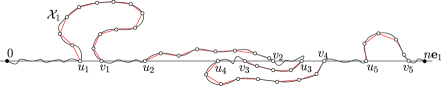
Figure 5: Coarse-graining the excursions of a path $\pi\dvtx 0\to n\mathbf{e}_{1}$.

We further coarse-grain each excursion $\mathcal{X}_{j}$ on the scale $K$. Let $u_{j}^{0}:=u_{j}$ and, for $k\geq 0$,

$$u_{j}^{k+1}:=\pi_{\tau_{K}(u_{j}^{k})}.$$

If $m_{j}:=\max\{k\dvtx u_{j}^{k}\in\mathcal{X}_{j}\}$, we call $\#_{K}\mathcal{X}_{j}:=m_{j}$ the length of the excursion $\mathcal{X}_{j}$ (measured by the number of increments of size $K$). The set of points $(u_{j}^{0}\equiv u_{j},u_{j}^{1},\ldots,u_{j}^{m_{j}},v_{j})$ is called the skeleton of $\mathcal{X}_{j}$. Sometimes, $u_{j}^{{m_{j}}}\equiv v_{j}$, but in all cases, $|u_{j}^{m_{j}}-v_{j}|\leq K$.

We denote by $\{u\stackrel{{\scriptstyle m}}{{\curvearrowright}}v\}$ the event in which there exists a path which is an excursion of length $m$ starting at $u$ and ending at $v$.

Lemma 6.2

There exists $K_{0}=K_{0}(\tau)$ and $c_{28}=c_{28}(\tau)>0$ such that if $K\geq K_{0}$,

$$\mathbb{P}_{p,p^{\prime}}\bigl{(}u\stackrel{{\scriptstyle m}}{{\curvearrowright}}v\bigr{)}\leq e^{-\xi_{p,p^{\prime}}|v-u|-c_{28}\tau Km}.$$

Denote by $\mathcal{X}$ any excursion occurring in $\{u\stackrel{{\scriptstyle m}}{{\curvearrowright}}v\}$. That is, $\#_{K}\mathcal{X}=m$. Let $(u^{0},\ldots,u^{m})$ be a skeleton, where for the sake of simplicity, we assume that $u^{m}=v$. By construction, the event

$$\{\mathcal{X}\mbox{ has skeleton $(u^{0},\ldots,u^{m})$}\}$$

implies that there are disjoint connections $u^{0}\stackrel{{\scriptstyle\mathcal{L}^{c}}}{{\leftrightarrow}}u^{1},\ldots,u^{m-1}\stackrel{{\scriptstyle\mathcal{L}^{c}}}{{\leftrightarrow}}u^{m}$. By the BK inequality,

$$\mathbb{P}_{p,p^{\prime}}\bigl{(}\mathcal{X}\mbox{ has skeleton $(u^{0},\ldots,u^{m})$}\bigr{)} \leq \prod_{i=1}^{m}\mathbb{P}_{p,p^{\prime}}\bigl{(}u^{i-1}\stackrel{{\scriptstyle\mathcal{L}^{c}}}{{\leftrightarrow}}u^{i}\bigr{)}$$

$$\leq \prod_{i=1}^{m}\mathbb{P}_{p}(u^{i-1}\leftrightarrow u^{i})$$

$$\leq \prod_{i=1}^{m}e^{-\xi_{p}(u^{i}-u^{i-1})}.$$

If $z\in\mathbb{R}^{d}$, let $k\in\{1,\ldots,d\}$ be such that $\langle\mathbf{e}_{k},z\rangle={\max_{k^{\prime}}}|\langle\mathbf{e}_{k^{\prime}},z\rangle|$. Then, using (2) and since $\xi_{p}\mathbf{e}_{k}\in\partial W_{p}$,

$$\xi_{p}(z) = \sup_{t\in\partial W_{p}}\langle t,z\rangle\geq\xi_{p}\langle\mathbf{e}_{k},z\rangle=\xi_{p,p^{\prime}}\langle\mathbf{e}_{k},z\rangle+\tau\langle\mathbf{e}_{k},z\rangle$$

$$\geq \xi_{p,p^{\prime}}|\langle\mathbf{e}_{1},z\rangle|+c_{29}\tau|z|$$

for some constant $c_{29}=c_{29}(d)>0$. Since

$$\sum_{i=1}^{m}|\langle\mathbf{e}_{1},u^{i}-u^{i-1}\rangle|\geq|v-u|$$

and $|u^{i}-u^{i-1}|\geq K$ for all $i=1,\ldots,m$, we get

$$\mathbb{P}_{p,p^{\prime}}\bigl{(}\mathcal{X}\mbox{ has skeleton $(u^{i})_{i=0,\ldots,m}$}\bigr{)}\leq e^{-\xi_{p,p^{\prime}}|v-u|-c_{29}\tau Km}.$$

When $u^{m}\neq v$, a similar computation leads to the same bound. Since the number of skeletons with $m$ increments is $O((K^{d-1})^{m}K^{d})$, the conclusion follows by taking $K\geq K_{0}$, with $K_{0}$ large enough in order that $\frac{\log K_{0}}{K_{0}}$ be sufficiently small compared to $\tau$.

Let $\#_{K}\pi:=\sum_{j}\#_{K}\mathcal{X}_{j}$ denote the total number of increments in the excursions of $\pi$.

Proposition 6.3

Let $0<\varepsilon<1$. There exists $K_{1}=K_{1}(\tau,\varepsilon)$ and $c_{30}=c_{30}(\varepsilon)>0$ such that for all $K\geq K_{1}$,

$$\mathbb{P}_{p,p^{\prime}}(\#_{K}\pi\geq\varepsilon n/K|0\leftrightarrow n\mathbf{e}_{1})\leq e^{-c_{30}n}.$$ (44)

For a collection of triples $(u_{j},v_{j},m_{j})_{j=1}^{M}$, let $\mathcal{P}((u_{j},v_{j},m_{j})_{j=1}^{M})$ denote the event on which there exists a path $\pi\dvtx 0\to n\mathbf{e}_{1}$ with $M$ excursions, the $j$th excursion $\mathcal{X}_{j}$, starting at $u_{j}$ and ending at $v_{j}$, and being such that $\#_{K}\mathcal{X}_{j}=m_{j}$. The event $\mathcal{P}((u_{j},v_{j},m_{j})_{j=1}^{M})$ implies the disjoint occurrence

$$\{v_{0}\leftrightarrow u_{1}\}\circ\bigl{\{}u_{1}\stackrel{{\scriptstyle m_{1}}}{{\curvearrowright}}v_{1}\bigr{\}}\circ\cdots\circ\{v_{M-1}\leftrightarrow u_{M}\}\circ\bigl{\{}u_{M}\stackrel{{\scriptstyle m_{M}}}{{\curvearrowright}}v_{M}\bigr{\}}.$$

Assuming $K$ is larger than the $K_{0}$ of Lemma 6.2, and by the BK inequality,

$$\mathbb{P}_{p,p^{\prime}}(\mathcal{P}((u_{j},v_{j},m_{j})_{j=1}^{M})) \leq \prod_{j=1}^{M}\mathbb{P}_{p,p^{\prime}}(v_{j-1}\leftrightarrow u_{j})\mathbb{P}_{p,p^{\prime}}\bigl{(}u_{j}\stackrel{{\scriptstyle m_{j}}}{{\curvearrowright}}v_{j}\bigr{)}$$

$$\leq \prod_{j=1}^{M}e^{-\xi_{p,p^{\prime}}(|u_{j}-v_{j-1}|+|v_{j}-u_{j}|)}e^{-c_{28}\tau Km_{j}}.$$

We then sum over the triples $(u_{j},v_{j},m_{j})_{j=1}^{M}$. Denote by $I\supset\mathcal{L}_{n}$ the smallest interval of $\mathcal{L}$ containing all the points $u_{j},v_{j}$, $j=1,\ldots,M$. Observe that $\sum_{j=1}^{M}(|u_{j}-v_{j-1}|+|v_{j}-u_{j}|)\geq|I|$. We first sum over the possible positions of $I$, then over the positions of the $M\geq 1$ distinct points $u_{j}$ in $I$, then over the $m_{j}$’s satisfying $\sum_{j=1}^{M}m_{j}\geq\varepsilon n/K$, and finally over the endpoints $v_{j}$. Since to a given point $u_{j}$ correspond at most $2K(m_{j}+1)$ points $v_{j}$,

$$\mathbb{P}_{p,p^{\prime}}(\#_{K}\pi\geq\varepsilon n/K,0\leftrightarrow n\mathbf{e}_{1})$$

$$\qquad\leq\sum_{I\supset\mathcal{L}_{n}}e^{-\xi_{p,p^{\prime}}|I|}\sum_{M\geq 1}\pmatrix{|I|\cr M}\mathop{\sum_{m_{1},\ldots,m_{M}\geq 1}}_{\sum_{j}m_{j}\geq\varepsilon n/K}\prod_{j=1}^{M}\bigl{(}2K(m_{j}+1)\bigr{)}e^{-c_{28}\tau Km_{j}}.$$

We choose $K_{1}\geq K_{0}$ large enough so that, for all $K\geq K_{1}$ and all $m\geq 1$, $(2K(m+1))e^{-c_{28}\tau Km}\leq e^{-c_{31}\tau Km}$. Proceeding as on page 2,

$$\sum_{M\geq 1}\pmatrix{|I|\cr M}\mathop{\sum_{m_{1},\ldots,m_{M}\geq 1}}_{\sum_{j}m_{j}\geq\varepsilon n/K}\prod_{j=1}^{M}e^{-c_{31}\tau Km_{j}}\leq e^{c_{32}e^{-c_{31}\tau K/2}|I|}.$$ (45)

Then, notice that there are $\ell-n$ intervals $I\supset\mathcal{L}_{n}$ of fixed length $|I|=\ell$. Therefore, summing over $|I|$ gives

$$\mathbb{P}_{p,p^{\prime}}(\#_{K}\pi\geq\varepsilon n/K,0\leftrightarrow n\mathbf{e}_{1})\leq e^{-c_{33}\tau\varepsilon n}e^{-\xi_{p,p^{\prime}}n}.$$

Since $\mathbb{P}_{p,p^{\prime}}(0\leftrightarrow n\mathbf{e}_{1})=e^{-\xi_{p,p^{\prime}}(1+o(1))n}$ as $n\to\infty$, we get (44) once $K$ is sufficiently large.

We then turn to the study of the deviations of $C_{0,n\mathbf{e}_{1}}$ away from its smallest connecting path $\pi\subset C_{0,n\mathbf{e}_{1}}$.

Let $\pi$ be a given path, which we here consider together with its set of edges. Let $R_{0}:=\max\{|z-0|\dvtx 0\stackrel{{\scriptstyle\pi^{c}}}{{\leftrightarrow}}z\}$ and $z_{0}\in C_{0,n\mathbf{e}_{1}}$ be any point at which the max is attained. Let $\hat{\pi}^{0}$ be the smallest path realizing the connection between $0$ and $z_{0}$, disjoint from $\pi$. Inductively, for $s=1,\ldots,|\pi|$, let $\Pi_{s}:=\bigcup_{0\leq t<s}\hat{\pi}^{t}$,

$$R_{s}:=\max\bigl{\{}|z-\pi_{s}|\dvtx\pi_{s}\stackrel{{\scriptstyle{(\pi\cup\Pi_{s})^{c}}}}{{\longleftrightarrow}}z\bigr{\}},$$

$z_{s}\in C_{0,n\mathbf{e}_{1}}$ be any point at which the max is attained, and $\hat{\pi}^{s}$ be any path realizing the connection between $\pi_{s}$ and $z_{s}$, disjoint from $\pi\cup\Pi_{s}$.

Proposition 6.4

Let $0<\varepsilon<1$. There exists $K_{3}=K_{3}(p,p^{\prime},\varepsilon)$ and $c_{34}=c_{34}(p,p^{\prime},\varepsilon)>0$ such that if $K\geq K_{3}$, then

$$\mathbb{P}_{p,p^{\prime}}\Biggl{(}\sum_{s=0}^{|\pi|}R_{s}\mathbf{1}_{\{{R_{s}\geq K}\}}\geq\varepsilon n\Big{|}0\leftrightarrow n\mathbf{e}_{1}\Biggr{)}\leq e^{-c_{34}n}.$$ (46)

We know from Proposition 6.3 that under $\mathbb{P}_{p,p^{\prime}}(\cdot|0\leftrightarrow n\mathbf{e}_{1})$, the number of increments of the skeleton of a typical path $\pi\dvtx 0\to n\mathbf{e}_{1}$ is at most $\varepsilon n/K$. We can therefore assume, in particular, that

$$|\pi|\leq c_{35}K^{d-1}n.$$ (47)

For a fixed path $\pi$, let $\mathcal{F}_{\pi}$ denote the event in which $\pi$ is the smallest self-avoiding path connecting $0$ to $n\mathbf{e}_{1}$. Arguing as for (41), we get $\mathbb{P}_{p,p^{\prime}}(\cdot|\mathcal{F}_{\pi})\preccurlyeq\mathbb{P}_{p,p^{\prime}}(\cdot)$ on $\pi^{c}$. The event $\{\sum_{s=0}^{|\pi|}R_{s}\mathbf{1}_{\{{R_{s}\geq K}\}}\geq\varepsilon n\}$ is $\pi^{c}$-measurable and increasing. Therefore, by the BK inequality and Lemma 5.1,

$$\mathbb{P}_{p,p^{\prime}}\Biggl{(}\sum_{s=0}^{|\pi|}R_{s}\mathbf{1}_{\{{R_{s}\geq K}\}}\geq\varepsilon n\Big{|}\mathcal{F}_{\pi}\Biggr{)}$$

$$\qquad\leq\mathbb{P}_{p,p^{\prime}}\Biggl{(}\sum_{s=0}^{|\pi|}R_{s}\mathbf{1}_{\{{R_{s}\geq K}\}}\geq\varepsilon n\Biggr{)}$$

$$\qquad\leq\mathop{\mathop{\sum_{r_{1},\ldots,r_{|\pi|}:}}_{\sum_{s}r_{s}\geq\varepsilon n,}}_{r_{s}\geq K}\mathop{\sum_{z_{1},\ldots,z_{|\pi|}:}}_{|z_{s}-\pi_{s}|=r_{s}}\mathbb{P}_{p,p^{\prime}}\bigl{(}\{\pi_{0}\leftrightarrow z_{0}\}\circ\cdots\circ\bigl{\{}\pi_{|\pi|}\leftrightarrow z_{|\pi|}\bigr{\}}\bigr{)}$$

$$\qquad\leq\mathop{\mathop{\sum_{r_{1},\ldots,r_{|\pi|}:}}_{\sum_{s}r_{s}\geq\varepsilon n,}}_{r_{s}\geq K}\prod_{s=0}^{|\pi|}c_{36}r_{s}^{d-1}e^{-c_{11}\xi_{p}^{*}r_{s}}.$$

The proof then follows the same lines as before: if $K$ is large enough, then $c_{36}r^{d-1}e^{-c_{11}\xi_{p}^{*}r}\leq e^{-c_{37}r}$ for all $r\geq K$. The summation can thus be done as in (45), and using (47) gives (46).

Let $\mathcal{T}_{2K}$ be the tube containing points whose Euclidean distance to $\mathcal{L}$ is $\leq 2K$, and consider the cone

$$\mathcal{Y}:=\{x\dvtx\langle x,\mathbf{e}_{1}\rangle\geq|x^{\perp}|\}.$$

For each $x\in\mathcal{L}^{c}$, let $z_{+}$ (resp., $z_{-}$) denote the largest (resp., smallest) point of $\mathcal{L}$ such that $x\in z_{+}-\mathcal{Y}$ (resp., $x\in z_{-}+\mathcal{Y}$). The segment $[z_{-},z_{+}]$ is called the shade of $x$. Let $\mathcal{S}_{n}\subset\mathcal{L}_{n}$ be the set of points of $\mathcal{L}_{n}$ who lie in the shade of at least one point of $C_{0,n\mathbf{e}_{1}}\cap(\mathcal{T}_{2K})^{c}$. The points of $\mathcal{R}_{n}:=\mathcal{L}_{n}\setminus\mathcal{S}_{n}$ are candidates for being cone-renewals.

It is easy to see that

$$|\mathcal{S}_{n}|\leq c_{38}K\sum_{j}\#_{K}\mathcal{X}_{j}+c_{39}K\sum_{s=0}^{|\pi|}R_{s}\mathbf{1}_{\{{R_{s}\geq K}\}},$$

where $c_{38}$ and $c_{39}$ depend only on the dimension $d$. As a corollary of Propositions 6.3 and 6.4, $|\mathcal{S}_{n}|=O(\varepsilon n)$. More precisely, for a fixed $0<\eta<1$, $K$ can be taken large enough so that

$$\mathbb{P}_{p,p^{\prime}}\bigl{(}|\mathcal{R}_{n}|\geq(1-\eta)n|0\leftrightarrow n\mathbf{e}_{1}\bigr{)}\geq 1-e^{-c_{40}n}$$ (48)

with $c_{40}>0$ depending on $p$, $p^{\prime}$ and $\eta$. Proof of Theorem 6.1 We apply a local surgery under $\mathbb{P}_{p,p^{\prime}}(\cdot|0\leftrightarrow n\mathbf{e}_{1})$, to show that $\mathcal{L}_{n}$ contains many cone-renewals (see Figure 6). Consider the partition of $\mathcal{T}_{n}$ into neighboring disjoint blocks

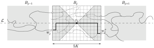
Figure 6: The local surgery inside the block $B_{j}$, turning a pre-renewal $z_{j}$ into a cone-renewal: open a minimal path (in bold) connecting $w_{j}^{-}$ to $w_{j}^{+}$, and close all other edges of $B_{j}$ (dotted). By the finite energy property, this event has probability $p_{*}=e^{-O(K^{d})}>0$.

$B_{j}$ of lengths $5K$, centered at points $z_{j}$. If $z_{j}\in\mathcal{R}_{n}$, we call $z_{j}$ a pre-renewal. Assume $z_{j}$ is a pre-renewal. Let $F_{j}^{-}$, $F_{j}^{+}$ denote the two faces of $B_{j}$ which are orthogonal to $\mathcal{L}_{n}$, and let $W_{j}^{-}\subset F_{j}^{-}$ (resp., $W_{j}^{+}\subset F_{j}^{+}$) denote the points of $C_{0,n\mathbf{e}_{1}}\cap F_{j}^{-}$ (resp., $C_{0,n\mathbf{e}_{1}}\cap F_{j}^{+}$) which are connected to $0$ (resp., $n\mathbf{e}_{1}$) by a path not intersecting $B_{j}$. Let $w_{j}^{\pm}$ denote the smallest point (in lexicographical order) of $F_{j}^{\pm}$. Under $\mathbb{P}_{p,p^{\prime}}(\cdot|w_{j}^{-},w_{j}^{+},0\leftrightarrow n\mathbf{e}_{1})$, independently of the edges living outside $B_{j}$, $w_{j}^{-}$ is connected to $w_{j}^{+}$ by a minimal path going through $z_{j}$, turning $z_{j}$ into a cone-renewal with positive probability, bounded below by some $p_{*}>0$ depending on $K$.

The variables $X_{i}:=\mathbf{1}_{\{{z_{i}\ \mathrm{is}\ \mathrm{a}\ \mathrm{cone}\mbox{-}\mathrm{renewal}}\}}$ can thus be coupled to i.i.d. Bernoulli variables $Y_{i}$ of parameter $p$, giving

$$\mathbb{P}_{p,p^{\prime}}\Biggl{(}\sum_{i=1}^{n/5K}X_{i}\leq p_{*}n/(10K)\Big{|}0\leftrightarrow n\mathbf{e}_{1}\Biggr{)}\leq\mathrm{P}\Biggl{(}\sum_{i=1}^{n/5K}Y_{i}\leq p_{*}n\Big{/}(10K)\Biggr{)}\leq e^{-c_{41}n}.$$

Together with (48), this proves the claim.

Let us complete the proof of Theorem 1.4. We first define the irreducible components $\zeta_{j}$ of $C_{0,n\mathbf{e}_{1}}$, which are cone-confined and which, in contrast to the $\gamma_{j}$ of Section 3, have both their endpoints on $\mathcal{L}_{n}$.

Let us denote by $\{w_{1},\ldots,w_{m+1}\}\subset C_{0,n\mathbf{e}_{1}}$ the cone-renewals that lie on $\mathcal{L}_{n}$, ordered according to their first component. By Theorem 6.1, $m$ is typically of order $n$. The subgraphs

$$\zeta_{j}:=C_{0,n\mathbf{e}_{1}}\cap\mathcal{S}_{w_{j},w_{j+1}}$$

are called cone-confined irreducible components of $C_{0,n\mathbf{e}_{1}}$. The complement $C_{0,n\mathbf{e}_{1}}\setminus(\zeta_{1}\cup\cdots\cup\zeta_{m})$ can contain, at most, two connected components. If it exists, the component containing $0$ (resp., $n\mathbf{e}_{1}$) is denoted $\zeta^{\mathsf{b}}$ (resp., $\zeta^{\mathsf{f}}$), and called backward (forward) irreducible. Keeping in mind that we are here working with the cone $\mathcal{Y}$ rather than $\mathcal{Y}^{>}$ and that the edges on $\mathcal{L}$ are opened with probability $p^{\prime}$, all the definitions of Section 3 extend with almost no changes to the irreducible components $\zeta$. In particular, we can define independent events $\Xi^{\mathsf{b}},\Xi_{1},\ldots,\Xi_{m},\Xi^{\mathsf{f}}$ so that

$$\mathbb{P}_{p,p^{\prime}}(C_{0,n\mathbf{e}_{1}}=\zeta^{\mathsf{b}}\sqcup\zeta_{1}\sqcup\cdots\sqcup\zeta_{m}\sqcup\zeta^{\mathsf{f}})=\mathbb{P}_{p,p^{\prime}}(\Xi^{\mathsf{b}})\Biggl{(}\prod_{j=1}^{m}\mathbb{P}_{p,p^{\prime}}(\Xi_{j})\Biggr{)}\mathbb{P}_{p,p^{\prime}}(\Xi^{\mathsf{f}}).$$

One can thus define, for $u\geq 1$, $v\leq-1$,

$$\rho_{\mathsf{b}}^{\prime}(u):=e^{\xi_{p,p^{\prime}}u}\mathop{\sum_{\zeta^{\mathsf{b}}\ni 0:}}_{{\mathsf{b}}(\zeta^{\mathsf{b}})=u}\mathbb{P}_{p,p^{\prime}}(\Xi^{\mathsf{b}}),\qquad\rho_{\mathsf{f}}^{\prime}(v):=e^{\xi_{p,p^{\prime}}|v|}\mathop{\sum_{\zeta^{\mathsf{f}}\ni 0:}}_{{\mathsf{f}}(\zeta^{\mathsf{f}})=v}\mathbb{P}_{p,p^{\prime}}(\Xi^{\mathsf{f}}).$$

By (43), these weights satisfy the following bounds:

$$\rho_{\mathsf{b}}^{\prime}(u)\leq e^{-\nu_{4}|u|},\qquad\rho_{\mathsf{f}}^{\prime}(v)\leq e^{-\nu_{4}|v|}.$$ (49)

Moreover, $q^{\prime}(\ell):=e^{\xi_{p,p^{\prime}}\ell}f_{\ell}$ with

$$f_{\ell}:=\mathop{\sum_{\zeta_{1}\ni 0:}}_{{\mathsf{f}}(\zeta_{1})=0,{\mathsf{b}}(\zeta_{1})=\ell}\mathbb{P}_{p,p^{\prime}}(\Xi_{1})$$ (50)

defines a probability distribution on $\mathbb{N}$. Again, by (43),

$$f_{\ell}\leq e^{-\xi_{p,p^{\prime}}\ell-\nu_{4}\ell},$$ (51)

which implies

$$q^{\prime}(\ell)\leq e^{-\nu_{4}\ell}.$$ (52)

Up to a term of order $e^{-\nu_{4}n}$ [compare with (25)],

$$\quad e^{\xi_{p,p^{\prime}}n}\mathbb{P}_{p,p^{\prime}}(0\leftrightarrow n\mathbf{e}_{1})=\sum_{u,v}\rho_{\mathbf{b}}^{\prime}(u)\rho_{\mathbf{f}}^{\prime}(v)\sum_{m\geq 1}\mathop{\sum_{\ell_{1},\ldots,\ell_{m}:}}_{\sum_{j}\ell_{j}=n+v-u}\prod_{j=1}^{m}q^{\prime}(\ell_{j}).$$ (53)

As before, due to (49), the sum in (53) can be restricted to those $u,v$ that satisfy $|u|,|v|\leq n^{1/2-\alpha}$, for some small $\alpha>0$. Let thus $\tau_{k}$, $k\geq 1$, be an i.i.d. sequence with distribution $Q^{\prime}(\tau_{1}=\ell):=q^{\prime}(\ell)$. Then, (53) writes

$$e^{\xi_{p,p^{\prime}}}\mathbb{P}_{p,p^{\prime}}(0\leftrightarrow n\mathbf{e}_{1})$$

$$\qquad=\sum_{u,v}\rho_{\mathbf{b}}^{\prime}(u)\rho_{\mathbf{f}}^{\prime}(v)Q^{\prime}\Biggl{(}\exists m\geq 1\mbox{ such that }\sum_{j=1}^{m}\tau_{j}=n+v-u\Biggr{)}.$$

By (52), $E_{Q^{\prime}}[\tau_{1}]<\infty$. Moreover, $q^{\prime}(\ell)>0$ for all $\ell\geq 1$, and therefore, by the renewal theorem,

$$Q^{\prime}\Biggl{(}\exists m\geq 1\mbox{ such that }\sum_{j=1}^{m}\tau_{j}=n+v-u\Biggr{)}\to\frac{1}{E_{Q^{\prime}}[\tau_{1}]}$$

as $n\to\infty$, uniformly in $|u|,|v|\leq n^{1/2-\alpha}$. This proves Theorem 1.4.

6.2 Strict monotonicity of $p^{\prime}\mapsto\xi_{p,p^{\prime}}$

Assume $p^{\prime}>p^{\prime}_{c}$, that is, $\xi_{p,p^{\prime}}<\xi_{p}$. Consider the measures $\mathbb{P}_{p,p^{\prime}}^{(n)}$ defined in Section 5. If $a_{n}\gg n$ is taken large enough, then we can write $\xi_{p,p^{\prime}}=\lim_{n\to\infty}\xi_{p,p^{\prime}}^{(n)}$, where

$$\xi_{p,p^{\prime}}^{(n)}:=-\frac{1}{n}\log\mathbb{P}_{p,p^{\prime}}^{(n)}(0\leftrightarrow n\mathbf{e}_{1}).$$

Therefore,

$$\frac{\mathrm{d}\xi_{p,p^{\prime}}^{(n)}}{\mathrm{d}p^{\prime}}=-\frac{1}{n}\frac{\mathrm{d}\mathbb{P}_{p,p^{\prime}}^{(n)}(0\leftrightarrow n\mathbf{e}_{1})/{\mathrm{d}p^{\prime}}}{\mathbb{P}_{p,p^{\prime}}^{(n)}(0\leftrightarrow n\mathbf{e}_{1})}.$$

By Theorem 6.1, the expected number of cone-renewals under $\mathbb{P}_{p,p^{\prime}}(\cdot|0\leftrightarrow n\mathbf{e}_{1})$ grows linearly with $n$. Since each cone-renewal is adjacent to two edges which are pivotal for $\{0\leftrightarrow n\mathbf{e}_{1}\}$, we can use Russo’s Formula as before to find a constant $c_{42}>0$ such that

$$\frac{1}{n}\frac{\mathrm{d}\mathbb{P}_{p,p^{\prime}}^{(n)}(0\leftrightarrow n\mathbf{e}_{1})/{\mathrm{d}p^{\prime}}}{\mathbb{P}_{p,p^{\prime}}^{(n)}(0\leftrightarrow n\mathbf{e}_{1})}\geq c_{42}.$$

This implies that $\frac{\mathrm{d}\xi_{p,p^{\prime}}^{(n)}}{\mathrm{d}p^{\prime}}\leq-c_{42}$, uniformly in $n$. $p^{\prime}\mapsto\xi_{p,p^{\prime}}$ is therefore strictly decreasing on $(p_{c}^{\prime},1)$, since for all $p_{c}^{\prime}<p_{1}^{\prime}<p_{2}^{\prime}<1$,

$$\xi_{p,p_{2}^{\prime}}-\xi_{p,p_{1}^{\prime}}=\lim_{n\to\infty}\bigl{(}\xi_{p,p_{2}^{\prime}}^{(n)}-\xi_{p,p_{1}^{\prime}}^{(n)}\bigr{)}=\lim_{n\to\infty}\int_{p_{1}^{\prime}}^{p_{2}^{\prime}}\frac{\mathrm{d}\xi_{p,p^{\prime}}^{(n)}}{\mathrm{d}p^{\prime}}\,\mathrm{d}p^{\prime}\leq-c_{42}(p_{2}^{\prime}-p_{1}^{\prime}).$$

6.3 Analyticity of $p^{\prime}\mapsto\xi_{p,p^{\prime}}$

Fix $p<p_{c}$. Consider $f_{\ell}=f_{\ell}(p^{\prime})$ defined in (50). Observe that $f_{\ell}$ can be put in the form of a polynomial in $p^{\prime}$, $f_{\ell}(p^{\prime})=\sum_{k=0}^{\ell}a_{k}^{(\ell)}p^{\prime k}$, with $a_{k}^{(\ell)}\geq 0$. It can therefore be continued as an analytic function $w\mapsto f_{\ell}(w)$ in the complex plane. Let

$$\Phi(w,z):=\sum_{\ell\geq 1}f_{\ell}(w)e^{z\ell}.$$

Since

$$\Phi(p^{\prime},\xi_{p,p^{\prime}})=\sum_{\ell\geq 1}f_{\ell}(p^{\prime})e^{\xi_{p,p^{\prime}}\ell}=\sum_{\ell\geq 1}q^{\prime}(\ell)=1,$$

the analyticity of $p^{\prime}\mapsto\xi_{p,p^{\prime}}$ will follow by solving $\Phi(w,z)=1$ for $z$, in a neighborhood of $(p^{\prime},\xi_{p,p^{\prime}})$. To do so, we must verify that $(w,z)\mapsto\Phi(w,z)$ is analytic in a domain of $\mathbb{C}^{2}$ containing $(p^{\prime},\xi_{p,p^{\prime}})$, and that $\frac{\partial\Phi}{\partial z}|_{(p^{\prime},\xi_{p,p^{\prime}})}\neq 0$. If $w\in D_{\delta}(p^{\prime}):=\{w\in\mathbb{C}\dvtx|w-p^{\prime}|<\delta\}$,

$$|f_{\ell}(w)|\leq\sum_{k=0}^{\ell}a_{k}^{(\ell)}|w|^{k}\leq\sum_{k=0}^{\ell}a_{k}^{(\ell)}(p^{\prime}+\delta)^{k}\leq(1+\delta/p^{\prime})^{\ell}f_{\ell}(p^{\prime}).$$

We can therefore choose $\delta=\delta(p,p^{\prime})>0$ small enough to ensure that

$$\sup_{w\in D_{\delta}(p^{\prime})}\biggl{|}\frac{f_{\ell}(w)}{f_{\ell}(p^{\prime})}\biggr{|}\leq e^{\nu_{4}\ell/3}.$$

We also take $\varepsilon>0$ such that $\sup_{z\in D_{\varepsilon}(\xi_{p,p^{\prime}})}|e^{z\ell}|\leq e^{(\xi_{p,p^{\prime}}+\nu_{4}/3)\ell}$. Remembering the bound for $f_{\ell}(p^{\prime})$ in (51), we thus get

$$\sum_{\ell\geq 1}\sup_{w\in D_{\delta}(p^{\prime})}\sup_{z\in D_{\varepsilon}(\xi_{p,p^{\prime}})}|f_{\ell}(w)e^{z\ell}|<\infty.$$

Therefore, $\Phi$ defines an analytic function of $(w,z)$ in the polydisc $D_{\delta}(p^{\prime})\times D_{\varepsilon}(\xi_{p,p^{\prime}})$. Moreover,

$$\frac{\partial\Phi}{\partial z}\bigg{|}_{(p^{\prime},\xi_{p,p^{\prime}})}=\sum_{\ell\geq 1}\ell f_{\ell}(p^{\prime})e^{\xi_{p,p^{\prime}}\ell}>0.$$

The conclusion follows by the implicit function theorem.

Appendix A Renewals

Let $(a_{n})_{n\geq 0}$ and $(b_{n})_{n\geq 1}$ be nonnegative sequences satisfying $a_{0}=1$, and the renewal equation

$$a_{n}=\sum_{k=0}^{n-1}a_{k}b_{n-k}\qquad\mbox{for all }n\geq 1.$$ (54)

Iterating (54) gives

$$a_{n}=\sum_{m=1}^{n}\mathop{\sum_{k_{1},\ldots,k_{m}}}_{\sum_{j}k_{j}=n}\prod_{j=1}^{m}b_{k_{j}}\qquad\mbox{for all }n\geq 1.$$ (55)

As a consequence, in terms of the generating functions

$$\mathbb{A}(s)=\sum_{n\geq 0}a_{n}s^{n},\qquad\mathbb{B}(s)=\sum_{n\geq 1}b_{n}s^{n},$$

equation (54) takes the form

$$\mathbb{A}(s)=\frac{1}{1-\mathbb{B}(s)}.$$ (56)

The following classical result (or variants of it) is used at various places in the paper.

Lemma A.1

Assume that the radii of convergence of $\mathbb{A}$ and $\mathbb{B}$, denoted, respectively, $r_{\mathbb{A}}$ and $r_{\mathbb{B}}$, satisfy $r_{\mathbb{B}}>r_{\mathbb{A}}>0$. Then $\mathbb{B}(r_{\mathbb{A}})=1$. In particular, the numbers $q_{k}:=b_{k}r_{\mathbb{A}}^{k}$ ($k\in\mathbb{N}$) define a probability distribution on $\mathbb{N}$. Moreover, if $b_{k}>0$ for all $k\geq 1$, then

$$r_{\mathbb{A}}^{n}a_{n}\to\biggl{(}\sum_{k\geq 1}kq_{k}\biggr{)}^{-1}.$$ (57)

Since its coefficients are $\geq 0$, $\mathbb{A}(s)$ is singular at $s=r_{\mathbb{A}}$, and therefore (56) gives $\mathbb{B}(r_{\mathbb{A}})=1$. Let $\tau_{1},\tau_{2},\ldots$ denote an i.i.d. sequence with distribution $Q(\tau_{1}=k):=q_{k}$. Then (55) becomes

$$r_{\mathbb{A}}^{n}a_{n}=Q(\exists M\geq 1\dvtx\tau_{1}+\cdots+\tau_{M}=n).$$

By the renewal theorem,

$$Q(\exists M\geq 1\dvtx\tau_{1}+\cdots+\tau_{M}=n)\to\frac{1}{E_{Q}[\tau_{1}]}=\frac{1}{\sum_{k\geq 1}kq_{k}},$$

which proves (57).

Appendix B Pinning for a random walk

In this section, we consider the pinning problem for a random walk on $\mathbb{Z}^{d}$. This is a classical problem (see, e.g., the book Giacomin and references therein); nevertheless, for the convenience of the reader, we state and prove the relevant claims. The dimension $d$ of this section corresponds to dimension $d-1$ in the paper, since the walk $X$ introduced below is associated to the transverse component $S^{\perp}$ of the random walk representation of $C_{0,n\mathbf{e}_{1}}$.

Consider a random walk $X=(X_{n})_{n\geq 0}$ on $\mathbb{Z}^{d}$ such that (i) $X$ is nonlattice, (ii) $X_{0}=0$, (iii) the increments $X_{i+1}-X_{i}$ have zero expectation and exponential tails. We denote the law of $X$ by $\mathrm{P}$. We introduce the measure $\mathrm{P}_{N}^{\varepsilon}$ defined by

$$\frac{\mathrm{d}\mathrm{P}_{N}^{\varepsilon}}{\mathrm{d}\mathrm{P}}=\frac{e^{\varepsilon L(N)}\mathbf{1}_{\{{X_{N}=0}\}}}{\mathrm{Z}_{N}^{\varepsilon}},$$

where $L(N)=\sum_{n=1}^{N}\mathbf{1}_{\{{X_{n}=0}\}}$ is the local time at the origin, $\varepsilon\geq 0$ is the pinning parameter, and

$$\mathrm{Z}_{N}^{\varepsilon}=\mathrm{E}\bigl{[}e^{\varepsilon L(N)}\mathbf{1}_{\{{X_{N}=0}\}}\bigr{]}$$

is the normalizing partition function.

The first result shows that in dimensions $1$ and $2$, and only in those dimensions, an arbitrary $\varepsilon>0$ leads to an exponential divergence of $\mathrm{Z}_{N}^{\varepsilon}$.

Theorem B.1

For all $d\geq 1$, there exists $\varepsilon_{c}=\varepsilon_{c}(d)\geq 0$ such that

$$f(\varepsilon)=\lim_{N\to\infty}\frac{1}{N}\log\mathrm{Z}_{N}^{\varepsilon}\cases{=0,&\quad if $\varepsilon<\varepsilon_{c}$,\cr>0,&\quad if $\varepsilon>\varepsilon_{c}$.}$$

In dimensions $1$ and $2$, $\varepsilon_{c}(1)=\varepsilon_{c}(2)=0$, while $\varepsilon_{c}(d)>0$ for all $d\geq 3$. Moreover, in dimensions $1$ and $2$, there exist $c_{43},c_{44}>0$ such that

$$f(\varepsilon)=\cases{c_{43}\varepsilon^{2}\bigl{(}1+o(1)\bigr{)}&\quad$(d=1)$,\vspace*{2pt}\cr e^{-c_{44}/\varepsilon(1+o(1))}&\quad$(d=2)$.}$$ (58)

We omit the proof of the existence of the free energy $f(\varepsilon)$, which is standard. The existence of $\varepsilon_{c}(d)$ follows by monotonicity. Let $\tau_{0}:=0$ and, for $k\geq 1$, $\tau_{k}:=\inf\{n>0\dvtx X_{\tau_{k-1}+n}=0\}$. It is well known Caravenna , JainPruitt that, as $k\to\infty$,

$$\mathrm{P}(\tau_{1}=k)=\cases{c_{45}k^{-3/2}\bigl{(}1+o(1)\bigr{)}&\quad$(d=1)$,\vspace*{2pt}\cr c_{46}k^{-1}(\log k)^{-2}\bigl{(}1+o(1)\bigr{)}&\quad$(d=2)$,}$$ (59)

for some constant $c_{45}$ and $c_{46}=2\pi\sqrt{\det\Gamma}$, with $\Gamma$ the covariance matrix of $X$. Notice now that $\mathrm{Z}_{N}^{\varepsilon}$ satisfies the following renewal equation:

$$\mathrm{Z}_{N}^{\varepsilon}=\sum_{k=1}^{N}e^{\varepsilon}\mathrm{P}(\tau_{1}=k)\mathrm{Z}_{N-k}^{\varepsilon},$$

where we have set $\mathrm{Z}_{0}^{\varepsilon}:=1$. Consider the generating function $\mathbb{A}(s):=\break\sum_{N\geq 0}Z_{N}^{\varepsilon}s^{N}$ whose radius of convergence is given by $e^{-f(\varepsilon)}\leq 1$. Proceeding as in Appendix A,

$$\mathbb{A}(s)=1/\bigl{(}1-\mathbb{B}(s)\bigr{)},$$ (60)

where $\mathbb{B}(s):=\sum_{k\geq 1}s^{k}e^{\varepsilon}\mathrm{P}(\tau_{1}=k)$. Observe that $\mathbb{B}(s)$ converges for all $s\in[0,1]$. Since $\mathbb{B}$ is monotone, we have $\mathbb{B}(s)\leq\mathbb{B}(1)=e^{\varepsilon}\mathrm{P}(\tau_{1}<\infty)$ for all $s<1$.

In dimension $d\geq 3$, the walk is transient: $\mathrm{P}(\tau_{1}<\infty)<1$. Therefore, if $\varepsilon<\varepsilon_{c}(d):=|{\log\mathrm{P}}(\tau_{1}<\infty)|$, we have $\mathbb{B}(1)<1$, so $\mathbb{A}(s)$ converges for all $s\leq 1$ and therefore $f(\varepsilon)=0$. Now if $\varepsilon>\varepsilon_{c}$, then $\mathbb{B}(1)=e^{\varepsilon-\varepsilon_{c}}>1$. Therefore, $\mathbb{B}(s)>1$ for $s$ sufficiently close to $1$. This implies by (60) that the radius of convergence of $\mathbb{A}$ is strictly smaller than $1$, and so $f(\varepsilon)>0$.

In dimensions $d=1,2$, the walk is recurrent: $\mathrm{P}(\tau_{1}<\infty)=1$. Therefore, $\mathbb{B}(1)=e^{\varepsilon}>1$ for all $\varepsilon>0$, which implies that $\mathbb{B}(s)>1$ as soon as $s<1$ is sufficiently close to $1$. As before, this implies that $f(\varepsilon)>0$. Therefore, $\varepsilon_{c}(1)=\varepsilon_{c}(2)=0$. Since $f(\varepsilon)$ is characterized by the unique number $f>0$ for which $\mathbb{B}(e^{-f})=1$, that is,

$$\sum_{k\geq 1}e^{\varepsilon}\mathrm{P}(\tau_{1}=k)e^{-fk}=1.$$

Using (59), an integration by parts in this last sum shows that as $\varepsilon\downarrow 0$, $f(\varepsilon)$ behaves as in (58).

The second theorem provides some information about the local time at the origin under $\mathrm{P}_{N}^{\varepsilon}$.

Theorem B.2

Assume that $d=1$ or $2$, and $\varepsilon>0$. Let $\hat{\tau}_{k}$ be an i.i.d. sequence with distribution $Q(\hat{\tau}_{1}=k):=e^{\varepsilon}\mathrm{P}(\tau_{1}=k)e^{-f(\varepsilon)}$. Then for all $\eta>0$,

$$\mathrm{P}_{N}^{\varepsilon}\biggl{(}\biggl{|}\frac{L(N)}{N}-\frac{1}{\mathrm{E}_{Q}[\hat{\tau}_{1}]}\biggr{|}\geq\eta\biggr{)}\to 0.$$ (61)

Moreover,

$$\mathrm{E}_{N}^{\varepsilon}[L(N)]=\cases{c_{47}\varepsilon N\bigl{(}1+o(1)\bigr{)}&\quad$(d=1)$,\vspace*{2pt}\cr e^{-c_{48}/\varepsilon(1+o(1))}N&\quad$(d=2)$.}$$ (62)

Notice first that in terms of the variables $\hat{\tau}_{i}$,

$$\mathrm{P}_{N}^{\varepsilon}\Biggl{(}\sum_{i=1}^{K}\tau_{i}=N\Biggr{)}=\frac{{Q}(\sum_{i=1}^{K}\hat{\tau}_{i}=N)}{{Q}(\exists K\geq 1\dvtx\sum_{i=1}^{K}\hat{\tau}_{i}=N)}.$$

By a standard large deviation estimate,

$${Q}\Biggl{(}\sum_{i=1}^{K}\hat{\tau}_{i}=N\Biggr{)}\leq e^{-c_{49}(K\vee N)}$$

for all $K$ such that $|K-N/\mathrm{E}_{Q}[\hat{\tau}_{1}]|>\eta N$. Since

$${Q}\Biggl{(}\exists K\geq 1\dvtx\sum_{i=1}^{K}\hat{\tau}_{i}=N\Biggr{)}\to 1/\mathrm{E}_{Q}[\hat{\tau}_{1}],$$

it thus follows that

$$\mathrm{P}_{N}^{\varepsilon}\biggl{(}\biggl{|}\frac{L(N)}{N}-\frac{1}{\mathrm{E}_{Q}[\hat{\tau}_{1}]}\biggr{|}\geq\eta\biggr{)}\leq e^{-c_{50}N}.$$

Corollary B.3

Assume that $d=1$ or $d=2$. Then there exist $c_{51},c_{52}>0$ such that, for any small enough $\delta>0$, and $N$ large enough,

$${\mathrm{P}}\bigl{(}L(N)\geq\delta N\bigr{)}\geq\cases{e^{-c_{51}\delta^{2}N},&\quad if $d=1$,\cr e^{-c_{52}(\delta/|{\log\delta}|)N},&\quad if $d=2$.}$$

Using a well-known inequality (Giacomin , (A.13))

$${\mathrm{P}}\bigl{(}L(N)\geq\delta N\bigr{)}\geq\mathrm{P}_{N}^{\varepsilon}\bigl{(}L(N)\geq\delta N\bigr{)}\exp\biggl{\{}-\frac{H(\mathrm{P}_{N}^{\varepsilon}|{\mathrm{P}})+e^{-1}}{\mathrm{P}_{N}^{\varepsilon}(L(N)\geq\delta N)}\biggr{\}},$$

where $H(\mathrm{P}_{N}^{\varepsilon}|{\mathrm{P}})$ denotes the relative entropy of $\mathrm{P}_{N}^{\varepsilon}$ w.r.t. ${\mathrm{P}}$. We choose

$$\varepsilon=\varepsilon(\delta)=\cases{c\delta&\quad$(d=1)$,\cr c/|{\log\delta}|&\quad$(d=2)$,}$$

with $c$ chosen in such a way that [remember (62)]

$$\mathrm{E}_{N}^{\varepsilon}[L(N)]\in(2\delta N,3\delta N).$$

It then follows from (61) that

$$\mathrm{P}_{N}^{\varepsilon}\bigl{(}L(N)\geq\delta N\bigr{)}\geq\tfrac 12$$

for all $N$ large enough. But for large enough $N$,

$$H(\mathrm{P}_{N}^{\varepsilon}|{\mathrm{P}})=\varepsilon\mathrm{E}_{N}^{\varepsilon}[L(N)]-\log\mathrm{Z}_{N}^{\varepsilon}+\log\mathrm{P}(X_{N}=0)\leq 3\varepsilon\delta N.$$

The conclusion follows.

References

- (1) {bincollection}[mr] \bauthor\bsnmAbraham, \bfnmD. B.\binitsD. B. (\byear1986). \btitleSurface structures and phase transitions—exact results. In \bbooktitlePhase Transitions and Critical Phenomena, Vol. 10 \bpages1–74. \bpublisherAcademic Press, \baddressLondon. \bidmr=0942669 \bptokimsref \endbibitem
- (2) {barticle}[mr] \bauthor\bsnmAizenman, \bfnmMichael\binitsM. and \bauthor\bsnmBarsky, \bfnmDavid J.\binitsD. J. (\byear1987). \btitleSharpness of the phase transition in percolation models. \bjournalComm. Math. Phys. \bvolume108 \bpages489–526. \bidissn=0010-3616, mr=0874906 \bptokimsref \endbibitem
- (3) {barticle}[mr] \bauthor\bsnmAlexander, \bfnmKenneth S.\binitsK. S. and \bauthor\bsnmZygouras, \bfnmNikos\binitsN. (\byear2010). \btitleEquality of critical points for polymer depinning transitions with loop exponent one. \bjournalAnn. Appl. Probab. \bvolume20 \bpages356–366. \biddoi=10.1214/09-AAP621, issn=1050-5164, mr=2582651 \bptokimsref \endbibitem
- (4) {bincollection}[mr] \bauthor\bsnmBeffara, \bfnmV.\binitsV., \bauthor\bsnmSidoravicius, \bfnmV.\binitsV., \bauthor\bsnmSpohn, \bfnmH.\binitsH. and \bauthor\bsnmVares, \bfnmM. E.\binitsM. E. (\byear2006). \btitlePolymer pinning in a random medium as influence percolation. In \bbooktitleDynamics & Stochastics. \bseriesInstitute of Mathematical Statistics Lecture Notes—Monograph Series \bvolume48 \bpages1–15. \bpublisherIMS, \baddressBeachwood, OH. \bidmr=2306183 \bptokimsref \endbibitem
- (5) {barticle}[mr] \bauthor\bsnmCampanino, \bfnmMassimo\binitsM., \bauthor\bsnmChayes, \bfnmJ. T.\binitsJ. T. and \bauthor\bsnmChayes, \bfnmL.\binitsL. (\byear1991). \btitleGaussian fluctuations of connectivities in the subcritical regime of percolation. \bjournalProbab. Theory Related Fields \bvolume88 \bpages269–341. \biddoi=10.1007/BF01418864, issn=0178-8051, mr=1100895 \bptokimsref \endbibitem
- (6) {barticle}[mr] \bauthor\bsnmCampanino, \bfnmMassimo\binitsM. and \bauthor\bsnmIoffe, \bfnmDmitry\binitsD. (\byear2002). \btitleOrnstein–Zernike theory for the Bernoulli bond percolation on . \bjournalAnn. Probab. \bvolume30 \bpages652–682. \biddoi=10.1214/aop/1023481005, issn=0091-1798, mr=1905854 \bptokimsref \endbibitem
- (7) {barticle}[mr] \bauthor\bsnmCampanino, \bfnmMassimo\binitsM., \bauthor\bsnmIoffe, \bfnmDmitry\binitsD. and \bauthor\bsnmVelenik, \bfnmYvan\binitsY. (\byear2003). \btitleOrnstein–Zernike theory for finite range Ising models above . \bjournalProbab. Theory Related Fields \bvolume125 \bpages305–349. \biddoi=10.1007/s00440-002-0229-z, issn=0178-8051, mr=1964456 \bptokimsref \endbibitem
- (8) {barticle}[mr] \bauthor\bsnmCampanino, \bfnmMassimo\binitsM., \bauthor\bsnmIoffe, \bfnmDmitry\binitsD. and \bauthor\bsnmVelenik, \bfnmYvan\binitsY. (\byear2008). \btitleFluctuation theory of connectivities for subcritical random cluster models. \bjournalAnn. Probab. \bvolume36 \bpages1287–1321. \biddoi=10.1214/07-AOP359, issn=0091-1798, mr=2435850 \bptokimsref \endbibitem
- (9) {barticle}[mr] \bauthor\bsnmCaravenna, \bfnmFrancesco\binitsF. (\byear2005). \btitleA local limit theorem for random walks conditioned to stay positive. \bjournalProbab. Theory Related Fields \bvolume133 \bpages508–530. \biddoi=10.1007/s00440-005-0444-5, issn=0178-8051, mr=2197112 \bptokimsref \endbibitem
- (10) {bbook}[mr] \bauthor\bsnmGiacomin, \bfnmGiambattista\binitsG. (\byear2007). \btitleRandom Polymer Models. \bpublisherImperial College Press, \baddressLondon. \biddoi=10.1142/9781860948299, mr=2380992 \bptokimsref \endbibitem
- (11) {barticle}[mr] \bauthor\bsnmGiacomin, \bfnmGiambattista\binitsG., \bauthor\bsnmLacoin, \bfnmHubert\binitsH. and \bauthor\bsnmToninelli, \bfnmFabio\binitsF. (\byear2010). \btitleMarginal relevance of disorder for pinning models. \bjournalComm. Pure Appl. Math. \bvolume63 \bpages233–265. \biddoi=10.1002/cpa.20301, issn=0010-3640, mr=2588461 \bptokimsref \endbibitem
- (12) {barticle}[mr] \bauthor\bsnmGreenberg, \bfnmLev\binitsL. and \bauthor\bsnmIoffe, \bfnmDmitry\binitsD. (\byear2005). \btitleOn an invariance principle for phase separation lines. \bjournalAnn. Inst. Henri Poincaré Probab. Stat. \bvolume41 \bpages871–885. \biddoi=10.1016/j.anihpb.2005.05.001, issn=0246-0203, mr=2165255 \bptokimsref \endbibitem
- (13) {bbook}[mr] \bauthor\bsnmGrimmett, \bfnmGeoffrey\binitsG. (\byear1999). \btitlePercolation, \bedition2nd ed. \bseriesGrundlehren der Mathematischen Wissenschaften [Fundamental Principles of Mathematical Sciences] \bvolume321. \bpublisherSpringer, \baddressBerlin. \bidmr=1707339 \bptokimsref \endbibitem
- (14) {bincollection}[mr] \bauthor\bsnmIoffe, \bfnmDmitry\binitsD. and \bauthor\bsnmVelenik, \bfnmYvan\binitsY. (\byear2008). \btitleBallistic phase of self-interacting random walks. In \bbooktitleAnalysis and Stochastics of Growth Processes and Interface Models \bpages55–79. \bpublisherOxford Univ. Press, \baddressOxford. \biddoi=10.1093/acprof:oso/9780199239252.003.0003, mr=2603219 \bptokimsref \endbibitem
- (15) {binproceedings}[mr] \bauthor\bsnmJain, \bfnmNaresh C.\binitsN. C. and \bauthor\bsnmPruitt, \bfnmWilliam E.\binitsW. E. (\byear1972). \btitleThe range of random walk. In \bbooktitleProceedings of the Sixth Berkeley Symposium on Mathematical Statistics and Probability (Univ. California, Berkeley, Calif., 1970/1971), Vol. III: Probability Theory \bpages31–50. \bpublisherUniv. California Press, \baddressBerkeley, CA. \bidmr=0410936 \bptokimsref \endbibitem
- (16) {barticle}[mr] \bauthor\bsnmNewman, \bfnmCharles M.\binitsC. M. and \bauthor\bsnmWu, \bfnmC. Chris\binitsC. C. (\byear1997). \btitlePercolation and contact processes with low-dimensional inhomogeneity. \bjournalAnn. Probab. \bvolume25 \bpages1832–1845. \biddoi=10.1214/aop/1023481113, issn=0091-1798, mr=1487438 \bptokimsref \endbibitem
- (17) {barticle}[mr] \bauthor\bsnmVelenik, \bfnmYvan\binitsY. (\byear2006). \btitleLocalization and delocalization of random interfaces. \bjournalProbab. Surv. \bvolume3 \bpages112–169. \biddoi=10.1214/154957806000000050, issn=1549-5787, mr=2216964 \bptokimsref \endbibitem
- (18) {barticle}[mr] \bauthor\bsnmZhang, \bfnmYu\binitsY. (\byear1994). \btitleA note on inhomogeneous percolation. \bjournalAnn. Probab. \bvolume22 \bpages803–819. \bidissn=0091-1798, mr=1288132 \bptokimsref \endbibitem