Rapid dynamical mass segregation and properties of fractal star clusters

Abstract

We investigate the evolution of young star clusters using $N$-body simulations. We confirm that subvirial and fractal-structured clusters will dynamically mass segregate on a short timescale (within 0.5 Myr). We adopt a modified minimum-spanning-tree (MST) method to measure the degree of mass segregation, demonstrating that the stars escaping from a cluster’s potential are important for the temporal dependence of mass segregation in the cluster. The form of the initial velocity distribution will also affect the degree of mass segregation. If it depends on radius, the outer parts of the cluster would expand without undergoing collapse. In velocity space, we find ‘inverse mass segregation,’ which indicates that massive stars have higher velocity dispersions than their lower-mass counterparts.

1 Introduction

Most stars with masses $m\geq 0.5M_{\odot}$ are thought to form in star clusters (Lada & Lada, 2003). It is, therefore, very important to understand star formation in the context of star cluster formation. Observations of very young and forming star clusters imply dynamically cool and clumpy initial conditions (Williams et al., 2000; Carpenter & Hodapp, 2008).

Young clusters ($\lesssim 6$ Myr) also often exhibit ‘mass segregation,’ where the massive stars are more centrally concentrated compared to their lower-mass companions. The origin of this mass segregation has been suggested as either ‘primordial,’ that is, it is a result of the star-formation process in which stars (particularly the massive stars; Moeckel & Bate, 2010) form mass-segregated from their parent molecular cloud (Chen et al., 2007; Weidner et al., 2010), or dynamical, i.e., resulting from fast dynamical evolution, with increased importance in the denser cores.

Allison et al. (2009a) investigated the evolution of initially subvirial and highly substructured open-cluster-like objects. They found that this substructure will disappear on very short timescales (a few Myr), with clusters undergoing mass segregation. Subsequently, these authors (Allison et al., 2010) also found that the more clumpy and cooler the cluster is, the higher the degree of mass segregation will be. However, not only the spatial distribution but also the stellar velocity distribution affects the degree of mass segregation: initially subvirial clusters will exhibit gradients in their radial velocity structures. Proszkow & Adams (2009) found the initial subvirial state of the star-forming clumps also plays an important role in the sense that it facilitates high interaction rates, which leads to rapid mass segregation.

In this paper, we investigate the influence of different initial velocity distributions on the development of mass segregation. In §2, we introduce our initial conditions. In §3, we analyze our simulations, and in §4, we discuss the results and draw our conclusions.

2 Method and initial conditions

2.1 Initial cluster model

Both observations and theory suggest that young star clusters form with subvirial kinematics and highly substructured in space and velocity (Larson, 1995; Williams et al., 2000; Elmegreen, 2000; Testi et al., 2000; Cartwright & Whitworth, 2004; Carpenter & Hodapp, 2008; Schmeja et al., 2008; Proszkow & Adams, 2009). We simulated the evolution of cool, clumpy star clusters containing 1000 single stars and no gas with initial virial radii $r_{\rm v}=0.5$ pc. The stellar initial mass function follows a three-part power law after Kroupa (2002), with minimum and maximum masses of 0.08 and $50M_{\odot}$, respectively. We follow the method of Goodwin & Whitworth (2004) to generate ‘fractal’ clusters. First, we define a cube with sides $N_{{\rm div}}$. We place the first-generation ‘parent’ in the center of the cube. Next, we split the cube into $N_{{\rm div}}^{3}$ parts, each containing a subnode (‘child’) in its center. We adopt $N_{{\rm div}}=2$ throughout, so that there will be eight subcubes and eight children for each parent cube.

A child has a probability of $N_{\rm div}^{(D-3)}$ to become a parent of the next generation, where $D$ is the fractal dimension. The lower $D$ is, the fewer children become next-generation parents, and the clumpier the cluster will be ($D=3.0$ corresponds to a uniform distribution). After removing the first-generation parents and the children that do not mature, we add Poissonian noise to the positions of the parents to prevent the cluster from developing an obvious and artificial gridded structure. Each mature child then divides into $N_{\rm div}^{3}$ children in the centers of $N_{\rm div}^{3}$ subsubcubes. This process is repeated until there are many more children than required. Eventually, cluster stars are selected randomly from the remaining children. In this paper, we will not discuss effects associated with varying the fractal dimension, so we adopt a fixed fractal dimension $D=2.0$ to satisfy observational constraints (Montuori et al., 1997; Sánchez & Alfaro, 2009).

Goodwin & Whitworth (2004) also suggest that the velocity dispersion must be coherent, which means that the children inherit their parents’ velocities. A random velocity component is also added to each child. We argue that for star formation in molecular clouds, the velocities of the stars depend on the potential they are embedded in, in the sense that the stars in the inner parts should have higher velocities. Küpper et al. (2010) show that the radial velocity-dispersion profiles they derived based on a set of $N$-body simulations decline as a function of radius for all bound stars as well as for the cluster member stars within the Jacobi radius (where the internal gravitational acceleration equals the tidal acceleration from the host galaxy).

On the other hand, Rochau et al. (2010) use relative proper motions to show that in the young ($\sim 1$ Myr) Galactic starburst cluster NGC 3603, stars with masses between 1.7 and $9M_{\odot}$ all exhibit the same velocity dispersion, which implies that the cluster stars have not yet reached equipartition of kinetic energy. Inspired by these constraints, we will therefore consider two different forms of the radial velocity-dispersion profile in our $N$-body calculations, i.e., a constant and a radially declining functional form. Although molecular clouds do not possess a single dense core, there still exists a dynamical center surrounded by many molecular-cloud clumps. Thus, we define our radii with respect to this dynamical center. The velocity distribution is then written as

$$v=v_{\rm parent}+\sigma,$$ (1)

$$\sigma={\rm constant}\mbox{ or }\sigma=\frac{\sigma}{1+(r/r_{\rm v})^{2}},$$ (2)

where $v_{\rm parent}$ is the velocity of the parent node and $\sigma$ the velocity dispersion. Since the radial form of the nonconstant initial velocity distribution is not well understood, we adopt a plausible functionality that leads to a large velocity dispersion, which in turn facilitates our exploration of its effects. We will discuss both kinds of velocity dispersion in §3.

We only follow the evolution of our simulated clusters for a very short time ($\leq 6$ Myr), so that no stellar evolution is included, given that its effect would be negligible on these timescales. We assume, following Allison et al. (2009a); Allison et al. (2010) and for computational reasons, that our simulations commence at the time that all stars have formed. We do not include the effects of the surrounding gas to reduce adding to the complexity of the physics involved; we aim at doing so in a subsequent paper.

Finally, for clarity we summarize the other parameters used for our fractal model:

1. Total number of stars, $N=1000$; all stars are treated as single stars;

2. Fractal dimension, $D=2.0$;

3. Initial virial ratio, $q=0.30$ (here defined as the ratio of kinetic to potential energy);

4. Virial radius, $r_{\rm v}=0.5$ pc.

We generate 100 samples for every velocity-distribution model. These samples only vary with the initial random seed. This way, we can address the resulting cluster properties statistically. We used kira in starlab (Portegies Zwart et al., 2001) as our $N$-body integrator.

2.2 Measuring mass segregation

We use the minimum-spanning-tree (MST) method (Allison et al., 2009b) to quantify the degree of mass segregation. An MST connects all sample points using the shortest path length, without forming any closed loops. There can be multiple shortest paths, but the length is unique. We measure the degree of mass segregation of the $N$ most massive stars by comparing their MST length with the average MST length of $N$ randomly selected stars in the cluster (where both values of $N$ are the same).

Allison et al. (2009b) define the amount of mass segregation by the ratio of the random to the massive-star MST lengths,

$$\Lambda=\frac{\langle l_{\rm norm}\rangle}{l_{\rm massive}}\pm\frac{\sigma_{\rm norm}}{l_{\rm massive}},$$ (3)

where $\Lambda$ is the level of mass segregation (the ‘mass-segregation ratio’), $l_{\rm massive}$ is the MST length of the massive stars, and ${\langle l_{\rm norm}\rangle}$ and $\sigma_{\rm norm}$ are the average length of and statistical error associated with the MSTs of the random set, respectively. If $l_{\rm massive}$ is significantly shorter than $\langle l_{\rm norm}\rangle$ (i.e., by more than $\sigma_{\rm norm}$), the massive stars are more concentrated and, therefore, the cluster is mass segregated.

However, it is not mathematically convenient to determine the average $\Lambda$ from a set of simulations, because $l_{\rm massive}$ and $\langle l_{\rm norm}\rangle$ from different samples may be characterized by different weights when averaging the value of $\frac{\langle l_{\rm norm}\rangle}{l_{\rm massive}}$ (i.e., $\Lambda$). That is, a sample with very large $\Lambda$ may dominate the results. One reasonable approach is to average $\log(\Lambda)$ values instead of $\Lambda$.

Therefore, we use a new variable ($\Lambda^{\prime}$) to quantify the degree of mass segregation,

$$\Lambda^{\prime}=\log\Bigl{(}\frac{\langle l_{\rm norm}\rangle}{l_{\rm massive}}\Bigr{)}\pm\log\Bigl{(}\frac{\sigma_{\rm norm}}{l_{\rm massive}}\Bigr{)}.$$ (4)

We will show the benefits of using the new variable in §3.

3 Analysis and results

A cluster loses its member stars through energy exchange and tidal effects (Converse & Stahler, 2010). In general, we are concerned about a gravitationally consistent sample, that is, we cannot compare a simulated cluster with several stars at great clustercentric distances to a real cluster. Therefore, physically speaking, it is necessary to remove the stars that do not belong to the cluster. We will show that this effect is not negligible.

The evolution of the velocity distribution is also very important for understanding the dynamical evolution of the cluster. Therefore, we will discuss the influence of the choice of the initial velocity distribution. In addition, we will also explore the behavior of massive stars in velocity space.

3.1 Effect of escaping stars

Removing the escaping stars from the cluster is physically necessary. On the other hand, there could also be some potential escapers that may significantly affect the cluster’s subsequent evolution (Küpper et al., 2010). However, the amount of mass segregation is a property of a cluster at a fixed time. Therefore, it is necessary to calculate the amount of mass segregation after removing the escapers but all member stars (no matter whether they are potential escapers) should be included at any given time step. From this point of view, we only need to truncate the cluster at a specific radius. In the following, we will discuss the influence of our treatment of escaping stars.

First, we compare the temporal dependence of the mass-segregation ratio without removing the escaping stars for both $\Lambda$ and $\Lambda^{\prime}$.

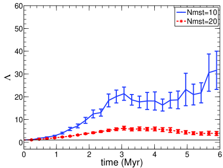
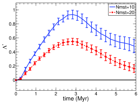
Figure 1: Evolution of the mass-segregation ratio for the 10 and 20 most massive stars (Nmst) using $\Lambda$ (left) and $\Lambda^{\prime}$ (right). The line $\Lambda=1$ (or $\Lambda^{\prime}=0$) represents the no-mass-segregation situation.

We use average $\Lambda$ and $\Lambda^{\prime}$ values for a given set of samples. Note that the average of $\log(\Lambda)$ is not equal to the logarithm of the average of $\Lambda$. The left-hand panel of Fig. 1 shows an increasing degree of mass segregation of the cluster with time from a very early stage. We also note that the dispersion of $\Lambda$ increases with time, which suggests that some $\Lambda$s may be extremely large, while others can be less than unity (i.e., the massive stars are less concentrated than the randomly selected sample stars). Therefore, if $\Lambda$ has a large dispersion, this may lead to an incorrect result, as we confirmed using $\Lambda^{\prime}$. There is a turnover point at approximately 3 Myr, shown in the right-hand panel of Fig. 1. That is, the cluster becomes more and more mass segregated until an age of 3 Myr and then the degree decreases. This turnover point may be related to our treatment of the escapers from the cluster. After truncating the cluster at a radius of 2.5 pc ($5r_{\rm v}$), we analyze the massive stars and the total number of member stars in the cluster.

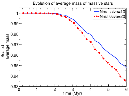
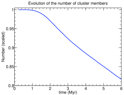
Figure 2: Evolution of the average mass of the 10 and 20 most massive stars (left) and the total number of stars in the cluster after truncating the cluster at a radius of $5r_{\rm v}$ (2.5 pc; right).

Fig. 2 shows the average mass of the 10 and 20 most massive stars and the total number left in the cluster as function of time. The average mass of the massive stars begins to decrease almost at the same time as the turnover point develops, while the cluster starts to lose members a little ($\leq 1$ Myr) earlier. When some of the massive stars leave the cluster, the MST length that includes these escapers becomes very large, leading to a relatively small value of $\Lambda^{\prime}$. This is the reason for the turning point in the $\Lambda^{\prime}$–$t$ curve. Therefore, we will radially truncate our clusters in the remainder of this paper.

3.2 Choice of velocity distribution

Because clumpy clusters evolve rapidly, small changes may significantly affect the results on short timescales. We find that the $\Lambda^{\prime}$ profile (as a function of time) changes if we vary the velocity distribution. In Fig. 3, we compare the results of the two different initial velocity distributions from Eq. (2). One is uniform throughout, while the other is radius dependent. For the radius-dependent velocity distribution, the degree of mass segregation reaches a peak at 0.5–1 Myr. Shortly thereafter, it drops to a relatively low level (similar to that of a uniform distribution). We will now attempt to offer an explanation for this behavior.

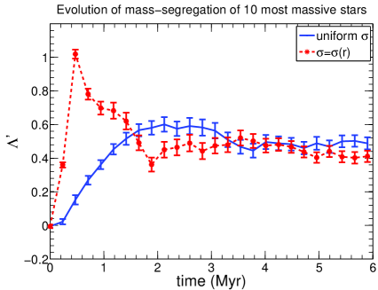
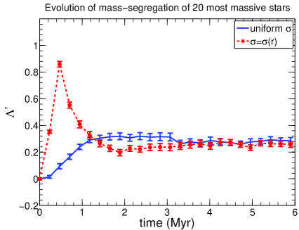
Figure 3: Evolution of the (left) 10 and (right) 20 most massive stars in the cluster for uniform and radius-dependent velocity dispersions.

We define the mean separation between stars using the MST length,

$$\langle l\rangle=\frac{\rm MST}{n-1},$$ (5)

where $n$ is the number of stars in the sample of interest. The mean separation of a sample of randomly selected stars in the cluster can be a trace of the mean separation within the cluster. Fig. 4 shows that the mean separation in the cluster and of the 10 most massive stars varies with time.

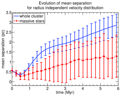
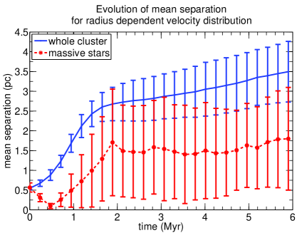
Figure 4: Evolution of the mean separation for (left) uniform and (right) radius-dependent velocity dispersions. The solid line is the mean separation in the entire cluster, while the dashed line represents the mean separation of the 10 most massive stars in the cluster.

It seems that for the radius-dependent velocity distribution, the curve of the mean separation of massive stars forms a valley at approximately 0.5 Myr, while the curve of the mean separation of the full cluster increases from the onset. This valley corresponds to core collapse of (only) the most massive stars in the cluster. A series of radii of different mass shells (increasing fractions of ‘most massive’ stars, from bottom to top) is presented in the left-hand panels of Fig. 5. The right-hand panels of Fig. 5 show increasing fractions of ‘inner cluster’ stars from bottom to top.

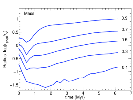
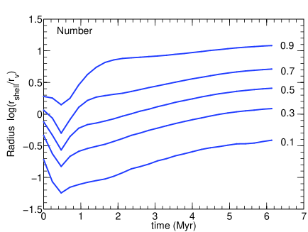
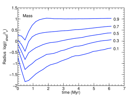
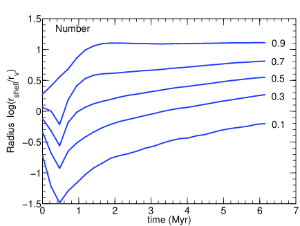
Figure 5: Evolution of (left) mass and (right) number shells for clusters truncated at $5r_{\rm v}$. The top and bottom panels are characterized by uniform and radius-dependent velocity dispersions, respectively. The numbers in the panels refer to the fractions (by number) of cluster stars included in the individual curves: the left-hand panels show increasing fractions of ‘most massive’ stars from bottom to top, while the right-hand panels show the equivalent behavior for increasing fractions of ‘inner cluster’ stars.

The evolution of the half-mass radius indicates that the cluster is undergoing a core-collapse process (driven by the most massive stars) until approximately 0.5 Myr, when it begins to re-expand. We compare this timescale to the crossing time, $t_{\rm cross}$, which is simply the cluster radius divided by its velocity dispersion. For our $N=1000,D=2.0$, and $q=0.30$ initial conditions, $t_{\rm cross}\sim 0.2$–0.6 Myr for the cluster as a whole. That is, core collapse of the few most massive stars happens during the first few crossing times. However, the crossing time for the core region depends on the adopted form for the radial velocity dispersion: it is 0.1–0.3 Myr for the uniform distribution and 0.08–0.2 Myr for the radius-dependent velocity dispersion.

For the radius-dependent velocity distribution, expansion of the outer parts of the cluster after formation can be traced from the evolution of the radius containing 90% (by number) of cluster stars. Therefore, the large $\Lambda^{\prime}$ seen at early times in Fig. 3 is caused by expansion of the cluster rather than by a concentration of the massive stars. This expansion is caused by the initially large velocity in the central parts. Therefore, the radius-dependent velocity dispersion would increase the velocity in the central part without changing the initial virial ratio. On the other hand, the evolution of the MST length of the cluster as a whole, which assigns all members of a sample equal weights, can also be a tool for measuring the size of the cluster.

3.3 Mass segregation in velocity space

The massive stars are becoming centrally concentrated very rapidly, thus leading to rapid dynamical mass segregation. On the other hand, stars of different masses may also exhibit different velocity dispersions. We adopt our MST method here to measure mass segregation in velocity-dispersion space. The only difference is that ‘distance’ now refers to the separation in velocity dispersion of two stars. Velocity dispersion is defined as

$$\mbox{\boldmath$\sigma$}_{i}={\bf v_{i}}-{\bf v},$$ (6)

where $\bm{\sigma}_{i}$ is the velocity dispersion of star $i$, ${\bf v}_{i}$ the velocity of star $i$, and ${\bf v}$ the velocity of the whole cluster. Therefore, the separation in velocity dispersion of two stars can be expressed as

$$\mbox{\boldmath$\sigma$}_{ij}=\mbox{\boldmath$\sigma$}_{i}-\mbox{\boldmath$\sigma$}_{j}={\bf v_{i}}-{\bf v_{j}},$$ (7)

which is same as separation in terms of velocities.

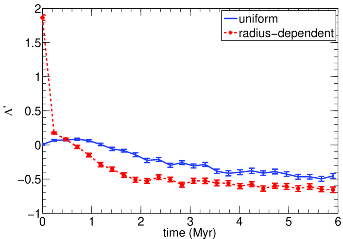
Figure 6: Evolution of mass segregation in velocity space. The solid and dashed lines represent mass segregation for a uniform, random velocity dispersion and for the radius-dependent dispersion, respectively.

From Fig. 6 we find that clusters can exhibit ‘inverse mass segregation’ in velocity space by calculating $\Lambda^{\prime}$ using the same treatment as before. The reason for this is that the massive stars are preferentially concentrated in the core and have a higher velocity dispersion than a sample of randomly selected stars.

4 Conclusions

We have presented simulations and analysis of the early evolution of initially cool and clumpy star clusters by performing a large number of $N$-body simulations. An MST method is used to measure the degree of mass segregation. In addition, it can also be a ruler to trace cluster size. Removal of the ejected stars is important physically, since it has an effect on measuring the cluster’s mass segregation.

We also conclude that the velocity distribution has an impact on mass segregation during core collapse. For a radius-dependent velocity distribution, which leads to a high velocity in the inner regions, the picture of (the dynamical evolution of) the cluster during the core-collapse period is very different from that resulting from the assumption of a constant velocity dispersion. Although the high-mass stars still undergo core collapse, the entire cluster expands from its formation epoch. As a result, a high degree of mass segregation results at the time of high-mass core collapse. We also adopt the MST method to discuss mass segregation in velocity space, finding ‘inverse mass segregation,’ which may be caused by the high velocity dispersion of the massive stars.

Because our aim in this paper was to explore the effects of a radially dependent velocity dispersion on early mass segregation, we have not included the effects of primordial binary stars (beyond their dynamical formation in our simulations). This is clearly an important omission, which we intend to address in our future work. A high initial binary fraction would introduce, on average, a higher velocity of escaping stars (Weidner et al., 2010), which is commonly seen in observations of young star clusters. However, Weidner et al. (2010) also found that the degree of mass loss is nearly independent of whether or not the cluster possesses primordial binaries. In addition, for a $N=1000$ cluster, varying the binary fraction within reasonable bounds has little effect on the mean mass of escapees. As a result, inclusion of initial binaries will likely not significantly affect the signature of mass segregation in our simulated clusters.

References

- Allison et al. (2009a) Allison R. J., Goodwin S. P., Parker R. J., de Grijs R., Portegies Zwart S. F., & Kouwenhoven M. B. N. 2009a, ApJ, 700, L99
- Allison et al. (2009b) Allison R. J., Goodwin S. P., Parker R. J., Portegies Zwart S. F., de Grijs R., & Kouwenhoven M. B. N. 2009b, MNRAS, 395, 1449
- Allison et al. (2010) Allison R. J., Goodwin S. P., Parker R. J., Portegies Zwart S. F., & de Grijs R. 2010, MNRAS, 407, 1098
- Ascenso et al (2009) Ascenso J., Alves J., & Lago M.T.V.T 2009, A&A, 495, 147
- Carpenter & Hodapp (2008) Carpenter J. & Hodapp K. 2008, in: Handbook of Star Forming Regions, Vol. I, p. 899
- Cartwright & Whitworth (2004) Cartwright A. & Whitworth A. P. 2004, MNRAS, 348, 589
- Chen et al. (2007) Chen L., de Grijs R., & Zhao J. L. 2007, AJ, 134, 1368
- Converse & Stahler (2010) Converse J. M., Stahler S. W. 2010, MNRAS, in press
- Elmegreen (2000) Elmegreen B. G. 2000, ApJ, 530, 277