Measuring Lensing Magnification of Quasars by Large Scale Structure using the Variability-Luminosity Relation

Abstract

We introduce a technique to measure gravitational lensing magnification using the variability of type I quasars. Quasars’ variability amplitudes and luminosities are tightly correlated, on average. Magnification due to gravitational lensing increases the quasars’ apparent luminosity, while leaving the variability amplitude unchanged. Therefore, the mean magnification of an ensemble of quasars can be measured through the mean shift in the variability-luminosity relation. As a proof of principle, we use this technique to measure the magnification of quasars spectroscopically identified in the Sloan Digital Sky Survey, due to gravitational lensing by galaxy clusters in the SDSS MaxBCG catalog. The Palomar-QUEST Variability Survey, reduced using the DeepSky pipeline, provides variability data for the sources. We measure the average quasar magnification as a function of scaled distance ($r/R_{200}$) from the nearest cluster; our measurements are consistent with expectations assuming NFW cluster profiles, particularly after accounting for the known uncertainty in the clusters’ centers. Variability-based lensing measurements are a valuable complement to shape-based techniques because their systematic errors are very different, and also because the variability measurements are amenable to photometric errors of a few percent and to depths seen in current wide-field surveys. Given the data volume expected from current and upcoming surveys, this new technique has the potential to be competitive with weak lensing shear measurements of large scale structure.

1. Introduction

Gravitational lensing of an object by mass along the line of sight produces two measurable effects: shape distortion and magnification of the source. It is usually impossible to measure the level of magnification since one typically does not know the intrinsic flux of the source. Because of this fundamental problem, the field of weak lensing has focused on shape measurements of sources since one can usually assume that galaxies have no preferred orientation. (For a review of gravitational lensing theory and techniques, see Schneider et al. 2004.) However, if the intrinsic luminosity of sources can be estimated, then lensing magnification can be used to study large scale structure.

Recently, large scale sky surveys have become efficient and prolific enough such that variability studies can be conducted on large samples of rare objects. For example, ensembles of type I (broad-line) quasars have been studied for the purpose of probing the physical causes of their common and dramatic variability (e.g., Vanden Berk et al. 2004, De Vries et al. 2005, Wilhite et al. 2008, Bauer et al. 2009b, Kelly et al. 2009, MacLeod et al. 2010, Meusinger et al. 2011). In these works, the mean ensemble variability amplitude has been seen to correlate with a number of properties of the objects: e.g., time scale of the variability, wavelength of observation, redshift, mass, and luminosity of the systems. In particular, a strong anti-correlation has repeatedly been observed between variability amplitude and quasar luminosity, particularly when comparing quasars of similar mass.

Given a measurement of a quasar’s variability amplitude, one can estimate its luminosity using this empirical relation. If the quasar were gravitationally lensed by intervening mass, the magnification effect would alter the observed luminosity. However, the fractional variability would remain unaffected, as the magnification, which is multiplicative on the luminosity, cancels. Therefore, magnification due to gravitational lensing will shift the quasar’s position in variability-luminosity space. Quantification of this shift constitutes a measurement of the quasar’s lensing magnification. Because the variability-luminosity relation has a large intrinsic variance, the estimate of a single quasar’s magnification is not precise. However, because the relation is well-determined in the mean, an ensemble of quasars can yield a significant measurement of the lensing effect.

In this paper we take advantage of the variability-luminosity relation seen in type I quasars to measure their magnification due to galaxy clusters along the line of sight. We use the Palomar-QUEST Variability Survey to measure the lensing magnifications of 3573 quasars, and compare the signal to that expected from gravitational lensing due to the 13,823 galaxy clusters in the Sloan Digital Sky Survey MaxBCG catalog (Koester et al. 2007). We measure an average cluster profile shape that is consistent with previous studies of the MaxBCG cluster catalog, showing that this method of measuring lensing magnification is indeed effective.

2. AGN Structure and Quasar Optical Variability

An active galactic nucleus (AGN) is typically described as having several prominent structural components. The central black hole is fed by an accretion disk, which radiates a continuum of flux primarily in the optical and UV bands. Offset from the plane of the disk exist clumps of gas which absorb the disk’s flux and reradiate it as broad emission lines (hence the name broad line region (BLR)). Emission from the disk and the BLR constitute the majority of the optical flux observed in type I quasars, which are the highly luminous AGN for which the observer has a direct line of sight to these two structures. (Type I quasars will hereafter be referred to simply as quasars.) The detailed geometry of the disk and BLR are not well understood; they may be part of one continuous structure (e.g. Nicastro et al. 2003, Elvis 2000, Lovegrove et al. 2010), but they traditionally are described as being distinct. A minority of quasars also show evidence of radio emission from a jet. The fraction of quasars that have strong radio emission (i.e. are radio loud) is uncertain; estimates range from roughly 5 to 25% (Zamfir et al., 2008). Jet emission can account for a portion of a quasar’s optical flux, but the fraction of optical flux that is jet-based depends strongly on the properties and orientation of the particular object.

Radio-loud quasars are on average more optically variable than radio-quiet quasars; in particular, their short-timescale variability is enhanced (e.g., Kelly et al. 2009). This distinction implies that the jet contributes to the optical variability in these systems, most likely due to the dissipation of shocks.

Not all quasar variability is due to jet physics; quasars with no evidence of a jet also exhibit significant flux variations. Sesar et al. (2007), using the Sloan Digital Sky Survey (SDSS), found that at least 90% of quasars are variable by at least 0.03 magnitudes on timescales of up to several years. The variability of individual nearby radio-quiet quasars (and their lower-luminosity counterparts, Seyfert I galaxies) have been studied in detail using the technique of reverberation mapping (e.g. Blandford & McKee 1982, Bentz et al. 2009): spectra of the AGN are regularly obtained, and the variability of the spectral features is measured as a function of time. Such monitoring has revealed that the disk continuum fluctuations are followed by fluctuations in the broad emission lines that echo the continuum variation. The time lag between the continuum and broad line variability constitutes a measurement of the BLR size, which is typically on the order of light-days. These measurements show that the primary source of variability in these objects is inside the BLR, presumably from the accretion disk and instabilities therein.

Accretion disk instabilities have long been a prime suspect as the main source of quasar variability. Kawaguchi et al. (1998) calculated the expected relationship between variability amplitude and timescale based on a model of disk instabilities, as well as a relation expected from starbursts in the quasar host galaxy. Hawkins (2002) extended this work to include a prediction based on microlensing of the quasars. A number of studies of ensemble quasar variability have measured the average variability amplitude versus timescale relation, which best agrees with the accretion disk instability calculation (Collier & Peterson 2001, Vanden Berk et al. 2004, De Vries et al. 2005, Wilhite et al. 2008, Rengstorf et al. 2006, Bauer et al. 2009b, Meusinger et al. 2011). However, this type of analysis would benefit from updated predictions using more complex models.

Disk instability models invoke relatively small, short-lived flares from numerous instabilities that combine to produce a stochastic light curve. These fluctuations could be prompted by changes in, for example, the accretion rate (e.g., Li & Cao 2008) or in a magnetic field (Hirose et al. 2009). Stochastic light curves have been succesfully used to describe optical observations of large samples of quasars (Kelly et al. 2009, Kozłowski et al. 2010, MacLeod et al. 2010). These works model the quasar light curves as a damped random walk, using only three parameters: the typical amplitude of the short-timescale variability, the damping timescale, and the average flux of the light curve. Such light curves, generated from a constant component plus similar flares with random start time, follow the variability-luminosity relation

$$\frac{\Delta L}{\overline{L}}\propto\overline{L}^{-\delta},$$ (1)

where $L$ is the object’s luminosity and $\delta$ depends on the details of the flares (Cid Fernandes et al. 1996, Cid Fernandes et al. 2000). Qualitatively, the anti-correlation simply notes that, given similar flare properties between two quasars, the fractional variability $\Delta L/\overline{L}$ will be smaller in the quasar whose mean luminosity $\overline{L}$ is larger. This prediction indeed describes the variability-luminosity anti-correlation seen in quasar ensembles (Vanden Berk et al. 2004, Bauer et al. 2009b).

Alternatively, it is possible that much of the observed relationship between variability and luminosity is a secondary effect of a correlation between, for example, variability and the quasar’s Eddington ratio. The Eddington ratio of a quasar describes its accretion rate, and can be estimated as a ratio between the quasar’s luminosity and its mass. Ai et al. (2010) find the correlation between Eddington ratio and variability to be more significant than that between luminosity and variability, using a sample of several hundred SDSS Seyfert I galaxies. The authors note the positive correlation between the accretion rate and the disk radius which emits at a given wavelength. Therefore an anti-correlation between variability amplitude and Eddington ratio implies that the outer regions of the disk show less variability than the inner radii (regardless of the physical mechanism behind the variability). This position-dependence qualitatively agrees with the observed anti-correlation between variability and wavelength (Wilhite et al. 2005), if the hotter, bluer, inner areas of the disk vary more strongly than the redder, outer regions. The variability amplitude may be anti-correlated with the quasar’s luminosity via such a positional dependence, and therefore through the definition of the Eddington ratio as related to the luminosity. As described in section 3, we normalize the quasar variability measurements according to the objects’ physical properties, including black hole mass. This procedure effectively allows us to measure how the variability amplitude scales with luminosity, for quasars of similar mass. Holding the mass constant in this way allows the variability-luminosity relation to contain the same information as the correlation between the variability and the Eddington ratio.

3. Measuring $\mu$

The average amplitude of quasar variability has been seen to depend on several factors: time lag between measurements, luminosity of the quasar (Vanden Berk et al. 2004, De Vries et al. 2005, Wilhite et al. 2008, Bauer et al. 2009b, MacLeod et al. 2010, Meusinger et al. 2011), wavelength of observation (Vanden Berk et al. 2004, De Vries et al. 2005, Meusinger et al. 2011), and black hole mass (Wilhite et al. 2008, Bauer et al. 2009b). The dependence of variability amplitude on redshift is less obvious; Vanden Berk et al. (2004) measured a slight increase in the variability with redshift, while De Vries et al. (2005) measured a slight decrease. More recently, MacLeod et al. (2010) and Meusinger et al. (2011) have measured no significant dependence of variability amplitude on redshift.

In practice, the variability-luminosity trend measured is of the form:

$$\log(V)=C-\alpha\times\log(L_{\mathrm{meas}}).$$ (2)

A linear relation has indeed been observed (Vanden Berk et al. 2004, Bauer et al. 2009b), although there are conflicting results for the value of the power-law slope $\alpha$, perhaps due to selection effects. If faint quasars are included in the analysis for which one cannot observe the full extent of the variability, the measured slope will become artificially shallow; this effect most clearly manifests itself as a flattening in the relation at the lowest observable luminosities, as is illustrated in figure 5 of Bauer et al. (2009b). The low-luminosity limit of the binning scheme in this work is chosen to exclude this regime from the data set. The value of the constant $C$ depends on the details of the normalization of the data, as described below.

When studying how the variability of a large quasar sample depends on one of the quasars’ properties, we must treat the parameters as independently as possible. To this end, we use a method introduced by Vanden Berk et al. (2004) and adopted in Bauer et al. (2009b). Four basic quantities are known for all of the quasars in our sample: time lag between measurements $\tau$, luminosity $L$, estimated black hole mass $M$, and redshift $z$. There are known correlations between all of these parameters, due to physical relationships or artificial effects such as detection biases in flux-limited surveys. To avoid these complications and study only the dependence of variability on luminosity, we would like to identify a set of quasars with identical properties except for their luminosity, and then examine how the variability differs between them. To approximate this procedure, we have split each parameter’s range into bins: 8 bins in $\tau$, 6 bins in $M$, 6 bins in $z$, and 4 bins in $L$. The bin limits are given in table 1; quasars with properties outside the given ranges are not used in the analysis.

$\tau$	$z$	$M$	$L$
1	0.40	1	30.85
5	0.80	4	31.05
10	1.10	8	31.20
20	1.40	12	31.40
60	1.65	20	31.50
130	1.90	30
160	2.20	75
220
400

Table 1Bin limits used in determining the normalization constants. Measurements with values outside the limits are not considered. Units of time lag $\tau$: days; black hole mass $M$: $10^{8}\times M_{\odot}$, luminosity $L$: $\frac{\mathrm{erg}}{\mathrm{s}\cdot\mathrm{Hz}}$.

To measure quasar variability we use a quantity similar to that of the structure function. We define:

$$V=\sqrt{(\Delta m)^{2}-\sigma^{2}},$$ (3)

where $\Delta m$ is the magnitude difference between two independent observations of an object, and $\sigma$ is the error on those measurements. This is similar to the structure function as used in Vanden Berk et al. (2004) and Bauer et al. (2009b); however, here instead of being an ensemble measurement, one $V$ is measured for each pair of magnitude measurements of a quasar. Four measurements of a quasar will yield six $\Delta m$ measurements, and therefore six different $V$ measurements for the single quasar. As $V$ is imaginary when $\Delta m$ is less than the measurement error $\sigma$, we only use data which show significant ($>1\sigma$) variability. This cut on the data is described further in section 5.1.

For each multi-dimensional bin, a mean variability amplitude $\overline{V}$ is determined by taking the mean of all $V$ values measured for that bin. Then, holding constant the indices for time lag, mass, redshift, and wavelength, one can compare the $\overline{V}$ values across the 4 $L$ bins. This procedure yields $8\times 6\times 6=288$ possible 4-point plots of mean variability amplitude $\overline{V}$ versus luminosity, or 1152 possible $\overline{V}$ values. Most of the multi-dimensional bins are not well populated by the quasar sample (for example, high-redshift low-luminosity bins). In fact, we obtain 403 bins with at least 50 measurement pairs, which is the minimum we require in order to adequately determine $\overline{V}$. To examine the overall behavior of $\overline{V}$ with respect to $L$ one can normalize the 4-point measured trends together and average the resulting normalized data in each $L$ bin to find a simple, meaningful result of how the variability scales with the quasar luminosity. The normalization consists of an additive constant in log($\overline{V}$), i.e. each 4-point measured trend has its own constant $C$ as defined in equation 2. The $\tau$, $M$, and $z$ multi-dimensional bin that has the best statistics is chosen to be the standard, and the log($\overline{V}$) versus log($L$) trends from all other $\tau$, $M$, and $z$ bins are normalized to that standard using one constant offset per $\tau$, $M$, $z$ combination. The constant is determined by minimizing the chi square difference between the $\overline{V}$ values from the two datasets in the same $L$ bin, for the $L$ bins where there exist data from both sets. For a visual representation of the normalization procedure, see figure 4 in Bauer et al. (2009b). After averaging the normalized data, we are left with one $V_{\mathrm{norm}}$ versus $L$ trend with arbitrary $y$ axis normalization but meaningful slope. This normalization technique has been shown to give results for variability amplitude versus time lag $\tau$ that are consistent with independent measurements (see table 4 in Bauer et al. (2009b). In this way, we study how the variability scales with luminosity, comparing only objects with similar values of the other parameters. After the normalization, deviations from the mean $V_{\mathrm{norm}}-L$ relation will not be caused by known, but lensing-independent, correlations such as that between variability and time lag. Using the normalization constants calculated in this way, each measured variability amplitude $V$ is normalized according to its $\tau$, $M$, and $z$ bin; the resulting $V_{\mathrm{norm}}$ then can be used to estimate the quasar’s lensing magnification, as detailed below.

We note that, for data taken in a single pass-band, the redshift of the quasar is degenerate with the rest-frame wavelength observed: the effective wavelength of the filter in the quasar’s rest frame scales as $(1+z)$. Because rest-frame wavelength of observation scales monotonically with redshift, these two variables are simultaneously accounted for in our normalization versus redshift.

When fitting for $\alpha$ and $C$ in equation 2 , we find the linear fit that best describes the whole quasar sample. On average, the measured luminosity $L_{\mathrm{meas}}$ of quasars in the sample is equal to $\overline{\mu}L_{\mathrm{intrinsic}}$, where $\overline{\mu}$ is a magnification value representative of the entire sample. We can therefore rewrite equation 2 as

$$\log(V_{\mathrm{norm}})=C-\alpha\times\log(\overline{\mu}L_{\mathrm{intrinsic}})$$ (4)

where we have also explicitly noted the fact that the $V$ measurements are normalized.

Once we have determined the unique constants $\alpha$ and $C$ for the whole data set, we can use a measured and normalized $V_{\mathrm{norm}}$ of a quasar to constrain $\overline{\mu}L_{\mathrm{intrinsic}}$ since equation 4 is equivalent to

$$\overline{\mu}L_{\mathrm{intrinsic}}=\left(\frac{10^{C}}{V_{\mathrm{norm}}}\right)^{1/\alpha}.$$ (5)

Qualitatively, we simply use the $V_{\mathrm{norm}}$ for a quasar to read off an expected value of $L_{\mathrm{meas}}$ from the linear $\log(\overline{V}_{\mathrm{norm}})-\log(L_{\mathrm{meas}})$ plot. This expected $L_{\mathrm{meas}}$, as it is the prediction calculated using the luminosities of the entire quasar sample, is an estimate of $\overline{\mu}L_{\mathrm{intrinsic}}$, where $L_{\mathrm{intrinsic}}$ is the intrinsic luminosity of that quasar. Comparing this value to a direct measurement of the luminosity of the quasar $L_{\mathrm{meas}}$, we can measure any shift in the luminosity, i.e. magnification or demagnification:

$$\frac{\mu_{\mathrm{true}}}{\overline{\mu}}\equiv\frac{L_{\mathrm{meas}}}{\overline{\mu}L_{\mathrm{intrinsic}}}=L_{\mathrm{meas}}\left(\frac{V_{\mathrm{norm}}}{10^{C}}\right)^{1/\alpha}.$$ (6)

We define $\mu^{\prime}\equiv\mu_{\mathrm{true}}/\overline{\mu}$, the relative magnification with respect to the typical value for the whole sample. For a large set of quasars taken from a broad sky area, such as the data used in this work, we expect $\overline{\mu}$ to be close to unity. In this way, each variability measurement $V$, calculated from a pair of magnitude measurements $\Delta m$, yields an estimate of the quasar’s relative magnification $\mu^{\prime}$.

4. Palomar-QUEST RG-610 Data Set

We measure the lensing magnification of quasars using the Palomar-QUEST Variability Survey. The survey used the QUESTII large area camera (Baltay et al. 2007), which comprises 112 CCDs with a pixel scale of 0.878”/pixel, with an overall field of view of 9.6 square degrees. The camera was mounted on the 48” Samuel Oschin Schmidt telescope at the Palomar Observatory, during which it aquired two main data sets. First completed was a 3.5 year multi-color survey covering 15,000 square degrees roughly four times in each of seven optical filters (Johnson UBRI and SDSS $riz$), with a depth of roughly mag 21 in the SDSS $r$ filter. These data have been used to study the variability of AGNs (Bauer et al. 2009b, Bauer et al. 2009a), to search for highly variable objects in both the archival data (Bauer et al. 2009c) and real-time data (Djorgovski et al. 2008), and to study brown dwarfs (Slesnick 2006b, Slesnick 2006a), among other phenomena. The multi-color survey was executed concurrently with a 5 year, 30,000 square degree survey which used a single broad, red, RG-610 filter, and reached a depth of about mag 19.5 in SDSS $r$ in each 60 second exposure (under dark sky conditions). The bandpass for the RG-610 filter (filter transmission times the QUEST CCD quantum efficiency) is shown in figure 1. The single-filter survey has been used as the discovery data for the Nearby Supernova Factory (Copin et al. 2006), as well as for searches for dwarf planets and other solar system bodies (Brown et al. 2005).

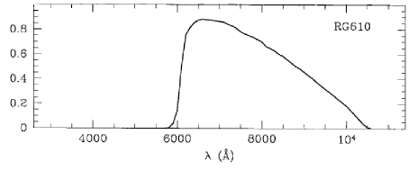
Figure 1.— RG-610 filter transmission, multiplied by CCD response.

This work uses the single-filter Palomar-QUEST data, and constitutes the first results from these data which rely on precision photometry. For this reason, we describe the DeepSky image reduction pipeline and the photometric calibration techniques which are used to generate flux measurements.

4.1. The DeepSky Image Reduction Pipeline

The Palomar-QUEST RG-610 data were taken by a variety of groups with different strategies, under different observing conditions, and with no uniform calibration procedure; daily operations in each of the groups emphasized simply discovering transients, rather than more precise photometry. Industry-standard reduction frames such as dark frames, dome flats, twilight flats, and fringe frames, were taken rarely or not at all. The DeepSky project has re-reduced these data using a standard pipeline designed to improve the precision of differential photometry, which we briefly describe below.

The DeepSky reduction suite treats each of the 112 CCDs in the QUESTII camera as a separate detector, attempting only to produce a uniform response on each frame rather than trying to flatten the detector response across the entire mosaic. Data frames for each stage of the reduction (dark, flat, etc.) were pooled for each month, and sometimes from several months in succession depending on what was available, to achieve the high statistics necessary to reject bad pixels and regions of the camera with unstable performance. The algorithms were cross-validated on subsamples of the data for months with many reduction frames, suggesting that the loss of performance is minimal when building reduction frames monthly rather than more frequently (weekly or daily). Each month about 100 calibration images from each chip were used to create ’superframes’ for the reduction.

Bias levels were first subtracted from each $600\times 2400$ pixel image using a $40\times 2400$ overscan region. Dark frames of different exposure times (10, 60, 100, and 240 sec) were combined, with the dark current $D_{i}$ at each pixel $i$ being fit to a model linear in the exposure time $t$: $D_{i}=a_{i}+b_{i}t$, where the ’instantaneous’ portion corresponds to dark current which accumulates during readout. Iterations of the fitting procedure rejected outlier values in determining the model parameters $a_{i}$ and $b_{i}$. Pixels for which no solution converged, or for which the “1 $\sigma$” interquantile width (median minus 16th percentile) of the distribution of residuals from the fit was more than three times wider than the median residual value for the image, were masked as bad pixels. All images were then corrected according to their exposure time using the superdark $D_{i}$.

In general neither twilight nor dome flats were regularly available, and images taken under dark-sky conditions were often contaminated with strong fringes. We therefore chose to construct flat fields using science images taken both during twilight and in moonlight. The calculations of Krisciunas & Schaefer (1991), appropriately adapted to Mt. Palomar, suggests that the loss of flatness due to the non-uniformity of moonlight should be less than 2% over the extent of each chip (0.5 degrees) for images taken more than 20 degrees from the moon, and we required this of images used to build the flat field. We also required that the sky level from scattered moonlight in these images be at least five times that typical of dark sky conditions. Images passing both of these cuts were normalized to a mean sky brightness of 1.0, and combined by taking the median at each pixel location to produce a superflat for the month. Pixels with unusually large fluctuations relative to other pixels were masked as bad, as for superdarks above. All images were then flattened using these superflats.

Superfringes were constructed in an analogous manner to the superflats using images taken under dark-sky conditions. The baseline fringe pattern was assumed to be a time-invariant characteristic of each chip over the month. The fringe amplitude in each science image was determined through cross-correlation with the superfringe, and the fringes in the image removed by subtracting the superfringe scaled by this amplitude. Changing sky conditions can of course produce time variations in the fringes, particularly in such a wide-band filter. We accept this as a systematic error in the photometry, with a contribution roughly on the same order as the sky noise under dark sky conditions.

Object detection and aperture photometry were performed on the detrended (bias-subtracted, dark-subtracted, flattened and de-fringed) images using SExtractor (Bertin & Arnouts 1996). Astrometry was performed on each frame using the astrometry.net suite (Lang et al. 2009). Magnitudes were measured for each object using ten aperture diameters ranging from 1 pixel to 16 pixels; this work uses the 3-pixel diameter aperture measurements as the primary flux measurement. Aperture corrections were calculated as the clipped median of the 12-pixel diameter aperture flux divided by the 3-pixel aperture flux. This correction was calculated using all good-quality measurements on a frame, and calculated separately for each frame.

4.2. Photometric Calibration

A number of cuts are made on the quality of the data. First, SExtractor flags are checked for objects that are blended or saturated, close to image boundaries, or for which the measurement failed; these flags eliminate about 3% of the data. A further saturation check is made by comparing object fluxes to saturation levels determined for each chip, which are more accurate than the single baseline saturation level checked by SExtractor. Very few objects are eliminated by this cut. Variations in the background sky level on the small spatial scale of 5$\times$5 pixels are examined, and a frame is discarded if they are typically large enough to contribute a 3% error to the photometry of an object with magnitude 18; this removes about 3% of the images. Frames are also rejected for which the median full width at half maximum (FWHM) exceeds 5 pixels, eliminating about 6% of the data. To ensure that closely spaced detections do not contaminate the aperture photometry, an object is rejected if it has a neighbor within four arc seconds ($\sim$3.5 pixels); most object affected by this cut are already discarded for being blended in SExtractor.

Spatial fluctuations of the moon/twilight flat fields and variability in night sky lines during observations made it difficult to completely remove the fringes from the data. This results in a $\sim 2\%$ flux systematic for bright objects, which is added in quadrature to the statistical errors.

A standard method of calibration is simply to determine a multiplicative constant zero point which corrects differences in average response (both intrinsic and weather-related) between two images. We perform such a frame-based calibration as a first step. All overlapping images are determined, and the one in which objects have the brightest measurements is assigned as the standard. A single zero point is determined for each frame in order to bring it to the level of the standard. This constant is determined using objects of all magnitudes. The correction is also calculated separately for bins of different magnitudes: five bins between SDSS r magnitudes of roughly 15 and 20. On average, the difference in the mean correction between the brightest bin and a fainter one ranges from about 3% to 6%. If a larger variation than this is seen, the frame is assumed to be non-linear and is not used. This eliminates about 15% of the data; the non-linearity is partially due to intrinsic properties of the CCDs, but primarily due to the insufficient quality of the fringe and flat field calibration data. Poor frames are also identified by comparing their measurements to the mean measurements of the objects they hold. If 15% of the flux measurements on a frame disagree with their objects’ means by more than 3 times the measurement errors, then the frame is discarded. This removes about 8% of the data, for which the systematic effects are catastrophic.

The systematic residuals in the data make a frame-based calibration insufficient for accurate photometry; while a systematic term describes the typical uncertainties, the error distribution is not Gaussian and therefore this procedure generates many photometric outliers. Because the spatial scale of the systematic variations is much larger than the size of each object, we can refine the frame-based calibration using an object-based one. This technique involves generating a zero point for one object at a time by considering only its close neighbors. A large scale systematic variation far away from an object will affect a frame-based calibration; an object-based one will be less sensitive to such features. We therefore implement, as a second step, an object-based calibration. We use the average of at least 10 neighbors within 150 arc seconds to calculate the correction between an object’s measurements on two scans. About 8% of the detections do not have enough neighbors to satisfy this requirement, and are therefore disregarded.

The frame calibration is calculated using only objects detected by the Sloan Digital Sky Survey (SDSS; Abazajian et al. 2009) and classified by them as pointlike. This precaution eliminates the possibility of our inadvertently using data artifacts, or galaxies which may exceed the aperture size, as calibration objects. For the purposes of this work, the object calibration is only performed on quasars which have been spectroscopically identified by SDSS. The reference objects used in the object calibration are limited to pointlike SDSS detections.

The strict cuts implemented in the photometric calibration throw away roughly 35% of the measurements. The systematic error is typically 2%, with about 3% of measurements disagreeing with the mean flux of the object by over 3 times their measurement errors. From previous variability studies we expect $<\sim$1% of measurements to be truly variable (Huber et al. 2006; Sesar et al. 2007); therefore, we infer that our photometry contains residual calibration errors in $\sim$2% of the measurements. Because in this work we deal only with the ensemble average over hundreds of measurements, and we expect the systematic error to be uncorrelated across different observations, we do not expect the residual errors to affect our results. Nonetheless, as a precaution against these errors we make additional cuts against variability behavior uncharacteristic of quasars; this is described further in section 5.1.

5. Results

We study a sample of 3573 spectroscopically identified quasars, spanning roughly 5,000 square degrees, from the SDSS data release 7. For each quasar we calculate its luminosity at 2500 Å by multiplying a redshifted composite quasar spectrum taken from Vanden Berk et al. (2001) with SDSS filter curves. We use the SDSS $z$ band magnitude, corrected for galactic extinction using the maps from Schlegel et al. (1998), to normalize the composite spectrum’s amplitude. We choose the $z$ band as it is least extincted by dust along the line of sight. We then take the normalized flux at 2500 Å  and convert it to luminosity using the object’s spectroscopic redshift and the cosmological parameters, which we assume to be $\Omega=1,\Omega_{\Lambda}=0.7,\Omega_{M}=0.3,H_{0}=0.71\frac{km}{s\cdot Mpc}.$ We also estimate the black hole mass for each quasar from the $M-\sigma$ relation, using the widths of the $\mathrm{H_{\beta}}$ and $\mathrm{Mg_{II}}$ emission lines as in Salviander et al. (2007), and calculating the radius of the BLR as described in Bentz et al. (2009).

In many cases during the Palomar-QUEST Survey, the same sky area was observed twice in the same night. Because quasars are not variable on such short timescales to the precision of our measurements, we average all intranight measurements to yield one flux value per night.

5.1. Data Cuts

As described above, we have made restrictions on the data quality in order to produce reliable photometry. Here we describe the criteria we use to select our quasar sample so that we have a well-measured, homogeneous dataset.

While the majority of quasar variability is thought to be due to accretion disk instabilities, some AGN show blazar characteristics, with considerable flux and variability from a jet component. Jet-based variability is much more dramatic than that seen in typical quasars, and because it is powered by shock dissipation and enhanced by relativistic beaming, it is not expected to follow the variability-luminosity relation seen in most quasars. It is therefore important to restrict the quasar list to those displaying variability that is characteristic of quasars.

We select quasars from SDSS that have the following properties:

1. spectroscopic identification in the SDSS, with a match to the spectral cross-correlation template number 29 (QSO) with confidence of at least 0.95

2. no detection in the FIRST (Becker et al., 1995) or RASS (Anderson et al., 2007) catalogs

3. redshift between 0.4 and 2.2

4. estimated black hole mass between $10^{8}\mathrm{M_{\odot}}$ and $7.5\times 10^{9}\mathrm{M_{\odot}}$

5. luminosity between $10^{30.85}\frac{\mathrm{erg}}{\mathrm{s}\cdot\mathrm{Hz}}$ and $10^{31.5}\frac{\mathrm{erg}}{\mathrm{s}\cdot\mathrm{Hz}}$.

Criteria 1 and 2 are meant to select radio-quiet AGN whose optical fluxes do not show significant contributions from a jet. Numbers 3-5 serve in part to crop the tails of the parameter distributions, and are the edges of the binning scheme that we use when normalizing the data as described below. The bin limits are stated again in table 1. The low redshift cut is chosen to eliminate objects that may appear spatially extended in the data, and therefore be poorly measured by the Palomar-QUEST photometry. The high redshift cut ensures that the quasar sample is selected homogeneously using UV-excess techniques. The low luminosity cut is chosen because for objects fainter than this level we see a flattening in the variability-luminosity relation, implying that these less luminous quasars vary to fluxes below our detection limit, causing us to not observe their full range of variability.

These criteria yield a sample of 4845 quasars that have Palomar-QUEST repeated measurements.

Furthermore, the quasars’ Palomar-QUEST measurements must satisfy:

1. $V\leq 0.1$ where $V$ is defined as in equation 3 and is calculated using all measurement pairs with rest-frame time lag less than 10 days

2. $V\leq 0.5$ where $V$ is defined as in equation 3 and is calculated using all measurement pairs with rest-frame time lag greater than 100 days.

These cut values are motivated by the variability amplitudes of quasars and blazars measured in Bauer et al. (2009a). Because the variability amplitude is unchanged for lensed and unlensed objects, this is an unbiased cut with respect to lensing analyses. This step eliminates 967 objects, leaving 3878 quasars. We note that this cut eliminates a much larger fraction of the AGN than is expected from the relative numbers of known blazars and quasars. However, the cut is not only sensitive to jet-based variability but also calibration errors, and is a strict but important criterion to ensure that poor quality measurements do not overwhelm the lensing signal. These 3878 quasars have, in total, 230,674 Palomar-QUEST measurement pairs.

We only use measurement pairs for which:

1. the rest frame time lag between measurements is shorter than 400 days

2. the measurements show significant ($>1\sigma$) variability

3. the variability amplitude is less than 1 magnitude

4. no more than 40 measurement pairs from each quasar are included.

Cut 1 eliminates a long but low-level tail out to larger time lags, and throws away 19,523 pairs. Cut 2 is necessary to avoid the calculation of imaginary $V$ values for individual measurement pairs and is very restrictive because the Palomar-QUEST systematic error is of the order of typical quasar variability amplitudes over rest frame timescales of weeks. Still, as will be seen in figure 2, the data after this cut continue to follow a variability-luminosity relation described by equation 2, and therefore can be used to measure magnification using equation 6. We also note that removing the lowest signal-to-noise $V$ values reduces error due to imprecise determination of the survey’s systematic uncertainties, given the dependence of $V$ on the measurement uncertainty as stated in equation 3. Because the systematic uncertainties stem in part from imperfect flat field and fringe calibration images, they can be time and position dependent and therefore difficult to determine precisely for each measurement. This cut eliminates 134,745 pairs.

Cut 3 is a final check against outliers that are uncharacteristic of quasar behavior, and only throws away 17 measurement pairs. Cut 4 serves to keep a minority of exceptionally well-measured quasars from dominating the dataset, since the number of measurement pairs rises as the number of measurements squared. This cut removes 14,671 pairs.

Normalization of the quasars, described in section 3, is only done if there are sufficient quasars with similar properties so that we can determine accurate zero points. We require 50 measurement pairs per $\tau$ $M$ $z$ $L$ bin, which removes 4359 measurement pairs.

We are left with 57,359 useable measurement pairs, from 3573 quasars. We note that many of our cuts are due to properties of the data such as statistics and measurement errors, rather than properties of the quasars. Cuts on future quasar data sets may not need to be so restrictive.

5.2. Variability-Luminosity Relation

After normalizing the data as described in section 3, we plot the normalized variability vs. luminosity relation, which is shown in figure 2. The $y$ axis error bars on the points are errors on the mean calculated from the spread of the measurements in each bin. The bins in the figure are smaller than those used in the normalization, in order to show the relation in more detail. The trend is indeed well-described by a power law, with index $\alpha=0.565\pm 0.007$. The best fit line is shown on the plot. This slope is steeper than that found in other works (e.g., Vanden Berk et al. 2004, Bauer et al. 2009b); however, it is not directly comparable since we only consider measurements for which we observe significant variability.

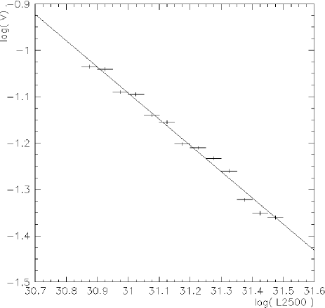
Figure 2.— Log Variability vs. Log Luminosity at 2500Å, after normalizations, determined using 57,359 measurement pairs. The best-fit line is shown, with slope $-0.565\pm 0.007$.

The precision of our magnification measurements relies on a narrow spread in the variability-luminosity relation. The residuals in log($V$) around the best-fit line are distributed normally, with a standard deviation $\sigma=0.22$ that is constant across our range of luminosity. These residuals are larger than the typical measurement errors, and therefore reflect an inherent spread in the quasar variability properties. There are several possible sources of the enhanced variance.

The measurement error on the luminosity is small, and is based simply on the uncertainties in the SDSS broadband magnitudes. This error estimate ignores the fact that the quasars vary by more than these uncertainties; the true mean luminosity could be tens of percent different from what was measured when the SDSS made its photometric observation. Since the spectroscopic quasar sample is much brighter than the SDSS photometric detection limit, there should be no Malmquist bias in the quasar sample and the error on the measured luminosity should be unbiased. Therefore, when discussing the variance of the relation, we assume that the luminosity is correct and simply absorb its error into the $y$ axis spread in values. In future studies this uncertainty can be reduced in cases where there are more photometric measurements per quasar, which can be averaged to produce a more accurate typical luminosity. (This is not possible with the Palomar-QUEST data, as it is relatively calibrated rather than absolutely.) Or, if many measurements are available, a lightcurve may be fit to each quasar’s data to determine the object’s baseline luminosity most accurately (see, e.g., MacLeod et al., 2010).

If the spread in the variability-luminosity relation is due to an effect with zero bias, then all quasars will intrinsically lie on the mean relation and increased statistics for a given object will move it closer to the mean trend. If quasars in the sample have heterogeneous variability properties, an object may lie intrinsically off the variability-luminosity relation and more statistics will only reveal this property more clearly. Some insight into this issue is given in MacLeod et al. (2008), which explores the implications of using many, as opposed to simply two, measurements of each quasar when studying the objects’ variability properties. They note that using only two measurements yields ensemble variability results similar to those determined using many epochs from the SDSS stripe 82 region. However, they also point out that there is an intrinsic spread in the quasars’ variability behavior that is not currently understood. This intrinsic difference between individual objects surely contributes to the scatter observed in the variability-luminosity relation, and is our motivation for including no more than 40 measurement pairs from each object in this analysis. More insight into the physical processes driving the different variability properties of individual quasars would help in understanding and reducing the systematic errors in the lensing magnification measurement.

Assuming statistically identical quasar lightcurves with power law spectra, Bauer et al. (2009b) used Monte Carlo simulations to show that using few measurements per quasar to calculate $V$ versus $\tau$ gives a slope that is unbiased, although windowing effects can make the trend non-linear at very short and long time lags (which are excluded from the data set in this work). Therefore we expect no significant bias to be introduced in this analysis due to the behavior of $V$ in the presence of sparse data sampling.

5.3. Magnification Measurements

Now that we have calibrated the quasar measurements and confirmed the variability-luminosity relation, we calculate the magnification $\mu^{\prime}\equiv\mu_{\mathrm{true}}/\overline{\mu}$ as defined in equation 6. The distribution of $\log(\mu^{\prime})$, with one entry per quasar measurement pair, is shown in figure 3. The distribution is wide and close to Gaussian. This is due to the distribution of the residuals of the $V-L$ relation, which has a similar shape. Because the scatter in the $V-L$ relation is large, the width of the $\log(\mu^{\prime})$ distribution is much wider than the range of magnifications expected in the data. Just as the mean of many variability measurements produces a precise variability-luminosity relation, the mean of many magnification measurements produces a meaningful result, with an error on the mean much smaller than the width of the distribution.

In order to obtain mean magnifications, we must bin the measurements in a physical quantity which we believe to be related to the magnification. Here we choose to bin the measurements in terms of their distance perpendicular to the line of sight (scaled as distance/$R_{200}$) from the nearest member of the MaxBCG galaxy cluster catalog.

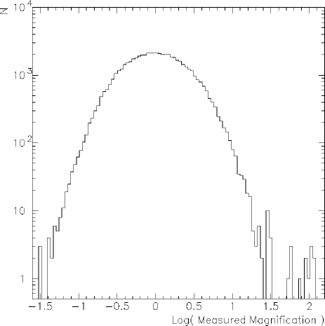
Figure 3.— Logarithm of the measured quasar magnifications, determined using 57,359 measurement pairs.

5.4. The Expected Signal

The strongest magnification of quasars is expected to be due to clusters of galaxies along the line of sight. To estimate the level of magnification that we expect quasars to experience, we can calculate the magnification due to the members of known cluster catalogs. For this purpose we use the MaxBCG catalog, which contains 13,823 clusters and covers about 7,500 square degrees. The MaxBCG catalog is estimated to be 90% pure and 85% complete for clusters between redshifts 0.1 and 0.3 and with masses greater than $10^{14}M_{\odot}$ (Koester et al., 2007). By adopting a model for each cluster, we can calculate the expected magnification of each quasar due to the galaxy clusters in the catalog.

We assign a Navarro-Frenk-White (NFW) profile (Navarro et al. 1997) to each cluster:

$$\rho(r)=\frac{\delta_{c}\rho_{\mathrm{crit}}}{(r/r_{s})[1+(r/r_{s})]^{2}}$$ (7)

where $c$ is the concentration parameter of the profile, $\delta_{c}=\frac{200}{3}\frac{c^{3}}{\mathrm{ln}(1+c)-c/(1+c)}$, $r_{s}=R_{200}/c$, and $R_{200}$ is the radius inside which the density is 200 $\times\rho_{\mathrm{crit}}$, the critical density of the universe at the redshift of the cluster. The total mass inside $R_{200}$ is $M_{200}$. We assume the cluster mass-richness relation used by Rozo et al. (2009):

$$M_{200}(N_{200})=\frac{1}{1.022}e^{0.48}\times\left(\frac{N_{200}}{20}\right)^{1.13}$$ (8)

to estimate $M_{200}$ given the richness $N_{200}$ stated in the cluster catalog. $M_{200}$ and $c$ have been seen to correlate with each other; we use the mass-concentration relation from Duffy et al. (2008):

$$c(M_{200},z)=5.71\times\left(\frac{M_{200}}{2.e12\times h^{-1}}\right)^{-0.084}\times(1+z)^{-0.47}$$ (9)

to determine $c$ given $M_{200}$ and the cluster redshift $z$. When calculating the magnifications, we truncate each profile at $3\times R_{200}$. If a quasar is close to more than one cluster, we multiply the magnifications due to each nearby cluster to produce a magnification estimate that includes contributions from all known clusters. Multiple magnifications are a minor effect; only 6.5% of the quasars have expected magnifications of $>1\%$ from more than one cluster.

A histogram of the logarithm of the predicted magnifications for the quasar sample is shown in figure 4. We predict one magnification per quasar, but we measure one $\mu^{\prime}$ per pair of magnitude measurements. The thick-lined histogram in figure 4 shows the distribution of magnification predictions, with one entry per quasar and therefore 3,573 entries. The thin-lined histogram includes one entry for each magnitude measurement pair: if a quasar has $N$ measurements, then that quasar’s predicted magnification will have $N(N-1)/2$ entries of identical value. The thin histogram therefore has 57,359 entries and is comparable to figure 3. The vast majority of the quasars are not significantly magnified by the clusters; however, there is a small tail of highly magnified objects up to $\mu\sim 2$. The striking difference in the shapes of the expected magnification distribution (figure 4) and the measured distribution (figure 3) is due to the large scatter in the individual measured values, reflecting the scatter in the $V-L$ relation. These figures visually demonstrate the need to average many magnification measurements in order to obtain a result precise enough to compare to theory/models.

The transverse distance between each quasar and the MaxBCG cluster closest on the plane of the sky is shown in figure 5; panel (a) shows the distance in the logarithm of kiloparsecs at the redshift of the closest cluster, while panel (b) shows the distance as a fraction of $R_{200}$ of the closest cluster.

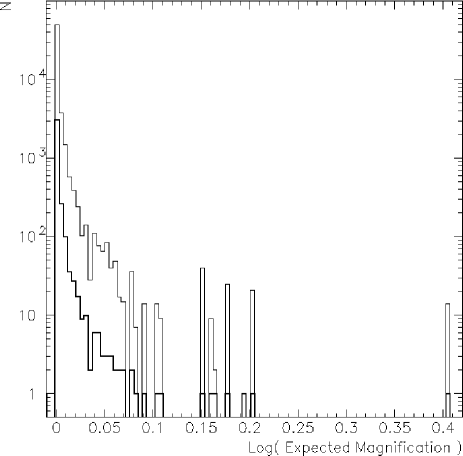
Figure 4.— Logarithm of the lensing magnification of quasars assuming NFW profiles for MaxBCG galaxy clusters. The thick-lined histogram includes one entry for each of the 3573 quasars which overlap the MaxBCG area. The thin-lined histogram shows the same calculated magnifications, but includes one entry for each of the 57,359 quasar measurement pairs and is therefore comparable to figure 3.

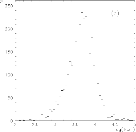
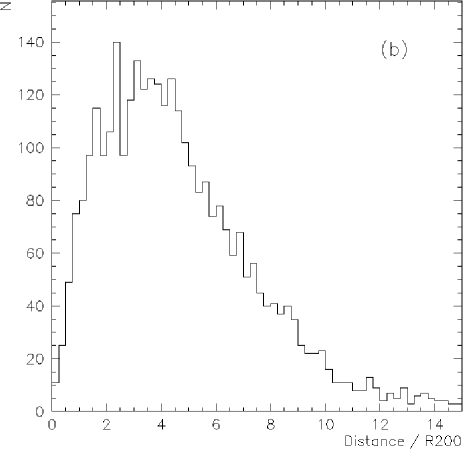
Figure 5.— Distance, transverse to the line of sight at the redshift of the cluster, between the quasars and the clusters which are closest on the plane of the sky. (a) in units of log kiloparsecs at the redshift of the cluster. (b) in units of $R_{200}$ of the closest cluster.

5.5. Magnification profile of the MaxBCG Clusters

For each quasar, we calculate the magnification we expect due to clusters in the MaxBCG catalog, as described in section 5.4. We then group the quasars in logarithmically spaced bins given by the quasar’s distance from the closest cluster, in units of $R_{200}$ of that cluster. The errors on the measurement are determined through bootstrap resampling. In particular, for each bin 1000 mean magnifications are calculated using random sampling with replacement such that the randomized set includes the same number of measurements as the original bin. The errors are taken to be the $1\sigma$ (15.9 and 84.1 percentile) values of the 1000 mean magnifications. Because the errors on the magnifications are in part caused by systematic uncertainties that are not currently understood, we prefer to derive the errors empirically in this way using the properties of the distribution itself.

Figure 6 shows the mean measured $\mu^{\prime}$ (points with error bars) and the expected magnification (points without errors, connected by lines), assuming NFW haloes for the MaxBCG catalog’s clusters as described above. While the magnification is significant and does fall with radius, we measure a systematically different magnification profile from that expected. The measured values compare to the expected magnifications with reduced $\chi^{2}=1.84$.

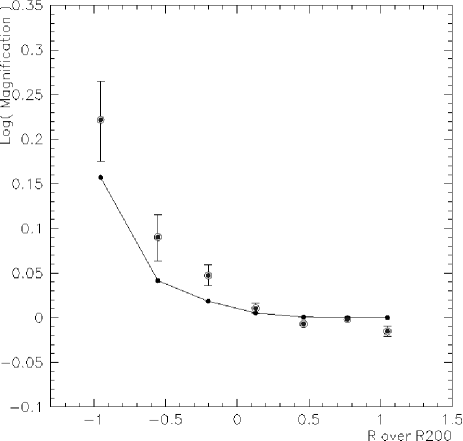
Figure 6.— Measured $\mu^{\prime}$ (points with error bars) and expected $\mu$ (points connected by lines), versus distance from the nearest cluster in units of $R_{200}$, assuming NFW profiles truncated at $3\times R_{200}$.

The MaxBCG catalog’s cluster positions are given as the location of the brightest cluster galaxy (BCG). This position does not always coincide with the center of the dark matter halo. Errors in the cluster central coordinates cause the average radial profile of the MaxBCG clusters (as measured from the reported centers) to differ from NFW. Johnston et al. (2007) studied this effect using weak lensing shear measurements and N-body simulations, and found a Gaussian distribution of positional offsets between the true and measured centers, with a richness-dependent probability that the cluster is correctly centered. To determine the effects of such offsets on our expected magnifications we implement the prescription of Johnston et al. (2007), offsetting the center of a subset of the clusters in a random manner. The results are shown in figure 7, and provide an improved fit to the data, with reduced $\chi^{2}=1.17$. The agreement between the data and predictions may be further improved by modelling the effects of large scale structure outside the redshift range of the MaxBCG catalog; however, these effects are subdominant and beyond the scope of this paper.

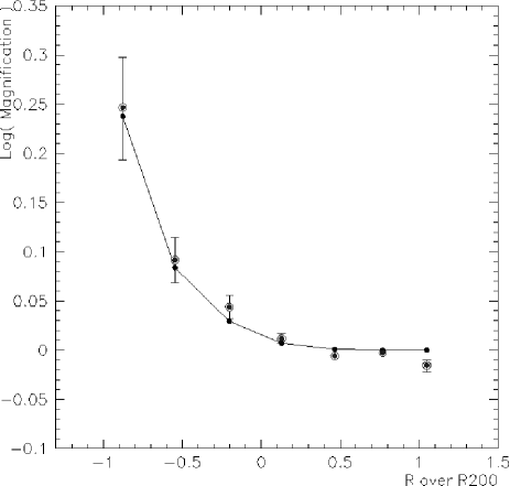
Figure 7.— Measured $\mu^{\prime}$ (points with error bars) and expected $\mu$ (points connected by lines), versus distance from the nearest cluster in units of $R_{200}$, assuming NFW profiles truncated at $3\times R_{200}$ and with centers offset as prescribed in Johnston et al. (2007).

Using the errors on the binned measurements determined through bootstrap resampling, we can estimate the error on each magnification measurement. Figure 8 shows the logarithm of the error on each bin versus the number of measurements in that bin, taken from the data in figure 7, with a best-fit line superimposed. The trend falls as $\sqrt{N}$, and at the level of our most populated bin (with 21,482 measurement pairs) shows no sign of a systematic floor. The best-fit line extrapolates to imply that each $\mathrm{log}(\mu^{\prime})$ measurement, made using one magnitude measurement pair, has an error of roughly 0.4. For a magnification of 1.1, this corresponds roughly to a signal to noise of 1 for each magnification measurement.

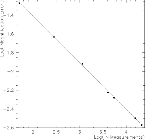
Figure 8.— Logarithm of the error on each bin versus the number of measurements in that bin, taken from the data in figure 7, with a best-fit line superimposed. The trend falls as $\sqrt{N}$, implying an error on $\mathrm{log}(\mu^{\prime})$ of 0.04 for a magnification measurement using one pair of magnitude measurements.

6. Discussion and Conclusions

We introduce a new technique to measure the effects of gravitational lensing by large scale structure. Type I quasars on average follow a well-constrained variability-luminosity relation; lensing magnification causes a significant shift in this relation. We describe the magnification measurement procedure, and use it to determine the magnification of background quasars due to lensing by the galaxy clusters in the MaxBCG catalog.

The measured magnification is significant, and consistent with the signal expected from the catalog. In particular, the agreement between the data and expectations is improved when the miscentering of the clusters is taken into account, as described in Johnston et al. (2007), compared to when the clusters are assumed to be NFW profiles centered exactly on their catalog positions. The lensing effects of the MaxBCG catalog have been measured very precisely using weak lensing shear, for example in Sheldon et al. (2009). Although the magnification measurements presented here are not competitive with such results, they serve to show that quasar variability can be used to study lensing magnification, and are the first measurements using this new technique.

Using quasar variability to measure gravitational magnification is a very different approach from the common method of using galaxy shapes to measure gravitational shear. Precision shape measurements of distant galaxies require very good quality data with faint flux limits and small point spread functions. Furthermore, the complex intrinsic shapes of galaxies make the shear measurement nontrivial. Measuring the variability amplitudes of quasars is much more simple, as these objects are often bright and they typically vary by amounts larger than the photometric errors of surveys such as Palomar-QUEST or SDSS. We see the error on the measured magnification to be roughly given by

$$\log(\sigma_{\log\mu})=-0.5\log(N_{\Delta m})-0.4$$ (10)

where $N_{\Delta m}$ is the number of $\Delta m$ measurements. This can be compared to the error on weak lensing measurements of the reduced shear $g$, which scale as $\sigma_{g}=\sigma_{\epsilon}\times(1-|g|^{2})/\sqrt{N_{\mathrm{gal}}}\approx\sigma_{\epsilon}/\sqrt{N_{\mathrm{gal}}}$ for moderate shears. The intrinsic scatter in the galaxy shapes is $\sigma_{\epsilon}\sim 0.35$ (Schneider et al. 2004), and $N_{\mathrm{gal}}$ is the number of measured galaxies. For magnification by a galaxy cluster with an NFW profile parameterized by $M_{200}=10^{14}$ and concentration $c=6$, a region with moderate magnification $\mu=1.05$ would have reduced shear $g=0.035$. In this regime, 100 galaxies and 100 $\Delta m$ measurements would yield signal to noise $S/N_{\mu}$ = 10 and $S/N_{g}$ = 1. A region of higher magnification $\mu$ = 1.25 and $g$ = 0.083 would yield again $S/N_{\mu}$ = 10, with $S/N_{g}$ = 2.4. This lensing strength is at the upper end of the range for which weak lensing techniques have been rigorously tested, for example by the STEP2 project (Massey et al. 2007). Stronger distortions are not straightforward to measure, particularly using the common KSB method (Kaiser et al. 1995). The variability-based quasar magnification analysis, on the other hand, is equally applicable to all lensing regimes.

The fact that the magnification measurements each have higher signal to noise than the shear measurements is offset by the relative sparsity of quasars compared to inactive galaxies. In the current SDSS spectroscopic sample, which reaches depths of $r$ $\sim$ 19.5, there are about 15 quasars per square degree. In data down to $r$ $\sim$ 20.5 we expect roughly 40 quasars per square degree (Richards et al. 2006). This depth will soon be available over large areas of sky. For example, BOSS is expected to double the number of spectroscopic quasars in the SDSS Survey over the next several years, over a footprint of 10,000 square degrees. Shear analyses are usually performed over much smaller areas of high quality data. For example, results from the CFHT Wide Survey use 50,000 galaxies per square degree, down to a magnitude of $i$ $\sim$ 24.5, with a total area of 34 square degrees (Fu et al. 2008). In order to reach the same signal to noise for moderate lensing strengths of $\mu=1.05$ and $g=0.035$, assuming 40 quasars and 50,000 galaxies per square degree, we would need fewer than 4 magnitude measurements on average for each quasar (assuming that the measurements give uncorrelated information about the magnification; more work is required to investigate this systematic complication). Assuming shallower data with 15 quasars per square degree, we would require 6 magnitude measurements of each quasar, on average, over just 34 square degrees. Alternatively, the same signal to noise could be achieved with just 2 measurements per quasar over an area of 1100 square degrees. These levels of data are easily obtainable with surveys such as BOSS and Pan-STARRS, which will provide $>$10,000 square degrees with sufficient data quality for magnification measurements. This is in sharp contrast with the $\sim 70$ square degrees which will be available from Pan-STARRS Medium Deep fields with the quality assumed here for shear measurements.

This work introduces the technique of using variability to measure the lensing magnification of quasars, and measures the magnification of 3573 quasars, with magnitudes down to SDSS r $\sim$ 19.5, due to lensing by known galaxy clusters along the line of sight. Future large-area sky surveys will be able to apply this new technique to measure lensing magnification over larger volumes, and improve our understanding of large scale structure.

References

- Abazajian et al. (2009) Abazajian, K. N., et al. 2009, ApJS, 182, 543
- Ai et al. (2010) Ai, Y. L., Yuan, W., Zhou, H. Y., Wang, T. G., Dong, X., Wang, J. G., & Lu, H. L. 2010, ApJL, 716, L31
- Anderson et al. (2007) Anderson, S., et al. 2007, AJ, 133, 313
- Baltay et al. (2007) Baltay, C., et al. 2007, PASP, 119, 1278
- Bauer et al. (2009a) Bauer, A., Baltay, C., Coppi, P., Ellman, N., Jerke, J., Rabinowitz, D., & Scalzo, R. 2009a, ApJ, 699, 1732
- Bauer et al. (2009b) —. 2009b, ApJ, 696, 1241
- Bauer et al. (2009c) Bauer, A., et al. 2009c, ApJ, 705, 46
- Becker et al. (1995) Becker, R., White, R., & Helfand, D. 1995, ApJ, 450, 559
- Bentz et al. (2009) Bentz, M. C., Peterson, B. M., Netzer, H., Pogge, R. W., & Vestergaard, M. 2009, ApJ, 697, 160
- Bertin & Arnouts (1996) Bertin, E., & Arnouts, S. 1996, A&AS, 117, 393
- Blandford & McKee (1982) Blandford, R. D., & McKee, C. F. 1982, ApJ, 255, 419
- Brown et al. (2005) Brown, M., et al. 2005, AJ, 635, L97
- Cid Fernandes et al. (2000) Cid Fernandes, R., Sodré, L., & Vieira de Silva, L. 2000, ApJ, 544, 123
- Cid Fernandes et al. (1996) Cid Fernandes, Jr., R., Aretxaga, I., & Terlevich, R. 1996, MNRAS, 282, 1191
- Collier & Peterson (2001) Collier, S., & Peterson, B. 2001, ApJ, 555, 775
- Copin et al. (2006) Copin, Y., et al. 2006, New Astronomy Review, 50, 436
- De Vries et al. (2005) De Vries, W., et al. 2005, AJ, 129, 615
- Djorgovski et al. (2008) Djorgovski, S. G., et al. 2008, Astronomische Nachrichten, 329, 263
- Duffy et al. (2008) Duffy, A. R., Schaye, J., Kay, S. T., & Dalla Vecchia, C. 2008, MNRAS, 390, L64
- Elvis (2000) Elvis, M. 2000, ApJ, 545, 63
- Fu et al. (2008) Fu, L., et al. 2008, A&A, 479, 9
- Hawkins (2002) Hawkins, M. 2002, MNRAS, 329, 76
- Hirose et al. (2009) Hirose, S., Krolik, J. H., & Blaes, O. 2009, ApJ, 691, 16
- Huber et al. (2006) Huber, M. E., Everett, M. E., & Howell, S. B. 2006, AJ, 132, 633
- Johnston et al. (2007) Johnston, D. E., et al. 2007, ArXiv e-prints
- Kaiser et al. (1995) Kaiser, N., Squires, G., & Broadhurst, T. 1995, ApJ, 449, 460
- Kawaguchi et al. (1998) Kawaguchi, T., et al. 1998, ApJ, 504, 671
- Kelly et al. (2009) Kelly, B. C., Bechtold, J., & Siemiginowska, A. 2009, ApJ, 698, 895
- Koester et al. (2007) Koester, B. P., et al. 2007, ApJ, 660, 239
- Kozłowski et al. (2010) Kozłowski, S., et al. 2010, ApJ, 708, 927
- Krisciunas & Schaefer (1991) Krisciunas, K., & Schaefer, B. E. 1991, PASP, 103, 1033
- Lang et al. (2009) Lang, D., Hogg, D. W., Mierle, K., Blanton, M., & Roweis, S. 2009, ArXiv e-prints
- Li & Cao (2008) Li, S., & Cao, X. 2008, MNRAS, 387, L41
- Lovegrove et al. (2010) Lovegrove, J., Schild, R. E., & Leiter, D. 2010, ArXiv e-prints
- MacLeod et al. (2008) MacLeod, C., Ivezić, Ž., de Vries, W., Sesar, B., & Becker, A. 2008, in American Institute of Physics Conference Series, Vol. 1082, American Institute of Physics Conference Series, ed. C. A. L. Bailer-Jones, 282–286
- MacLeod et al. (2010) MacLeod, C. L., et al. 2010, ArXiv e-prints
- Massey et al. (2007) Massey, R., et al. 2007, MNRAS, 376, 13
- Meusinger et al. (2011) Meusinger, H., Hinze, A., & de Hoon, A. 2011, A&A, 525, A37+
- Navarro et al. (1997) Navarro, J. F., Frenk, C. S., & White, S. D. M. 1997, ApJ, 490, 493
- Nicastro et al. (2003) Nicastro, F., Martocchia, A., & Matt, G. 2003, ApJL, 589, L13
- Rengstorf et al. (2006) Rengstorf, A., Brunner, R., & Wilhite, B. 2006, AJ, 131, 1923
- Richards et al. (2006) Richards, G. T., et al. 2006, AJ, 131, 2766
- Rozo et al. (2009) Rozo, E., et al. 2009, ApJ, 699, 768
- Salviander et al. (2007) Salviander, S., et al. 2007, ApJ, 662, 131
- Schlegel et al. (1998) Schlegel, D., Finkbeiner, D., & Davis, M. 1998, ApJ, 500, 525
- Schneider et al. (2004) Schneider, P., Kochanek, C., & Wambsganss, J. 2004, Saas-Fee Advanced Courses, Vol. 33, Gravitational Lensing: Strong, Weak and Micro, ed. G. Meylan, P. Jetzer, & P. North (Berlin, Germany; New York, U.S.A.: Springer)
- Sesar et al. (2007) Sesar, B., et al. 2007, AJ, 134, 2236
- Sheldon et al. (2009) Sheldon, E. S., et al. 2009, ApJ, 703, 2217
- Slesnick (2006a) Slesnick, C. e. a. 2006a, AJ, 131, 2665S
- Slesnick (2006b) —. 2006b, AJ, 131, 3016S
- Vanden Berk et al. (2001) Vanden Berk, D., et al. 2001, AJ, 122, 549
- Vanden Berk et al. (2004) —. 2004, ApJ, 601, 692
- Wilhite et al. (2005) Wilhite, B., et al. 2005, ApJ, 633, 638
- Wilhite et al. (2008) —. 2008, MNRAS, 383, 1232
- Zamfir et al. (2008) Zamfir, S., Sulentic, J. W., & Marziani, P. 2008, MNRAS, 387, 856