Joint density of states and its relationship with quasiparticle interference pattern in $d$-wave superconductors

Abstract

We present analytic analyses of the joint density of states (JDOS) and the elastic scattering susceptibility (ESS) for $d$-wave superconductors under the linear dispersion approximation. The JDOS and ESS diverge on the same curves which are found to be the envelope functions related to the contour of constant energy of the Bogoliubov quasiparticles. The relative amplitudes of the divergence on the envelope functions are derived. It is also found that certain octet vectors come close to the vertices of the envelope curves when the Dirac-cone anisotropy is strong, which is relevant to the $d$-wave cuprates.

The scanning tunneling spectroscopy(STS) has long been applied to exploration of the local single-particle spectrum of high-$T_{c}$ cuprates  Fischer . Recently, modulations of the local density of states (LDOS) have been studied by the Fourier transformed (FT) STS and analyzed within the quasiparticle interference (QPI) picture that attributes the QPI pattern to the elastic Bogoliubov quasiparticle scattering from impurities  Hoffman ; McElroy03nature . The characteristic wave vectors seen in the FT-LDOS are interpreted by an effective octet model McElroy03nature ; qhwang that proposes seven wave vectors connecting the tips of the banana-shaped contours of constant quasiparticle energy (CCE). Numerical calculations using the $T$-matrix formalism qhwang ; scalapino ; franz ; csting ; Zhu on the scattering from a weak single impurity were in agreement with the octet model.

As is known, the angle resolved photoemission spectroscopy (ARPES) and the STS are complementary to each other, both measuring the single-particle electronic structure with the former being in the momentum space and the latter in the real one. A more intimate relation between them has been noted recently by comparing the two-particle information extracted from these two measurements McElroy , namely the susceptibility of the superconductor to impurity embodied by the FT-LDOS intensity and the joint density of states by evaluating the autocorrelation of the spectral function observed by ARPES. A remarkable matching between the peak positions in the autocorrelated ARPES data and the octet vectors implies likely that the JDOS has an intrinsic relationship with the QPI patterns. However, the inherent physical reason of the above-mentioned matching is unclear. Moreover, to the best of our knowledge, there still lacks a simple theoretical relation between the FT-LDOS, which is closely related to the imaginary part of the autocorrelation of the Nambu-Gor’kov Green’s function in the weak scattering limit, and the JDOS.

In this paper, we attempt to uncover the inherent physics of the above-mentioned intimate relation between the JDOS and the QPI pattern. In particular, an envelope scenario is proposed to analyze the divergent behavior of the JDOS, which reveals its highly structured pattern. The matching of the octet wave vectors and the JDOS peak positions is also investigated.

Let us first derive the basic formulas for both the FT-STS and the JDOS as well as their intrinsic relationship. The ESS for the weak nonmagnetic impurity associated with the FT-STS is defined as

$$S(\mathbf{p},\omega)=-\frac{1}{\pi}\text{Im}\sum_{\mathbf{k}}[G(\mathbf{k+p},\omega^{+})\sigma_{3}G(\mathbf{k},\omega^{+})]_{11},$$ (1)

where $\omega^{+}\equiv\omega+i0^{+}$ and $G$ is the Nambu-Gor’kov Green’s function of unperturbed $d$-wave superconductors,

$$G^{-1}(\mathbf{k},z)=\left(\begin{array}[]{cc}G_{11}&G_{12}\\ G_{21}&G_{22}\end{array}\right)^{-1}=\left(\begin{array}[]{cc}z-\xi_{\mathbf{k}}&-\Delta_{\mathbf{k}}\\ -\Delta_{\mathbf{k}}&z+\xi_{\mathbf{k}}\end{array}\right),$$ (2)

with $\xi_{\mathbf{k}}=\sum_{\bm{\delta}}t_{\bm{\delta}}e^{i\mathbf{k}\cdot{\bm{\delta}}}-\mu$ the normal-state dispersion measured with respect to the chemical potential, $\Delta_{\mathbf{k}}=-2\Delta_{0}(\cos k_{x}-\cos k_{y})$ the $d$-wave gap function and $E_{\mathbf{k}}=\sqrt{\xi_{\mathbf{k}}^{2}+\Delta_{\mathbf{k}}^{2}}$ the Bogoliubov quasiparticle energy. To facilitate the derivation, we define two correlation functions $L$ and $M$:

$$L_{\omega}(\mathbf{p},z) = \sum_{s=\pm,\mathbf{k}}G_{11}(\mathbf{k}+s\mathbf{p},z)A(\mathbf{k},\omega),$$ (3)

$$M_{\omega}(\mathbf{p},z) = \sum_{s=\pm,\mathbf{k}}G_{12}(\mathbf{k}+s\mathbf{p},z)B(\mathbf{k},\omega),$$

where $A(\mathbf{k},\omega)=-\text{Im}G_{11}(\mathbf{k},\omega^{+})/\pi$ is the single-particle spectral function and $B(\mathbf{k},\omega)=-\text{Im}G_{21}(\mathbf{k},\omega^{+})/\pi$. It is straightforward to find that the ESS can be expressed as

$$S(\mathbf{p},\omega)=\text{Re}[L_{\omega}(\mathbf{p},\omega^{+})-M_{\omega}(\mathbf{p},\omega^{+})].$$ (4)

On the other hand, the JDOS is given by

$$J(\mathbf{p},\omega)=\sum_{\mathbf{k}}A(\mathbf{k+p},\omega)A(\mathbf{k},\omega),$$ (5)

and can simply be expressed in terms of $L_{\omega}$:

$$J(\mathbf{p},\omega)=-\frac{1}{2\pi}\text{Im}L_{\omega}(\mathbf{p},\omega^{+}).$$ (6)

By examining Eqs. (4) and (6), one can readily find that $S(\mathbf{p},\omega)$ and $J(\mathbf{p},\omega)$ are respectively related to the real and imaginary parts of the correlation function $L_{\omega}(\mathbf{p},\omega^{+})$. Therefore they show singular behaviors on the common curves/surfaces in general, which stem from the interplay of the poles of the Green’s function and spectral function in Eq. (3). This argument is verified in the following detailed discussions.

To look into the ESS and JDOS of $d$-wave superconductors more specifically, we now attempt to derive the explicit formulae of $L_{\omega}(\mathbf{p},z)$ and $M_{\omega}(\mathbf{p},z)$. The spectral functions $A$ and $B$ in Eq. (3) restrict that the momenta $\mathbf{k}$’s, which contribute to $L_{\omega}$ and $M_{\omega}$, are determined by the four banana-shaped CCE’s given by $E_{\mathbf{k}}=|\omega|$. Taking into account the $d$-wave structure of the gap, we here use the Dirac cone approximation around the four gap nodes $\mathbf{n}_{1,2,3,4}=(\pm\eta,\pm\eta)$ where the index of each node is the same as the quadrant it locates. For instance, near the first node $\mathbf{n}_{1}=(\eta,\eta)$, $\Delta_{\mathbf{k}}\approx v_{\Delta}k_{1}$, $\xi_{\mathbf{k}}\approx v_{\text{F}}k_{2}$ and $E_{\mathbf{k}}\approx\sqrt{(v_{\Delta}k_{1})^{2}+(v_{\text{F}}k_{2})^{2}}$, where $k_{1,2}=(\mathbf{k}-\mathbf{n}_{1})\cdot(\mathbf{e}_{x}\mp\mathbf{e}_{y})/\sqrt{2}$ in the local coordinate system of the first node. The $\hat{k}_{1}$ ($\hat{k}_{2}$) axis is along the direction of increasing $\Delta_{\mathbf{k}}$ ($\xi_{\mathbf{k}}$). If we perform the integration over $\mathbf{k}$ in Eq. (3) around the four gap nodes, analytical results can be obtained for the three cases: 1) $\mathbf{p}$ is small such that $\mathbf{k}$ and $\mathbf{k+p}$ sit at the vicinity of the same node, with $\mathbf{q}_{7}$ depicted in Fig. 1(a) being belong to this case; 2) $\mathbf{p}-(\mathbf{n}_{3}-\mathbf{n}_{1})$ is small such that $\mathbf{k}$ and $\mathbf{k+p}$ sit around the first and third nodes respectively, with $\mathbf{q}_{3,4}$ being belong to this case; 3) $\mathbf{p}-(\mathbf{n}_{2}-\mathbf{n}_{1})$ is small such that $\mathbf{k}$ and $\mathbf{k+p}$ sit around the first and second nodes respectively, with $\mathbf{q}_{1,2,5,6}$ being belong to this case.

For the first case, after tedious derivations, we obtain

$$L_{\omega}(\mathbf{p},\omega^{+})=-\frac{1}{2\pi v_{\Delta}v_{\text{F}}}f_{\omega}^{+}(\mathbf{p},\omega^{+}),$$ (7)

$$M_{\omega}(\mathbf{p},\omega^{+})=-\frac{1}{2\pi v_{\Delta}v_{\text{F}}}f_{\omega}^{-}(\mathbf{p},\omega^{+}),$$ (8)

$$f_{\omega}^{\pm}(\mathbf{p},z)=\frac{\omega^{2}-\left(E_{\mathbf{p}}/2\right)^{2}\pm\omega^{2}\cos^{2}\theta}{E_{\mathbf{p}}\sqrt{E_{\mathbf{p}}^{2}-4z^{2}}}+\frac{1}{4},$$ (9)

where the angular factor $\cos\theta\equiv v_{\Delta}p_{1}/E_{\mathbf{p}}$. Substituting Eqs. (7) and (8) into Eqs. (4) and (6), we have

$$S(\mathbf{p},\omega)=\left\{\begin{array}[]{l}-\frac{1}{\pi v_{\Delta}v_{\text{F}}}\frac{\omega^{2}\cos^{2}\theta}{E_{\mathbf{p}}\sqrt{E_{\mathbf{p}}^{2}-4\omega^{2}}},\ \ \ 2|\omega|<E_{\mathbf{p}},\\ 0,\ \ \ 2|\omega|>E_{\mathbf{p}},\end{array}\right.$$ (10)

and

$$J(\mathbf{p},\omega)=\left\{\begin{array}[]{l}0,\ \ \ 2|\omega|<E_{\mathbf{p}},\\ \frac{1}{4\pi^{2}v_{\Delta}v_{\text{F}}}\frac{\omega^{2}-\left(E_{\mathbf{p}}/2\right)^{2}+\omega^{2}\cos^{2}\theta}{E_{\mathbf{p}}\sqrt{4\omega^{2}-E_{\mathbf{p}}^{2}}},\ \ \ 2|\omega|>E_{\mathbf{p}}.\end{array}\right.$$ (11)

It can be seen clearly that both the ESS and JDOS show inverse-square-root divergence when approaching the same characteristic curve governed by $E_{\mathbf{p}}=2|\omega|$, which will be termed as envelope in the following. The singular parts of both functions originate from the same complex function as shown in Eq. (9). The ESS is nonzero(zero) outside(inside) the envelope while the JDOS is just the opposite. The vertices of this elliptic envelope are just the octet vectors $\pm\mathbf{q}_{7}$ corresponding to $\theta=0,\pi$, on which both the ESS and JDOS reach the largest amplitude of divergence. This angular dependence of the ESS stems from the coherent factors of the $d$-wave superconductors as found in Ref. [franz, ] and here we find that the JDOS has the same angular dependence.

For the second case, $\mathbf{p}^{\prime}=\mathbf{p}-(\mathbf{n}_{3}-\mathbf{n}_{1})$ is small. We find that the ESS and JDOS have the same analytic expressions as Eqs. (10) and (11) if the corresponding numerators are respectively replaced by $\omega\sin\theta^{\prime}(\omega\sin\theta^{\prime}-E_{\mathbf{p}^{\prime}}/2)$ and $(\omega\sin\theta^{\prime}-E_{\mathbf{p}^{\prime}}/2)^{2}$, where $\sin\theta^{\prime}\equiv v_{\text{F}}p^{\prime}_{2}/E_{\mathbf{p}^{\prime}}$. Therefore both quantities diverge on the envelope $E_{\mathbf{p}^{\prime}}=2|\omega|$. However the angular behaviors of the ESS and JDOS are distinct from each other and from their behaviors in the first case. Accordingly both the ESS and JDOS do not reach their largest values on the vertices of the elliptic envelope i.e. $\pm\mathbf{q}_{4}$ ($\theta^{\prime}=0,\pi$). Another octet vector $\mathbf{q}_{3}$ locates on the envelope center where the JDOS has $\delta$-function divergence, in agreement with the ARPES data McElroy . However the ESS vanishes at $\mathbf{q}_{3}$, seemingly inconsistent with the FT-STS observation. The reason lies in the fact that the ESS reaches its strongest divergence at a vector of the envelope with $\theta^{\prime}=-\text{sgn}(\omega)\pi/2$, which is closest to $\mathbf{q}_{3}$ and therefore corresponds to the observed QPI peak as expected.

For the third case with $\mathbf{p}$ near $\mathbf{n}_{2}-\mathbf{n}_{1}$, we find again that both the ESS and JDOS diverge on certain common curves, although the explicit formulas for both quantities are rather involved than the above two cases. In order to capture the main physics without lengthy derivations, we propose an envelope scenario in the following to first locate these curves where both the quantities exhibit divergent behaviors and then obtain the relative amplitudes of the divergence.

To introduce the envelope scenario, we examine the JDOS in detail, which is relatively easier to handle. The spectral function of pure $d$-wave superconductors can be expressed as

$$A(\mathbf{k},\omega)=u_{\mathbf{k}}^{2}\delta(\omega-E_{\mathbf{k}})+v_{\mathbf{k}}^{2}\delta(\omega+E_{\mathbf{k}}),$$ (12)

where the coherence factors are $u_{\mathbf{k}}^{2}=\frac{1}{2}(1+\frac{\xi_{\mathbf{k}}}{E_{\mathbf{k}}})$ and $v_{\mathbf{k}}^{2}=\frac{1}{2}(1-\frac{\xi_{\mathbf{k}}}{E_{\mathbf{k}}})$. Here we only study the $\omega<0$ case for comparison with the autocorrelated ARPES data McElroy . Therefore, we have after combining Eqs. (5) and (12) for $\omega<0$,

$$J(\mathbf{p},\omega)=\int v_{\mathbf{k+p}}^{2}v_{\mathbf{k}}^{2}\delta(\omega+E_{\mathbf{k+p}})\delta(\omega+E_{\mathbf{k}})\frac{d^{2}\mathbf{k}}{(2\pi)^{2}}.$$ (13)

Leaving aside the coherence factors, one can easily find that the $\mathbf{k}$ points in the first Brillouin zone (FBZ), which give the largest contribution to the integral, are determined from the two CCE governed by the two $\delta$ functions.

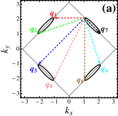
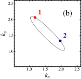
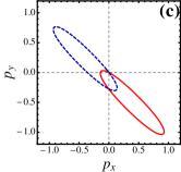
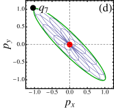
Figure 1: Illustration of the idea of the envelope model. Here for simplicity we choose $t^{\prime}=\mu=0$ and $\Delta_{0}=0.2t$. (a) CCE’s determined by $E_{\mathbf{k}}=|\omega|$ with $\omega=-0.4t$. The normal state Fermi surface is also shown. (b), CCE-1 in the first quadrant of FBZ. Two $\mathbf{k}$ points (red and blue dots) are shown. (c), two curves determined by $E_{\mathbf{k+p}}=|\omega|$ with red solid corresponds to $\mathbf{k}$ point 1 while blue dashed one to 2 in (b). (d), the envelope is shown in green solid line and central red dot. For schematic illustration we also draw in blue color a cluster of curves for several different $\mathbf{k}$’s. $\mathbf{q}_{7}$ as shown in (a) is located on the tip of the elliptic envelope.

In Fig. 1, we show the CCEs given by $E_{\mathbf{k}}=|\omega|$, which consists of 4 banana-shaped closed curves and are denoted as CCE-1,2,3,4 hereafter. To better elucidate our idea, we first focus on the intra-CCE contribution (i.e. both $\mathbf{k}$ and $\mathbf{k+p}$ on the same banana) to the JDOS. We examine the CCE in the first quarter of the FBZ, i.e. CCE-1. Corresponding to each $\mathbf{k}$ on CCE-1, all $\mathbf{p}$ points satisfying $E_{\mathbf{k+p}}=|\omega|$ form a closed curve denoted as $U_{\mathbf{k}}(\mathbf{p})$, which has exactly the same shape as CCE-1 except that the center is shifted as shown in Fig. 1(c). Therefore, for all $\mathbf{k}$’s on CCE-1, $U_{\mathbf{k}}(\mathbf{p})$’s form a one-parameter family of curves whose envelope is plotted in Fig. 1(d) shown as the green line and red dot. One can readily see that the envelope gives the locus on which the JDOS is most likely strong because it represents the position where curves in the family touch or intersect most.

Quantitative analysis can be obtained under the Dirac cone approximation. Accordingly CCE-1 is an ellipse whose semi-axis lengths are $a\equiv|\omega|/v_{\Delta}$ and $b\equiv|\omega|/v_{\text{F}}$. The corresponding family of curves $U_{\mathbf{k}}(\mathbf{p})$’s as shown in Fig. 1(d) are determined from the following equations, $(p_{1},p_{2})=(a\cos\theta-k_{1},b\sin\theta-k_{2})$ with $(k_{1},k_{2})=(a\cos\phi,b\sin\phi)$, where $\theta,\phi\in[0,2\pi)$. The envelope of the above family is composed of an ellipse and a trivial isolated point,

$$E_{\mathbf{p}}=2|\omega|,\ \ \ E_{\mathbf{p}}=0.$$ (14)

Taking advantage of the envelope functions, we can evaluate the JDOS’s divergence behavior just on these curves by integrating Eq. (13), which is relatively simpler than calculating $J(\mathbf{p},\omega)$ for arbitrary $\mathbf{p}$. We find that the relative amplitude of the inverse-square-root divergence is proportional to $\cos^{2}\theta$ on the elliptic envelope and the divergence is a $\delta$ function on the isolated point. As for the inter-CCE case between CCE-1 and CCE-3, the envelope consists of an ellipse and an isolated point similar to the intra-CCE case except that the center is shifted by a vector $\mathbf{n}_{3}-\mathbf{n}_{1}$ and the relative amplitude on the ellipse changes to $(1+\sin\theta)^{2}$. All these results are in a full agreement with former explicit formulas.

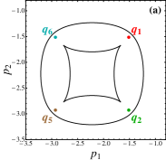
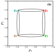
Figure 2: Plot of the envelope function according to Eq. (15), as well as 4 octet momenta $\mathbf{q}_{1,2,5,6}$. (a), less anisotropic case $\gamma=v_{\Delta}/v_{\text{F}}=0.4$ ($\Delta_{0}=0.4t$, $\omega=-0.8t$). (b) strong anisotropic case $\gamma=v_{\Delta}/v_{\text{F}}=0.1$ ($\Delta_{0}=0.1t$, $\omega=-0.2t$). Note that the anisotropy is determined by $\Delta_{0}/t$. We choose different $\omega$ just to have similar octet $q$’s for this two cases.

More importantly, the envelope analysis can be applied to the inter-CCE case between CCE-1 and CCE-2, which is otherwise rather complicated. The family of curves $U_{\mathbf{k}}(\mathbf{p})$’s satisfy, $(p_{1},p_{2})=-(k_{\text{F}},k_{\text{F}})+(b\cos\theta-k_{1},a\sin\theta-k_{2})$, where $k_{\text{F}}=\sqrt{2}\eta$ denotes the length of the Fermi vector at the nodes. The corresponding envelope is

$$\left\{\begin{array}[]{cc}p_{1}=-k_{\text{F}}+a\cos\alpha\left[\gamma^{2}s_{\gamma}(\alpha)\pm r_{\gamma}(\alpha)\right],\\ p_{2}=-k_{\text{F}}+a\sin\alpha\left[s_{\gamma}(\alpha)\pm\gamma^{2}r_{\gamma}(\alpha)\right],\end{array}\right.$$ (15)

where $r_{\gamma}(\alpha)=(\cos^{2}\alpha+\gamma^{2}\sin^{2}\alpha)^{-1/2}$ and $s_{\gamma}(\alpha)=(\sin^{2}\alpha+\gamma^{2}\cos^{2}\alpha)^{-1/2}$ with $\gamma\equiv b/a=v_{\Delta}/v_{\text{F}}$ is the anisotropic factor. This envelope is plotted in Fig. 2, where a circle-like [”$+$” sign in Eq. (15)] and an astroid-like curve [”$-$” sign in Eq. (15)] centered at $(-k_{\text{F}},-k_{\text{F}})$note is clearly seen. Also shown are the 4 wave vectors ($\mathbf{q}_{1,2,5,6}$ as in Fig. 1(a)) according to the octet model. One of our main findings is that, the anisotropy of the quasiparticle excitation spectrum plays a significant role in bridging the JDOS picture and the octet model. We find that the octet vectors $\mathbf{q}_{1,2,5,6}$ approach the cusps (most divergent as shown later) of the astroid for sufficient large anisotropy of the Dirac cone, while depart from the cusps of the astroid for the less anisotropic case, as shown in Fig. 2. This indicates that the effectiveness of the octet modelHoffman ; McElroy03nature ; qhwang is actually associated with the strong anisotropy of the quasiparticle excitations in $d$-wave cuprates.

On the circle-like and astroid-like envelopes, we again find the inverse square root divergence of JDOS similar to the intra-CCE case, with the relative amplitude (the coefficient of the divergent terms),

$$F_{\pm}(\alpha)\propto g_{\pm}(\alpha)\left[\left|\frac{s_{\gamma}(\alpha)}{r_{\gamma}(\alpha)}\pm\frac{r^{2}_{\gamma}(\alpha)}{s^{2}_{\gamma}(\alpha)}\right|^{-\frac{1}{2}}+(r\leftrightarrow s)\right],$$ (16)

with

$$g_{\pm}(\alpha)=[1\pm\gamma r_{\gamma}(\alpha)\sin\alpha][1+\gamma s_{\gamma}(\alpha)\cos\alpha].$$ (17)

According to Eq. (16), the amplitude $F_{-}(\alpha)$ on the astroid diverges when approaching its 4 cusps at $\alpha=\pi/4,3\pi/4,5\pi/4,7\pi/4$, coinciding with the octet vectors $\mathbf{q}_{1,2,5,6}$ in the large anisotropic case as shown in Fig. 2. This observation agrees well with the autocorrelation of the ARPES data McElroy . The effect of the coherence factors is embodied by $g_{\pm}(\alpha)$ in Eq. (16), inducing an additional angular dependence of the amplitudes. Accordingly the amplitudes on the astroid- and circle-like envelopes are highly uneven with one half is rather larger than the other half, breaking the four-fold symmetry possessed by the envelopes. Thus these two pronounced parts combine together to form a duck-foot structure as shown in Fig. 3. Note that in the same spirit, the relative amplitude of divergence of the ESS on these envelopes can also be obtained (not shown here as the quantitative numerical analyses of the ESS have been presented beforeqhwang ; scalapino ; franz ; csting ; Zhu ).

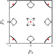
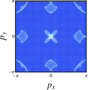
Figure 3: Comparison of analytical and numerical results of the JDOS in the first Brillouin zone. The parameters are $t^{\prime}=-0.3t$, $\mu=-1.0t$, $\Delta_{0}=0.2t$, $\omega=-0.2t$. Left: Plot of all the envelopes. The gray levels on the curves signal the relative amplitudes of divergence. Right: Numerical results according to Eq. (13) with lattice size $400\times 400$, where $\delta(x)\approx\frac{\eta_{0}}{\pi(x^{2}+\eta_{0}^{2})}$ with $\eta_{0}=0.01t$.

Combining the above analyses, we can plot all the envelopes where $J(\mathbf{p},\omega)$ diverges in Fig. 3(a) with the relative amplitude of divergence being taken into consideration. We find two cigars centered at the origin, four duck feet on the coordinate axes and four (semi)cigars on the zone corners as well as five red dots. The envelope analysis capture the essential structures and symmetries of the JDOS, in excellent agreement with the experimental data McElroy as well as the JDOS by numerical integration of Eq. (13) as shown in Fig. 3(b). As for the peak positions, $\mathbf{q}_{7}$ and $\mathbf{q}_{4}$ locate on vertices of the central and corner cigars respectively. $\mathbf{q}_{1,2,5,6}$ is on apexes of the duck feet. $\mathbf{q}_{3}$ lies on the center of the corner cigars denoted as red dot. All these features are in full consistent with the experimental observations McElroy .

In summary, the JDOS and ESS in $d$-wave superconductors have been investigated analytically, both being found to diverge on the curves of envelopes. Using the envelope scenario by us, we have shown clearly that the the octet vectors locate on the vertices of the envelopes validating the octet model for the $d$-wave cuprates with strong anisotropy of the quasiparticle excitation spectrum. The relative amplitude of the divergence of the JDOS has been obtained. Finally, we wish to pinpoint that the envelope scenario may also be used to investigate the JDOS of the iron-based superconductors, which may shed light on the Fermiology and pairing symmetry in this new material.

The work was supported by the RGC of Hong Kong under Grant No.HKU7055/09P and HKUST3/CRF/09, the URC fund of HKU, the Natural Science Foundation of China No.10674179.

References

- (1) Ø. Fischer, M. Kugler, I. Maggio-Aprile, C. Berthod and C. Renner, Rev. Mod. Phys. 79, 353 (2007).
- (2) J. E. Hoffman, K. McElroy, D.-H. Lee, K. M. Lang, H. Eisaki, S. Uchida and J. C. Davis, Science 297, 1148 (2002).
- (3) K. McElroy, R. W. Simmonds, J. E. Hoffman, D.-H. Lee, J. Orenstein, H. Eisaki, S. Uchida and J. C. Davis, Nature (London) 422, 592 (2003).
- (4) Q.-H. Wang and D.-H. Lee, Phys. Rev. B 67, 020511 (2003).
- (5) L. Capriotti, D. J. Scalapino and R. D. Sedgewick, Phys. Rev. B 68, 014508 (2003).
- (6) T. Pereg-Barnea and M. Franz, Phys. Rev. B 68, 180506(R) (2003).
- (7) D.-G. Zhang and C. S. Ting, Phys. Rev. B 69, 012501 (2004).
- (8) L. Zhu, W. A. Atkinson and P. J. Hirschfeld, Phys. Rev. B 69 060503(R) (2004).
- (9) K. McElroy, G.-H. Gweon, S. Y. Zhou, J. Graf, S. Uchida, H. Eisaki, H. Takagi, T. Sasagawa, D.-H. Lee and A. Lanzara, Phys. Rev. Lett. 96, 067005 (2006).
- (10) In the local coordinate system the center of the astroid- and circle-like envelopes locates at . More generally, it is .