VLA Observations of the Infrared Dark Cloud G19.30+0.07

Abstract

We present Very Large Array observations of ammonia (NH₃) (1,1), (2,2), and CCS ($2_{1}-1_{0}$) emission toward the Infrared Dark Cloud (IRDC) G19.30+0.07 at $\sim 22$ GHz. The NH₃ emission closely follows the 8 $\mu$m extinction. The NH₃ (1,1) and (2,2) lines provide diagnostics of the temperature and density structure within the IRDC, with typical rotation temperatures of $\sim 10$ to 20 K and NH₃ column densities of $\sim 10^{15}$ cm^-2. The estimated total mass of G19.30+0.07 is $\sim$1130 M_☉. The cloud comprises four compact NH₃ clumps of mass $\sim 30$ to 160 M_☉. Two coincide with 24 $\mu$m emission, indicating heating by protostars, and show evidence of outflow in the NH₃ emission. We report a water maser associated with a third clump; the fourth clump is apparently starless. A non-detection of 8.4 GHz emission suggests that the IRDC contains no bright H ii regions, and places a limit on the spectral type of an embedded ZAMS star to early-B or later. From the NH₃ emission we find G19.30+0.07 is composed of three distinct velocity components, or “subclouds.” One velocity component contains the two 24 $\mu$m sources and the starless clump, another contains the clump with the water maser, while the third velocity component is diffuse, with no significant high-density peaks. The spatial distribution of NH₃ and CCS emission from G19.30+0.07 is highly anti-correlated, with the NH₃ predominantly in the high-density clumps, and the CCS tracing lower-density envelopes around those clumps. This spatial distribution is consistent with theories of evolution for chemically young low-mass cores, in which CCS has not yet been processed to other species and/or depleted in high-density regions.

1 Introduction

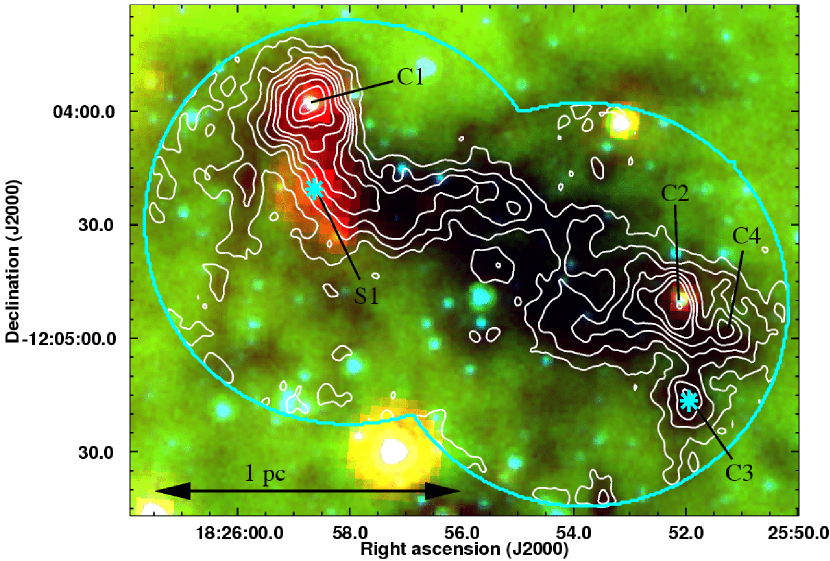
Figure 1: 4.5 $\mu$m (blue), 8.0 $\mu$m (green), and 24 $\mu$m (red) 3-color image of IRDC G19.30+0.07. White contours represent the integrated intensity from the main hyperfine component of the NH₃ (1,1) line. The NH₃ (1,1) resolution is $4\farcs 5\times 3\farcs 4$ and RMS noise at the center of the primary beam is $\sim 5$ mJy beam^-1 km s^-1. Contours mark 4$\sigma$, 8$\sigma$, 12$\sigma$, 16$\sigma$, and 20$\sigma$ and then increase in 8$\sigma$ intervals, where $\sigma$ is defined at the center of the primary beam. Blue lines mark the 50% power point of the primary beam; noise levels at the edge of the field are twice those at the center of the primary beam. The light blue asterisks indicate H₂O maser detections (Wang et al., 2006, this paper). The four NH₃ clumps identified by this work are labeled C1, C2, C3, and C4.

Infrared dark clouds (IRDCs) are dense, cold molecular clouds seen in silhouette against 8 $\mu$m Galactic plane PAH emission. Dust is relatively transparent to 8 $\mu$m emission, so only the densest parts of molecular clouds (A_V $\gtrsim 50$) are opaque at this wavelength (Indebetouw et al., 2005). Since massive stars and their associated clusters form in massive and dense concentrations of dust and gas, it follows that the initial conditions of massive star formation are probably found in the highest density regions of molecular clouds. The GLIMPSE team imaged about two-thirds of the inner Galactic plane $|l|=0^{\circ}-65^{\circ}$ using the Spitzer Space Telescope (SST) Infrared Array Camera (IRAC) at 3.6, 4.5, 5.8, and 8 $\mu$m with better than $2\arcsec$ resolution (Benjamin et al., 2003). The GLIMPSE images contain thousands of IRDCs (Peretto & Fuller, 2009) with structure on size scales $\gtrsim 0.5\arcmin$ to as small as the IRAC resolution (see Figure 1). Because they are prominent in silhouette, IRDCs are generally expected to lie at the near kinematic distance. Preliminary studies show that IRDCs are cold ($\lesssim 20$ K) and dense ($n_{\rm H_{2}}\gtrsim 10^{5}$ cm^-3), and many have masses $\gtrsim 10^{3}$ M_☉ (Carey et al., 1998; Egan et al., 1998; Pillai et al., 2006; Redman et al., 2003; Rathborne et al., 2006, 2007; Wang et al., 2008). Pillai et al. (2007) detected high deuteration in IRDC clumps, evidence of very low temperatures. However, the details of the kinematics, chemistry, and star formation within IRDCs are not well understood. High resolution observations of IRDCs are needed to provide information on scales small enough to differentiate between cloud properties in quiescent and star forming regions, a distinction crucial to refining models of the earliest stages of massive star formation (Wang et al., 2008; Rathborne et al., 2006).

Here we report results of a detailed study of an IRDC at radio wavelengths using the Very Large Array (VLA) of the National Radio Astronomy Observatory. IRDC G19.30+0.07 ($\alpha$(J2000)=18^h25^m56^s, $\delta$(J2000)=$-$12^∘04′30″, V${}_{LSR}\sim 26$ km s^-1) is a filamentary IRDC with a length of $\sim 2$′ and a width of $\sim 30$″. Using a flat Galactic rotation curve with R${}_{0}=8.5$ kpc and V${}_{0}=220$ km s^-1, the kinematic distance to G19.30+0.07 is $\sim 2.4$ kpc. We have determined the physical and chemical properties of G19.30+0.07 using ammonia (NH₃) (1,1), (2,2), and dicarbon sulfide (CCS) ($2_{1}-1_{0}$) transitions (upper level energies ($E_{u}/k$) of 23.8 K, 65.0 K, and 1.6 K respectively) with an angular resolution roughly a factor of seven higher than previously reported for this IRDC, 6″ compared to $\sim 40$″ (Pillai et al., 2006; Sakai et al., 2008). To relate the gas properties to star formation, continuum observations at 8.4 GHz have been carried out to search for ionized gas associated with H ii regions in the IRDC.

NH₃ and CCS are important molecules for investigating IRDCs: both are typically considered to be high-density tracers ($n_{\rm H_{2}}\gtrsim 10^{4-6}$ cm^-3), and the relative strengths of NH₃ inversion lines can be used to estimate the temperature and column density of the gas (Ho & Townes, 1983). Furthermore, [CCS]/[NH₃] relative abundances may provide information about chemical evolution (Suzuki et al., 1992; van Dishoeck & Blake, 1998). Chemical models have mainly been developed from observations of low mass star forming regions; this study examines whether such models might also apply in IRDCs near young star forming clumps.

The main goal of this paper is to examine the physical and chemical properties of the IRDC G19.30+0.07 and explore the relationship between these properties and signs of star formation. The high spatial and spectral resolution of this study permits us to distinguish between multiple velocity components in the IRDC, map the temperature and density distributions in the IRDC at 6″ resolution, and examine the relative distribution of two gas species in the IRDC. This is one of the first IRDC studies to explore the role of multiple cloud components, distinguished by small offsets in velocity, within an IRDC. Furthermore, evidence for star formation and outflows in G19.30+0.07 enables us to examine the relationship between IRDC properties and star formation.

This paper is structured as follows: in §2, we present details of our VLA observations and data reduction. In §3, we present results of the NH₃, CCS, and continuum observations. In §4 we examine the gas kinematics and present the derived temperature, density, and mass distributions, as well as relative abundances of NH₃ and CCS in the IRDC. In §5 we discuss the relationship between physical and chemical properties, kinematics, and star formation within the IRDC. Conclusions are given in §6.

2 Observations and Calibration

Table 1 summarizes the parameters of the VLA observations. NH₃ (1,1) and (2,2) and CCS ($2_{1}-1_{0}$) emission at $\sim 22$ GHz were observed with the VLA in D configuration. The 3.125 MHz bandwidth contained the main and innermost satellite hyperfine lines of the NH₃ (1,1) and (2,2) transitions. Two pointings were used to fully cover the highest opacity regions, as determined from the 8 $\mu$m images. All data were calibrated and imaged using AIPS. The CCS observations were conducted during the EVLA upgrade, and eight of the twenty-seven antennas had been converted to EVLA antennas. Data were obtained using both the VLA and EVLA antennas. Doppler tracking could not be used during the upgrade period, so the AIPS task CVEL was applied during calibration to correct for motion of the Earth relative to the local standard of rest during the observations. In the 22 GHz datasets, the uncertainty of the absolute flux densities is estimated to be 10%. We estimate the absolute positional accuracy to be better than 1″.

Images were made of the two pointings at each frequency using natural weighting of the u-v data and CLEAN deconvolution. The AIPS task FLATN was used to mosaic the two pointings and apply a primary beam correction. The NH₃ (1,1) and (2,2) mosaics were cut off at the 50% power level of the primary beam. The synthesized beam in the full-resolution NH₃ images is $\sim 4$″; however, the NH₃ data were later smoothed to 6″ resolution to increase the signal-to-noise ratio prior to fitting the emission lines with Gaussian profiles as a function of velocity (see §4). The multiplication factors needed to convert from Jy beam^-1 to beam-averaged brightness temperature (K) for the various images are listed in Table 1.

Because the CCS emission is weak and extended relative to that of NH₃, a 30 k$\lambda$ Gaussian u-v taper was applied while imaging the data, resulting in a resolution of $7\farcs 7\times 5\farcs 7$. The u-v taper was chosen to maintain the highest resolution possible while still providing a significant ($\geq 3\sigma$) CCS detection. Additionally, a more conservative primary beam cutoff at the 65% power point was used while mosaicing the CCS so that noise peaks at the edges of the primary beam were not amplified into apparently significant detections at the low contour levels. The 65% power point cutoff was determined by reducing the primary beam cutoff until spurious $3\sigma$ detections no longer appeared at the image edges.

Continuum emission at 8.4 GHz was observed with the VLA in A configuration. These data were also calibrated and imaged with the AIPS reduction package, using the model for the flux calibrator supplied with the package. The uncertainty of the absolute flux density scale is estimated to be 10%. Robust u-v weighting and CLEAN deconvolution were used during imaging. The resolution of the resulting image is $\sim 0\farcs 3$.

We have also re-reduced and analyzed the G19.30+0.07 VLA H₂O maser data published by Wang et al. (2006) (project AW659; the full details of these observations are described by Wang et al.). The data for the two pointings toward G19.30+0.07 were reduced in the usual manner using AIPS. After self-calibration, the RMS noise in a single 0.66 km s^-1 wide channel is 20 mJy beam^-1 toward the NE pointing and 15 mJy beam^-1 toward the SW pointing. These noise levels are about five times better than those reported for the ensemble of sources observed by Wang et al. (2006). The synthesized beam for these maser data is approximately $1\farcs 5\times 0\farcs 9$.

3 Results

3.1 NH₃

The NH₃ (1,1) main line emission, integrated over 24.1 to 30.3 km s^-1, is shown overlaid on an infrared 3-color Spitzer image of G19.30+0.07 in Fig. 1. The three colors in Fig. 1 are GLIMPSE 4.5 $\mu$m (blue) and 8 $\mu$m (green) emission and MIPSGAL (Carey et al., 2009) 24 $\mu$m emission (red). Fig. 1 shows that the NH₃ (1,1) emission is spatially well correlated with the 8 $\mu$m extinction. NH₃ (2,2) emission was also detected throughout the IRDC, although due to the fainter line emission the (2,2) emission was not as well defined near the IRDC boundaries. The RMS noise in the NH₃ (1,1) integrated intensity image is 5 mJy beam^-1 km s^-1.

In our discussions of IRDC structure, we use the guidelines described by Bergin & Tafalla (2007): clouds have masses of $\sim 10^{3}$ to 10⁴ M_☉ and radii of $\sim 1$ to 10 pc, clumps have masses of $\sim 10^{2}$ to 10³ M_☉ and radii of $\sim 0.1$ to 1 pc, and cores have masses of $\sim 1$ to 10² M_☉ and radii of $\sim 0.01$ to 0.1 pc. Clumps produce star clusters, and cores produce individual stars. A 20″ FWHM Gaussian unsharp mask was used to identify the compact structure in G19.30+0.07. The selection criteria for NH₃ clumps were peaks having structure $\lesssim 20\arcsec$ with integrated intensities $\gtrsim 25$ Jy beam^-1 km s^-1 in the masked image. G19.30+0.07 contains four apparent NH₃ clumps, labeled in Fig. 1 as C1, C2, C3, and C4. C1 and C2 coincide with 24 $\mu$m emission and have previously been studied at mm wavelengths with $\sim 11\arcsec$ resolution (Rathborne et al., 2006). C3 is not associated with any 24 $\mu$m emission; however, a H₂O maser is located nearby (see §3.4). C4 is an NH₃ emission peak not associated with any IR emission or masers. The 24 $\mu$m source S1 (Fig. 1) is not coincident with a peak in the NH₃ emission. There is a H₂O maser with velocity 19 km s^-1 (Wang et al., 2006) spatially coincident with S1. This maser’s velocity is slightly offset from the velocity of G19.30+0.07, $\sim 26$ km s^-1. While it is possible that the maser is associated with an unrelated object along the line of sight, the probability of two dense cores capable of forming a H₂O maser along the line of sight to S1 is small. It is more probable that the velocity offset between the maser and the IRDC is caused by motion within the IRDC related to star formation activity (Wang et al., 2006).

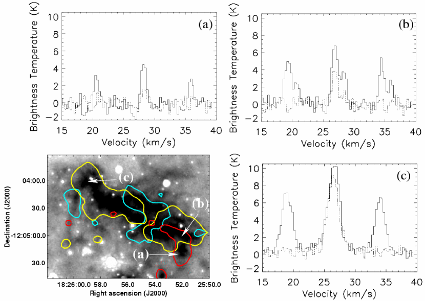
Figure 2: Three representative line profiles of NH₃ (1,1) and (2,2) emission from three different positions in G19.30+0.07. The solid and dot-dashed lines show the (1,1) and (2,2) data, respectively. Profile (a) shows a single velocity line profile, observed at $\alpha$(J2000)=18^h25^m52.2^s, $\delta$(J2000)=$-$12^∘05′20$\farcs$7. Profile (b) shows emission from multiple velocity components, separated by $\sim 1.5$ km s^-1, observed at $\alpha$(J2000)=18^h25^m52.1^s, $\delta$(J2000)=$-$12^∘04′59$\farcs$9. Profile (c) is from a point in the northern ammonia clump, $\alpha$(J2000)=18^h25^m58.8^s, $\delta$(J2000)=$-$12^∘04′02$\farcs$9, showing a broad line-wing component. The locations of the representative profiles are indicated on the GLIMPSE 8 $\mu$m image. The line profiles were used to identify three subclouds, separated by velocity offsets $\sim 1$ km s^-1. The subcloud locations are shown overlaid on the GLIMPSE 8 $\mu$m image; the subcloud velocities are centered at 28.4 km s^-1 (red), 26.7 km s^-1 (yellow), and 25.7 km s^-1 (blue).

Multiple velocity components and broad line-wing structures are evident in the NH₃ emission, as shown in Figure 2. Double-line profiles indicate locations in the cloud where there are two overlapping kinematic components. The double-line profile features cannot be attributed to self-absorption: as demonstrated in Fig. 2b, the double-line profile structure is seen in the more optically thin (2,2) emission as well as the (1,1) emission. Furthermore, the double-line profiles are not correlated with NH₃ high optical depth (see §4.2). Finally, the individual components of the double-line profiles can be traced continuously from regions with single-line profiles at the same velocity; it is in overlap regions that they appear double, as illustrated by the profiles shown in Fig. 2. There are three distinct velocity components over the entire G19.30+0.07 dark cloud, which we will henceforth refer to as “subclouds.” The spatial extents of these subclouds are derived from fits to the NH₃ line profiles, as described in §4.1. The subcloud positions relative to the 8 $\mu$m emission are shown in Fig. 2.

3.2 CCS

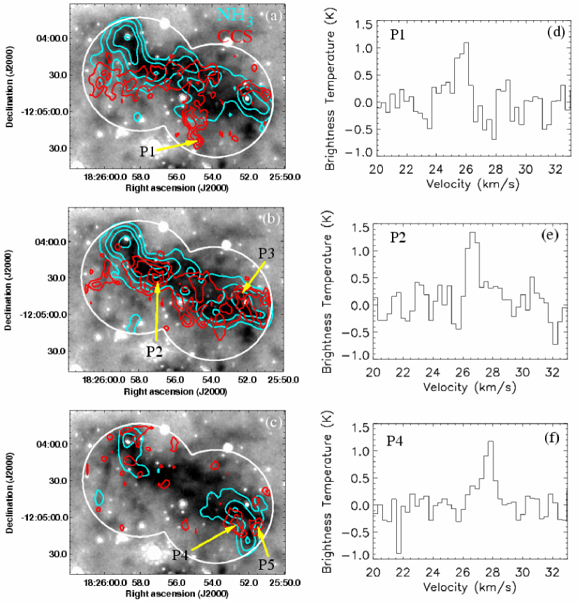
Figure 3: CCS ($2_{1}-1_{0}$) distribution in IRDC G19.30+0.07 and representative profiles of CCS emission. The greyscale is the 8.0 $\mu$m image from GLIMPSE. Red contours represent CCS ($2_{1}-1_{0}$) emission integrated over different velocity components: (a) 25.2 to 26.5 km s^-1, (b) 26.2 to 27.4 km s^-1, and (c) 27.7 to 28.9 km s^-1. The angular resolution of the CCS image is $7\farcs 7\times 5\farcs 7$. The CCS RMS noise is 1.3 mJy beam^-1 km s^-1. CCS increments start at 3$\sigma$ and increase in 2$\sigma$ increments, where $\sigma$ is defined at the center of the primary beam. The white contours show where the detection power of the primary beam in the CCS observations drops to 65%. Blue contours represent NH₃ (1,1) emission smoothed to match the CCS resolution (7$\farcs$7$\times$5$\farcs$7) and averaged over the same velocity ranges. The NH₃ RMS noise is 1.8 mJy beam^-1 km s^-1, and the contours indicate emission levels of 10$\sigma$, 30$\sigma$, 60$\sigma$, and 100$\sigma$. Arrows indicate CCS peaks, labeled P1, P2, P3, P4, and P5. Representative profiles toward P1, P2, and P4 are shown in (d), (e), and (f), respectively.

Where both CCS and NH₃ emission is detected their velocities match very well. However, in many locations there is emission from one molecule and not the other. Figure 3 shows the distribution of the CCS and the NH₃ (1,1) main line emission along with representative CCS profiles; peaks in the CCS emission have been labeled as P1-P5. The CCS in Fig. 3 is integrated over four channels (1.2 km s^-1) centered on the velocities of the subclouds as determined from the NH₃ emission. The NH₃ emission in Figure 3 has been smoothed to match the resolution of the CCS emission ($7\farcs 7\times 5\farcs 7$) and integrated over the same velocity ranges. The RMS noise in the CCS integrated intensity images is 1.3 mJy beam^-1 km s^-1.

3.3 8.4 GHz Continuum

No 8.4 GHz continuum emission is detected from G19.30+0.07. The RMS noise in the field is 0.025 mJy beam^-1. A 5$\sigma$ (0.125 mJy) upper limit on any free-free continuum emission implies an upper limit on the UV photon flux of $N_{c}\lesssim 8\times 10^{43}$ s^-1 (Mezger & Henderson, 1967; Condon, 1992). However, it is unlikely that all of the emitted UV photons go into ionization of H and He. The UV flux could be reduced by absorption by an accretion disk or dust surrounding the protostar. Thus, the UV flux limit is likely an underestimate of $N_{c}$. Furthermore, early-stage H ii regions can be small, dense, and optically thick, and consequently have low radio continuum flux densities. Further discussion of the protostellar mass limit implied by the UV flux limit is given in §5.3.

3.4 H₂O Masers

From our re-reduction and analysis of the Wang et al. (2006) H₂O maser data we have detected two regions of maser emission. A previously unreported maser with a peak flux density of 1.58 Jy was detected at $\alpha$(J2000)=18^h25^m51.95^s, $\delta$(J2000)=$-$12^∘05′14$\farcs$0 at an LSR velocity of 28.8 km s^-1. This maser is located within the C3 ammonia clump (Fig. 1), and is the first reported evidence of star formation associated with this clump. The second H₂O maser, first reported in Wang et al. (2006), has a peak flux density and velocity of 0.51 Jy and 19.0 km s^-1, respectively, at a position of $\alpha$(J2000)=18^h25^m58.64^s, $\delta$(J2000)=$-$12^∘04′21$\farcs$5. This maser is located close to the 24 $\mu$m source S1. The reported peak flux densities have been corrected for primary beam attenuation.

4 Physical Properties of the Dense Gas

4.1 Gas Kinematics

The line profiles from the spatially smoothed $6\arcsec\times 6\arcsec$ resolution NH₃ (1,1) and (2,2) images have been fitted using a non-linear least squares Gaussian fitting routine, providing central velocities, linewidths, and amplitudes. Fitting errors for the NH₃ central velocity and linewidths are typically $\lesssim 0.1$ km s^-1, and $\lesssim 10$% for the amplitude, with the uncertainty reduced by approximately a factor of two in areas with a high signal-to-noise ratio.

The (1,1) line fitting was done in two steps. First, the main (1,1) line was fitted. Second, the main line and two satellite hyperfine lines were fit simultaneously with a triple-gaussian profile, using the results from the first (main-line only) fit to set initial guesses for, and constraints on, the fits to the satellite lines. The initial guesses and constraints were set as follows: (1) the initial guesses for the central velocities of the satellite lines were set at the velocity of the main line $\pm 7.7$ km s^-1, constrained to $\pm 0.6$ km/s of this initial guess; (2) the initial guess for the width of the satellite lines was set to the width of the main line, constrained to $\pm 0.6$ km s^-1. The fit to the (2,2) line was not constrained by the results of the (1,1) fit.

In areas with double-line profiles (see Fig. 2), the fitting included additional steps. One of the (1,1) main lines and its associated satellite lines were fitted as described above. Then the second (1,1) main and satellite lines were fitted as described above. Finally, the results of these fits were used to set the initial guesses and constraints for a simultaneous (six-gaussian) fit that separated the various emission contributions. The double-profile fits of the satellite lines used the same main-line based constraints as described for single-profile fits. The fits to (2,2) double-line profiles were done simultaneously using a two-gaussian profile; as in the single-profile case, the fits were not constrained by the (1,1) line fits. C1 and C2 exhibit an emission component with broad line-wings, possibly indicating outflows; in these areas the line-wing component was modeled as an additional Gaussian during simultaneous line fitting.

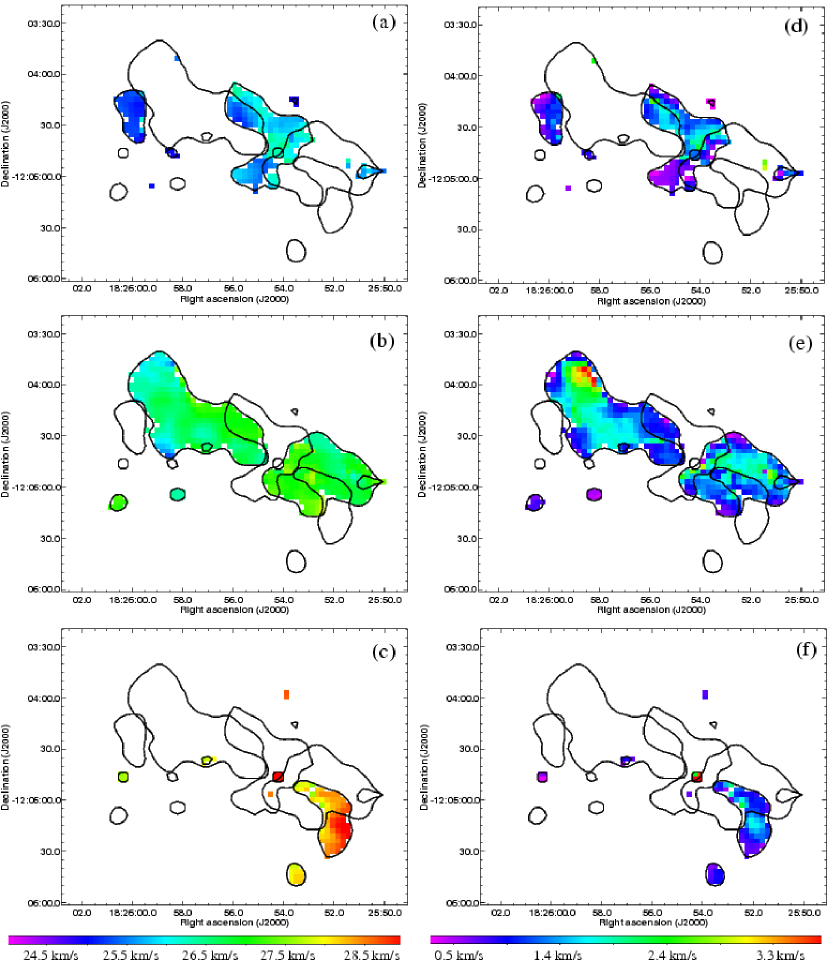
Figure 4: Velocities and FWHM linewidths within the three subclouds that make up G19.30+0.07. Pixel spacing is 3″, resolution is 6″. Black outlines indicate the boundaries of the different subclouds identified in Fig. 2. The LSR velocities are shown in (a), (b) and (c), and the NH₃ (1,1,$m$) FWHM linewidths are shown in (d), (e), and (f). Velocity components are centered at 25.7 km s^-1 in (a) and (d), 26.7 km s^-1 in (b) and (e), and 28.4 km s^-1 in (c) and (f).

Three subclouds were identified based on fits of the NH₃ (1,1) profiles. Their median LSR velocities are centered at 25.7 km s^-1, 26.7 km s^-1, and 28.4 km s^-1. The spatial distributions of the velocities and linewidths for each of the subclouds are shown in Figure 4. Internal motion is indicated within each subcloud by central velocity changes of $\lesssim 1$ km s^-1, shown in Figs. 4a, 4b, and 4c. Typical FWHM linewidths are $\sim 1.2$ km s^-1, but the linewidths are $\sim 0.6$ km s^-1 at the subcloud boundaries and increase to $\gtrsim 2$ km s^-1 near C1 and C4, shown in Figs. 4d, 4e, and 4f. Since C4 contains no evidence of star formation, the increased velocity dispersion at C4 may be due to a nearby outflow originating from C2.

As discussed in §3.2, CCS emission is found in all of the subclouds. The CCS emission lines could not be fitted reliably because of their low signal-to-noise ratio, but based on the profiles shown in Fig. 3 we estimate the CCS FWHM to be $\sim 0.6$ km s^-1, and therefore assume the CCS emission from each subcloud is contained within $\sim 1.2$ km s^-1 centered at that subcloud’s velocity. Where both CCS and NH₃ are detected, the linewidths and emission line structure from both molecules are in good agreement, even in areas with multiple velocity components. Thus, CCS velocity components were separated by averaging over 1.2 km s^-1 centered at the subcloud velocities determined from NH₃.

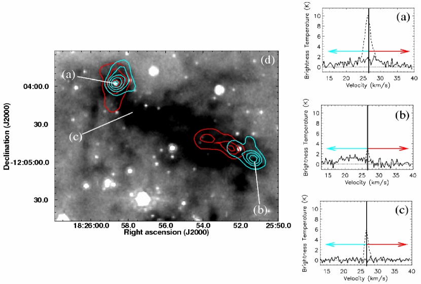
Figure 5: Broad line-wings in addition to narrow NH₃ emission are found near C1 and C2. Three representative profiles of the NH₃ (2,2) emission are shown from different locations in G19.30+0.07. In (a), (b), and (c), the total (2,2) line emission is shown as a dashed line and the residual emission (line-subtracted, as described in the text) is shown as a solid line. In (a) and (b), broad line-wing components are present; for comparison, (c) lacks line-wing emission. The locations of the representative profiles are indicated on the GLIMPSE 8 $\mu$m image (d). Contours in (d) show integrated intensity from the NH₃ (2,2) residual images. The blue and red-shifted line-wing emission was integrated over 14.6 to 26.6 km s^-1 and 26.6 to 38.7 km s^-1; these velocity ranges are indicated by red and blue arrows in (a), (b), and (c). Blue contours represent the integrated intensity blue-ward of the NH₃ (2,2) line center, and red contours represent the integrated intensity red-ward of the NH₃ (2,2) line center. The 1$\sigma$ uncertainty in the emission integrated over 6 km s^-1 is $\sim 0.025$ Jy beam^-1 km s^-1. Contours show 2$\sigma$, 6$\sigma$, and then increase in 3$\sigma$ intervals.

NH₃ (2,2) line profiles were used to examine the kinematics of the line-wing features, as the greater separation between the main line and satellite hyperfine components for the (2,2) transition simplified simultaneous fitting of narrow and broad components. The line-wings toward C1 and C2 had typical FWHM linewidths of $\sim 12$ km s^-1. A residual image cube was made of the NH₃ emission with the fitted narrow component subtracted, so that only the broad component remained. The integrated blue- and red-shifted emission was obtained from the residual data by integrating over the velocity ranges 14.6 to 26.6 km s^-1 and 26.6 to 38.7 km s^-1. Representative profiles and the red- and blue-shifted integrated NH₃ (2,2) emission are shown in Figure 5.

The red and blue line-wing emission from C1 is spatially coincident with, and centered on, a 24 $\mu$m source, and can be interpreted as an outflow oriented close to the line of sight. The infall velocity derived from the mass and radius of C1 (see §4.4) is $\sim 2$ km s^-1, insufficient to account for the broadening observed in the line-wing emission. The age of C1’s outflow cannot be determined from the flow velocities because of the line-of-sight orientation. The line-wing emission at C2 can be interpreted as an outflow originating at the 24 $\mu$m source, with the red shifted outflow extending $\sim 0.4$ pc NE and the blue shifted outflow extending $\sim 0.3$ pc SW of the source. The outflow from C2 appears well collimated, with a collimation factor (length/width) $\gtrsim 5$. The outflow’s inclination angle is unknown, so we assume an angle of 45^∘ in estimating the measured length of the outflow. The central velocity derived from a Gaussian fit to the broad component at each pixel within the C2 outflow gives an average outflow velocity of $\sim 5$ km s^-1, corrected for an assumed inclination angle of 45^∘. The outflow’s kinematic age was determined by dividing the extent of the outflow by the average outflow velocity, resulting in an age of $\sim 10^{5}$ yr.

4.2 Optical Depth, Temperature, and Density Structure

NH₃ inversion transitions have hyperfine splitting due to magnetic dipole interactions and the interaction of the nitrogen electric quadrupole moment and the electron electric field (Ho & Townes, 1983). The optical depth of the NH₃ (1,1) main line, $\tau_{(1,1,m)}$, can be derived from the ratio of the main and satellite hyperfine line strengths. Assuming the excitation temperature is the same for the main and satellite lines, the ratio of the brightness temperatures $T_{b(1,1,m)}$ and $T_{b(1,1,s)}$ can be expressed as

$$\frac{T_{b(1,1,m)}}{T_{b(1,1,s)}}=\frac{1-\exp[-\tau_{(1,1,m)}]}{1-\exp[-\alpha\tau_{(1,1,m)}]}$$ (1)

where ‘$m$’ and ‘$s$’ indicate the main and satellite hyperfine components, $T_{b}$ is the measured brightness temperature, $\tau_{(1,1,m)}$ is the optical depth of the main quadrupole hyperfine component of the (1,1) line, and $\alpha$ is the theoretical intensity ratio of the satellite line to the main line if the hyperfine levels are populated according to their statistical weights. For the innermost satellite hyperfine transition, $\alpha=0.28$ (Rydbeck et al., 1977).

The total optical depth of the (1,1) line, $\tau_{(1,1)}$, can be determined from $\tau_{(1,1,m)}$ and the relative intensities of the hyperfine components, such that $\tau_{(1,1)}=\zeta\tau_{(1,1,m)}$, where $\zeta$ is the ratio of the total (1,1) line optical depth to the optical depth of the main hyperfine component. If the NH₃ (1,1) hyperfine levels are populated according to their statistical weights, $\zeta=2$ (Rydbeck et al., 1977).

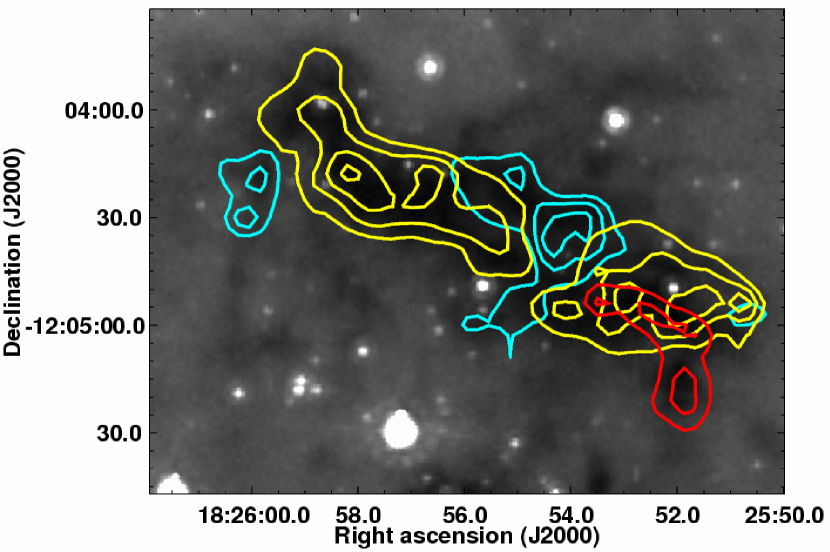
Figure 6: The optical depth of NH₃ (1,1) in the three subclouds is shown. The components are centered at 28.4 km s^-1 (red), 26.7 km s^-1 (yellow), and 25.7 km s^-1 (blue). Contours start at $\tau$(1,1)=3 and increment by 3.

The optical depth $\tau_{(1,1)}$ ranges from $\sim 1$ to 4 at the boundaries of the subclouds and increases towards the cloud centers. Near C1, C2, and C3 $\tau_{(1,1)}$ is $\sim 5$ to 10. The uncertainty in $\tau_{(1,1)}$ is $\lesssim 30$% where the NH₃ signal to noise is highest. At the subcloud boundaries, the uncertainty in $\tau_{(1,1)}$ increases, and is on the order of a factor of two. At positions where $\tau_{(1,1)}>20$, $T_{b(1,1,s)}$ approaches $T_{b(1,1,m)}$ too closely to yield accurate results; at these positions a $\tau_{(1,1)}$ value of 20 was assumed. The optical depth distribution is shown in Figure 6. It is notable that areas where NH₃ double-line profiles are detected, shown as subcloud overlap in Fig. 2, are not coincident with the highest optical depth gas, ruling out self-absorption as a cause of the double peaked line profile.

The ratio of the brightness temperatures of the NH₃ (1,1,$m$) and (2,2,$m$) lines can be used to determine the rotation temperature $T_{R}(1,1:2,2)$ that characterizes the population distribution among the (1,1) and (2,2) states (Ho & Townes, 1983):

$$T_{R}(1,1:2,2)=-41.5\left(\ln{\biggl{[}-\frac{0.284}{\tau_{(1,1,m)}}\ln{\Bigl{[}1-\frac{T_{b(2,2,m)}}{T_{b(1,1,m)}}\bigl{(}1-\exp[-\tau_{(1,1,m)}]\bigr{)}\Bigr{]}}\biggr{]}}\right)^{-1}.$$ (2)

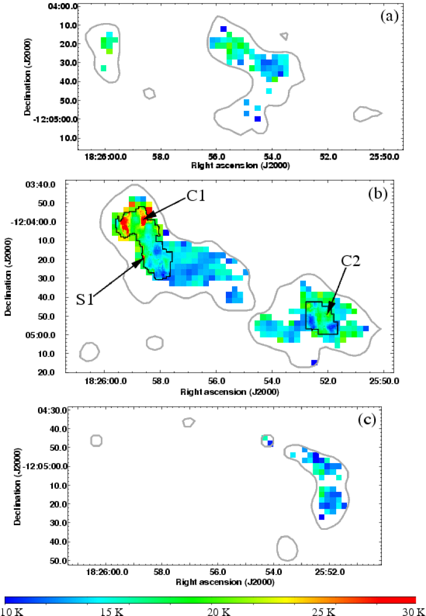
Figure 7: The NH₃ rotation temperature distribution in the three subclouds is shown. Only points with uncertainty $\leq 10$% have been mapped. Grey outlines indicate the boundaries of the different subclouds. The component centered at 25.7 km s^-1 is shown in (a), 26.7 km s^-1 in (b), and 28.4 km s^-1 in (c). The resolution in the images is 6″ except in the areas outlined in black in (b), which have a higher resolution of $4\farcs 5\times 3\farcs 4$ and pixel spacing 0$\farcs$5. Arrows in (b) indicate the locations of C1, C2, and S1.

The distribution of $T_{R}$ for locations where the statistical uncertainty in $T_{R}$ is 10% or less is shown in Figure 7. The $T_{R}$ gradient is steep near the NH₃ clumps, and consequently $T_{R}$, in particular, suffers from the effects of beam dilution caused by smoothing the data. Thus, we created temperature maps at the original $\sim 4$″ resolution of C1 and C2, where the NH₃ emission is strong enough to obtain good line fits. The higher resolution images are shown outlined in black in Fig. 7(a).

Values of $T_{R}$ range from 10 K up to $\sim 30$ K, above which $T_{b(2,2,m)}$ approaches $T_{b(1,1,m)}$ too closely to yield reliable temperature estimates. A value of 35 K was assumed at points where $T_{b(2,2,m)}\sim T_{b(1,1,m)}$ to indicate points with uncertain temperatures. The higher resolution images of the clumps show that $T_{R}$ reaches this maximum at C1 and S1, and $T_{R}\sim 20$ K in C2, indicating heat sources at these locations. Heating is consistent with the presence of 24 $\mu$m emission in C1, C2, and S1. An area with $T_{R}\geq 35$ K approximately 10″ east of C1 has no corresponding peak in NH₃, and the nature of this peak in $T_{R}$ remains unknown.

Using earlier results from Danby et al. (1988), Tafalla et al. (2004) empirically find a relationship between IRDC gas kinetic temperature, $T_{K}$, and $T_{R}$,

$$T_{K}\approx\frac{T_{R}}{1-\frac{T_{R}}{42}{\rm ln}\Bigl{[}1+1.1{\rm exp}(\frac{-16}{T_{R}})\Bigr{]}}.$$ (3)

This relationship is good to better than 5% when $T_{R}$ is 5 to 20 K. Above 20 K, the relationship is not as accurate. Since the majority of the gas in G19.30+0.07 has $T_{R}\leq 20$ K, we apply this relationship and find a mean $T_{K}$ in the IRDC of $\sim 17$ K compared to a mean $T_{R}$ of $\sim 15$ K.

The column density of the NH₃ (1,1) transition was calculated from the total optical depth and brightness temperature of the (1,1) transition, $\tau_{(1,1)}$ and $T_{b(1,1)}$, which include all hyperfine components. In the optically thin limit, $T_{b(1,1)}$=$\zeta T_{b(1,1,m)}$, where $\zeta=2$ and is defined as above. The column density of the NH₃ (1,1) transition was determined using

$$N_{(1,1)}=T_{b(1,1)}\frac{\Delta V}{\sqrt{8\ln(2)}}\frac{\tau_{(1,1)}}{\left(1-\exp[-\tau_{(1,1)}]\right)}\frac{8k\pi^{1.5}\nu_{(1,1)}^{2}}{hc^{3}}\frac{1}{A_{(1,1)}},$$ (4)

where $\Delta V$ is the FWHM linewidth (in velocity units), $\nu$ is the frequency of the (1,1) transition, and $A_{(1,1)}$ is the Einstein coefficient for the sum of all hyperfine transitions. Equation 4 contains an optical depth correction (Goldsmith & Langer, 1999) that corrects for the opacity of the (1,1) emission. The total column density is obtained using the NH₃ partition function, $Q[T_{R}]$:

$$N_{total}=\frac{N_{(1,1)}Q[T_{R}]}{g_{1,1}}\exp\biggl{[}\frac{E_{(1,1)}}{kT_{R}}\biggr{]}.$$ (5)

Equation 5 assumes the same $T_{R}$ among all NH₃ metastable levels, with negligible contribution from non-metastable levels (Bachiller et al., 1987). $E_{(1,1)}$ is the energy above the ground state and $g_{(1,1)}$ is the total statistical weight of the (1,1) inversion state. Values for the partition function were derived from JPL line catalog values calculated at 9.375 K, 18.75 K, and 37.50 K (Pickett et al., 1998) using a linear interpolation. Equations 4 and 5 assume that the emission fills the synthesized beam, and neglect the microwave background. In areas where the excitation temperatures approach the cosmic microwave background temperature (2.7 K), Equation 5 may underestimate the column density by roughly a factor of two (Bachiller et al., 1987). Corrections for the opacity of the (1,1) emission were included in the calculation of the NH₃ column densities; however, the column densities will be lower limits in areas of very high optical depth ($\tau(1,1)~{}\gtrsim~{}20$), since the optical depth cannot be measured accurately in these areas. Fortunately, such high-opacity regions cover a very small area of the IRDC, and are not associated with the clumps.

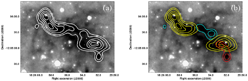
Figure 8: The NH₃ column density integrated over all velocities is shown in (a). The column density contribution of the separate velocity components is shown in (b). The separated velocity components are centered at 25.7 km s^-1 (blue), 26.7 km s^-1 (yellow), and 28.4 km s^-1 (red). Contours indicate $10^{15}$ cm^-2, $2\times 10^{15}$ cm^-2, and then increase in steps of $2\times 10^{15}$ cm^-2.

The NH₃ column density distribution is shown in Figure 8. The column densities lie in the range $10^{15}$ to $1.6\times 10^{16}$ cm^-2. In all three subclouds, there appears to be a lower density envelope ($\sim 10^{15}$ cm^-2) around higher density clumps ($\sim 4\times 10^{15}$ to $1.6\times 10^{16}$ cm^-2). The uncertainty in column density is $\lesssim 30$% within the clumps, but at the cloud boundaries the values are only good to approximately a factor of two. C1, C2, and C3 are coincident with column density peaks.

Pillai et al. (2006) found the [NH₃]/[H₂] abundance ratio in IRDCs ranged from $0.7\times 10^{-8}$ to $10\times 10^{-8}$. We assume a [NH₃]/[H₂] abundance ratio of $3\times 10^{-8}$ (Harju et al., 1993). The H₂ column densities imply peak $A_{V}\gtrsim 100$ (Bohlin et al., 1978; Schultz & Wiemer, 1975), in good agreement with the observed 8 $\mu$m absorption. To convert from column density to volume density, the line of sight depth must be determined. We assume a cylindrical geometry for the filamentary IRDC, with the semi-major axis (“length”) directed from the northeast corner to the southwest corner of the IRDC. We approximate the semi-minor axis (“width”) of the IRDC, aligned perpendicular to the semi-major axis, to be $\sim 0.35$ pc. The assumption of cylindrical geometry was then used to calculate the depth at each point in the IRDC. The calculated H₂ number densities then range from $\sim 3\times 10^{4}$ to $5\times 10^{5}$ cm^-3, values consistent with previous number densities reported for IRDCs (Carey et al., 1998; Egan et al., 1998; Pillai et al., 2006; Wang et al., 2008).

4.3 CCS Column Density

The CCS ($2_{1}-1_{0}$) column density, $N_{1}$, is determined using

$$N_{1}=\frac{8\pi^{1.5}\nu^{2}k}{hc^{3}}\frac{g_{1}}{g_{2}}\frac{1}{A_{21}}T_{b}\frac{\Delta V}{\sqrt{8\ln(2)}},$$ (6)

where the symbols are defined as in Equations 4 and 5. Equation 6 assumes the CCS ($2_{1}-1_{0}$) emission is optically thin and fills the synthesized beam. We assume $T_{b}\Delta V$ to be the integrated emission of the CCS over 1.2 km s^-1. Using the partition function $Q[T_{ex}]$, where $T_{ex}$ is the temperature describing the relative level populations, the total column density is obtained:

$$N_{total}=\frac{N_{1}Q[T_{ex}]}{g_{1}}\exp\biggl{[}\frac{E}{kT_{ex}}\biggr{]}.$$ (7)

where $E$ is the energy of the $1_{0}$ level above the ground state. Values for the partition function were interpolated from JPL line catalog values in the same manner as for NH₃ (Pickett et al., 1998). We assume a CCS $T_{ex}$ of 10 K based on typical values of NH₃ $T_{R}$ in areas where CCS was detected. Typical CCS column densities ranged from $10^{13}$ to $3\times 10^{13}$ cm^-2, roughly two orders of magnitude lower than the NH₃ column densities. Unfortunately, the unknown CCS $T_{ex}$ introduces significant uncertainty in the column density measurements; using an excitation temperature of 5 K reduces the column densities to $5\times 10^{12}$ to $10^{13}$ cm^-2, while 15 K produces column densities ranging from $2\times 10^{13}$ to $6\times 10^{13}$ cm^-2. Due to the large uncertainties in the CCS excitation temperature and linewidth, these CCS column densities are likely accurate to only an order of magnitude.

The CCS $T_{ex}$ can be constrained using CCS (4₃–3₂) observations of Sakai et al. (2008) (HPBW $\sim 37$″). Sakai et al. (2008) used a non-detection of CCS (4₃–3₂) emission to report an upper limit on the total CCS column density of $\lesssim 3.7\times 10^{12}$ cm^-2 at C1 and $\lesssim 3.5\times 10^{12}$ cm^-2 at C2. We used these results to derive an upper limit for the CCS (4₃–3₂) column density, $N_{3}$, at C1 and C2. To compare our observations with those of Sakai et al. (2008) we smoothed our CCS $N_{1}$ column density image to match the Nobeyama Radio Observatory resolution, FWHM 37″, and measured $N_{1}$ at the Sakai et al. (2008) pointings. By comparing our measured $N_{1}$ values and the $N_{3}$ upper limits and assuming local thermodynamic equilibrium, we derived a CCS $T_{ex}$ upper limit of $\lesssim 5$ K.

4.4 Mass

IRDC and clump masses were derived from NH₃ column densities. The mass of the IRDC was determined by integrating the NH₃ column density (shown in Fig. 8) over the entire source area (clumps as well as diffuse gas), giving the total number of NH₃ molecules in the IRDC. The number of molecules was converted to total mass by assuming the mass is dominated by H₂ and using the assumed [NH₃]/[H₂] abundance ratio of $3\times 10^{-8}$ (Harju et al., 1993) and an H₂ mass of $3.34\times 10^{-24}$ g. The IRDC mass is $\sim 1130$ M_☉, consistent with the $\sim 900$ M_☉ reported by Pillai et al. (2006). Rathborne et al. (2006) determined a total IRDC mass of $\sim 400$ M_☉ using 1.2 mm dust emission. The apparent discrepancy between the masses determined from NH₃ observations and dust observations may be attributed to the large systematic uncertainties in the dust emissivity, dust to gas ratio, and [NH₃]/[H₂] ratio.

The individual masses of C1, C2, C3, and C4 were calculated by integrating NH₃ column density over only the clumps’ spatial extents, and assuming an [NH₃]/[H₂] abundance ratio of $3\times 10^{-8}$. The clump radii were determined by fitting the NH₃ emission distribution in C1, C2, C3 and C4 with a 2-D Gaussian using AIPS task JMFIT and using the FWHMs as the radii of the clumps. Clumps C1, C2, C3, and C4 have masses 140, 160, 30, and 30 M_☉, respectively. The mass uncertainties given in Table 2 are based on uncertainty in the column densities and clump radii; it should be noted that uncertainties in the distance to the IRDC and the [NH₃]/[H₂] abundance ratio introduce additional systematic uncertainty. While the mass uncertainty may be quite large, Rathborne et al. (2006) determined masses of 113 M_☉ for C1 and 114 M_☉ for C2 using 1.2 mm dust emission. Rathborne et al. (2006) assumed a dust temperature of 15 K, comparable to the temperatures we have measured in this IRDC (mean $T_{K}\sim 17$ K, mean $T_{R}\sim 15$ K). The clump radii determined by Rathborne et al. (2006) were 0.15 pc for C1 and 0.21 pc for C2, comparable to the $\sim 0.1$ pc determined for C1 and C2 in this study. The Rathborne et al. (2006) masses are in good agreement with those found in this study, despite the fact that the overall IRDC mass determined by Rathborne et al. (2006) is a factor of three lower than that determined in this study. The fact that the masses agree on the scale of the clumps but not on the scale of the cloud may be due to sensitivity and/or resolution differences between the two studies.

5 Discussion

5.1 Clump stability

We examined the stability of C1, C2, C3, and C4 by comparing their gas mass to their virial masses. The virial mass ($M_{vir}$) is the mass at which thermal plus turbulent gas pressure balances gravitational forces in the clumps, i.e., the gravitational and kinetic energy are in equipartition. The ratio of virial mass and clump mass ($M_{vir}/M_{clump}$) is a basic indicator of whether the clumps are gravitationally bound and likely to collapse: if $M_{vir}/M_{clump}<1$, the clump contains enough mass to collapse under gravity. This balance analysis assumes negligible contributions to clump stability from additional forces such as magnetic fields and clump rotation, neither of which are known for the clumps in G19.30+0.07. Additionally, clump confinement by external pressure (Bertoldi & McKee, 1992) has not been included. We calculated $M_{vir}$ from the clump radius ($R_{clump}$, determined in §4.4) and the NH₃ FWHM linewidth ($\Delta V$) using

$$M_{vir}=\frac{15\Delta V^{2}R_{clump}}{8{\rm ln}(2)G}$$ (8)

The NH₃ (1,1) FWHM linewidth was measured at the density peak of the clumps. Values of $\Delta V$, $M_{vir}$, and $M_{vir}/M_{clump}$ are listed in Table 2.

The clumps all have $M_{vir}/M_{clump}>1$, inconsistent with indications of star formation that imply the clumps are undergoing gravitational collapse. However, Equation 8 assumes virial equilibrium. If the clumps have already collapsed and harbor outflows the conditions of virial equilibrium are violated, and the linewidths will not accurately predict the thermal and turbulent motion supporting the clumps. Indeed, clumps C1, C2, and C3 show evidence of outflow through either broad NH₃ linewidths or H₂O masers. Clump C4 has $M_{vir}/M_{clump}\sim 8$; this high ratio may be a result of increased linewidths toward C4 caused by the outflow originating from C2 (see §4.1). It is also worth noting that where the cores are optically thick the $\Delta V$ may be overestimated, which would lead to a greater overestimate of virial mass (which is proportional to $\Delta V^{2}$) than of clump mass (which is proportional to $\Delta V$).

The virial masses of C1 and C2 reported by Pillai et al. (2006) are 893 and 823 $M_{\sun}$, significantly larger than our $M_{vir}$ values. Pillai et al. (2006) used larger clump radii and higher linewidths in their virial mass calculations because of the lower resolution of their study (40″). Our higher resolution shows most of the mass is contained within a smaller radius than previously thought. Furthermore, we were able to resolve velocity gradients in the emission near the clumps (Fig. 4). The larger beam used by Pillai et al. (2006) would have confused this emission, contributing to their larger linewidth measurements.

5.2 The Relationship Between NH₃ and CCS

Chemical evolution models comparing CCS and NH₃ distributions have mainly been developed from observations of low mass star forming regions and the environs of H ii regions; we now examine whether such models might also apply in IRDCs. Chemical models such as those of Suzuki et al. (1992), Bergin & Langer (1997), and van Dishoeck & Blake (1998) predict that CCS traces chemically young gas in lower density, quiescent envelopes of molecular clouds, while NH₃ traces dense, evolved clumps. Time-dependent gas-phase modeling suggests that for low-mass star-forming clumps the [CCS]/[NH₃] abundance ratio is a measure of the age of clumps, i.e., a “chemical clock”: CCS abundance peaks in chemically young gas and decreases as the CCS components are reprocessed into molecules with stronger binding energies, such as CO. Millar & Herbst (1990) and Nejad & Wagenblast (1999) propose CCS is reprocessed on timescales of $\sim 10^{5}$ years, while de Gregorio-Monsalvo et al. (2005, 2006) concluded that CCS has a lifetime of $\sim 10^{4}$ years after the onset of star formation.

Freeze-out onto dust grains likely plays a significant role in chemical changes during clump evolution. Dust grain chemistry is particularly important for explaining the high abundances of NH₃ observed in dense clumps (Bergin & Langer, 1997; Bergin & Tafalla, 2007; Sakai et al., 2008). When CO freezes out onto dust grains the abundance of NH₃ is enhanced, because gas-phase CO destroys NH₃ parent molecules (Bergin & Langer, 1997). Furthermore, the abundance of hydrogenated molecules, including NH₃, may be enhanced as ices evaporate off dust grains (van Dishoeck & Blake, 1998) near hot clumps in star-forming regions. Freeze-out of CCS onto dust grains may also be responsible for low CCS abundances in gas clumps where $n_{\rm H_{2}}>10^{6}$ cm^-3 (Bergin & Langer, 1997). Dust grain chemistry also explains how the chemical clock may be reset. Dickens et al. (2001) propose collisions in gas with properties similar to IRDC subclouds can trigger MHD waves and/or grain impacts that provide sufficient energy for thermal desorption of molecules from grain surfaces, leading to the presence of early-time molecules like CCS.

The critical densities of the NH₃ (1,1) and CCS ($2_{1}-1_{0}$) emission lines differ by almost two orders of magnitude, $\sim 2\times 10^{3}$ cm^-3 for NH₃ (Danby et al., 1988) and $\sim 10^{5}$ cm^-3 for CCS (Wolkovitch et al., 1997), which can complicate the interpretation of molecular distribution. However, despite its higher critical density, we detect CCS emission in the lower density envelopes around the high-density NH₃ clumps rather than toward the center of the dense clumps, suggesting their spatial distributions are the result of chemical evolution in the IRDC rather than a density effect.

Previous studies of the chemistry in G19.30+0.07 have been limited by poor resolution. Prior to this investigation, Pillai et al. (2006) observed G19.30+0.07 in NH₃ emission using the Effelsberg 100 m telescope with 40″ resolution, but lacked the resolution needed to comment on small-scale structure. Sakai et al. (2008) observed N₂H⁺(1–0), HC₃N(5–4), CCS(4₃–3₂), CH₃OH(7–6), and NH₃ (1,1), (2,2), and (3,3) emission towards the clumps in G19.30+0.07 with the NRO 45-m telescope (HPBW $\sim 37$″ for CCS and $\sim 73$″ for NH₃). Sakai et al. (2008) report abundances suggesting the clumps in G19.30+0.07 are more chemically evolved than low-mass starless cores. The high spatial resolution data we present here improve upon these findings by showing how morphology, temperature, and density structure in the IRDC impact the distributions of the NH₃ and CCS.

Fig. 3 shows the integrated CCS emission in each of the subclouds and compares it to the NH₃ integrated emission. Although CCS emission is associated with the subclouds at 25.7 km s^-1, 26.7 km s^-1, and 28.4 km s^-1, the spatial distribution of the CCS and NH₃ emission are not coincident. Enhancements in the CCS with clump-like morphology are labeled as P1 to P5 in Fig. 3; no evidence of NH₃ clumps exist at these locations.

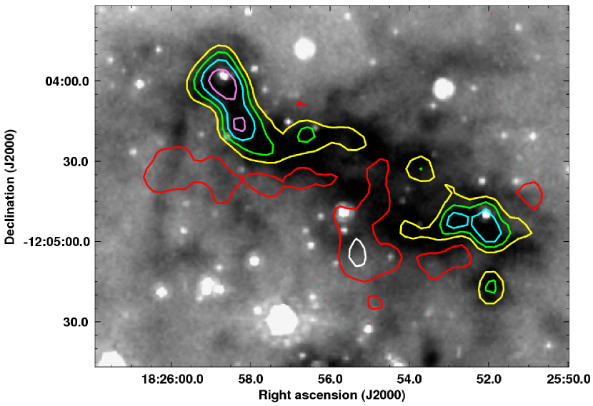
Figure 9: Column density ratio map showing the relative distribution of CCS and NH₃ ([CCS]/[NH₃]). Only areas with detectable emission from at least one of the molecules are mapped. In CCS peaks lacking detectable NH₃ emission we assign an NH₃ column density upper limit of $10^{15}$ cm^-2. Where NH₃ but no CCS was detected we assign a CCS column density upper limit of $10^{13}$ cm^-2. Contours scale logarithmically, with log([CCS]/[NH₃]) = $-$2.9 (violet), $-$2.7 (cyan), $-$2.5 (green), $-$2.3 (yellow), $-$1.9 (red), and $-$1.7 (white).

Typical CCS column densities ranged from $10^{13}$ cm^-2 to $3\times 10^{13}$ cm^-2. We examined the [CCS]/[NH₃] column density ratio in areas with detectable emission from at least one of the molecules. In CCS peaks lacking detectable NH₃ emission we assign an NH₃ column density upper limit of $10^{15}$ cm^-2. Where NH₃ but not CCS was detected we assign a CCS column density upper limit of $10^{13}$ cm^-2. At clumps C1, C2, C3, and C4 the [CCS]/[NH₃] ratio is $\lesssim 10^{-3}$, slightly higher than the upper limit determined by Sakai et al. (2008), and consistent with active, star forming clumps (Bergin & Tafalla, 2007; Sakai et al., 2008). At CCS emission peaks, [CCS]/[NH₃] ratios are $\gtrsim 0.02$, consistent with results from Suzuki et al. (1992), who found [CCS]/[NH₃] $\gtrsim 0.03$ in low-mass starless clumps. A map of the column density ratios is shown in Figure 9.

Comparing Fig. 9 with Fig. 3 shows that P1 is associated with the [CCS]/[NH₃] peak and located in the subcloud located at 25.7 km s^-1, the only subcloud lacking evidence of star formation. The CCS morphology and [CCS]/[NH₃] ratio in this subcloud are consistent with a chemically young clump in a stage too early to present evidence of star formation (de Gregorio-Monsalvo et al., 2006).

The CCS peaks P2, P4, and P5 are located at subcloud interfaces, and P3 is spatially coincident with the outflow from C2. The spatial coincidence of these CCS peaks with subcloud-subcloud and outflow-subcloud interfaces indicates collisions may be resetting the chemical clock of the gas at these locations, consistent with the Dickens et al. (2001) model.

One major caveat must be considered in the analysis of CCS emission. CCS ($2_{1}-1_{0}$) is a low-lying energy state transition (upper energy level only 1.6 K above ground), so it is difficult to know whether enhanced CCS emission is due to excitation effects or increased abundance. Using the results of Sakai et al. (2008) we were able to roughly constrain the CCS excitation temperature to $\lesssim 5$ K. However, the CCS ($4_{3}-3_{2}$) observations were low resolution and only provided a column density upper limit. Additional transitions of CCS must be measured at comparable resolution to this study to more accurately determine the CCS excitation temperature. Sensitive interferometric observations at millimeter wavelengths could explore whether the abundance measurements in the ground state are consistent with abundances measured from higher energy transitions.

We draw the following conclusions from the CCS detections: (1) CCS and NH₃ are present in each of the three subclouds comprising G19.30+0.07, but each molecule traces different parts of the subclouds; (2) CCS appears to trace the boundaries of the IRDC while NH₃ peaks in the inner parts of the IRDC, consistent with CCS enhancement in low-density envelopes and NH₃ enhancement in denser clumps, in spite of the fact that the CCS transition has the higher critical density. This emphasizes that NH₃ does not give the full picture of the dense gas in star-forming regions; (3) in some cases, CCS appears to have clump-like morphology. The [CCS]/[NH₃] peak at P1 is located in the only subcloud lacking evidence of star formation. This supports the hypothesis that CCS cores may represent the very earliest stages of core formation; (4) CCS peaks at subcloud-subcloud or outflow-subcloud interfaces may indicate collisions are resetting the chemical clock in some parts of the IRDC; and (5) further investigations at higher-energy transitions are needed to distinguish excitation and abundance effects in CCS emission.

5.3 Star Formation in G19.30+0.07

Although early studies of G19.30+0.07 did not find any evidence of star formation (Carey et al., 1998), recent investigations, including this one, indicate substantial active star formation in this IRDC. The observed evidence for star formation is: (1) archival MIPSGAL 24 $\mu$m observations showing areas of hot dust associated with C1, C2, and S1; (2) structure in the NH₃ spectral line observations consistent with outflows originating from C1 and C2; (3) H₂O masers coincident with C3 and S1 (Fig. 1).

No 8.4 GHz continuum emission was detected in the IRDC. A 5$\sigma$ detection limit of 0.125 mJy beam^-1 sets the upper limit of the UV photon flux at $<8\times 10^{43}$ s^-1, implying a stellar type of B3 or later (Smith et al., 2002; Panagia, 1973). However, if the protostar is accreting material, much of the stellar UV radiation will be absorbed close to the star (Churchwell, 1997). Also, in an IRDC it is likely that some UV photons are absorbed by dust. Thus, stars with types hotter than B3 could be present in G19.30+0.07 but be undetected by our measurements. In fact, Orion Source I, an early-B star with mass $\gtrsim 8$ M_☉ (Matthews et al., 2010), has an 8.4 GHz flux density of $\sim 1.1$ mJy (Menten & Reid, 1995) at a distance of $\sim 400$ pc (Menten et al., 2007). If Orion Source I were located at the distance of G19.30+0.07, 2.4 pc, its flux density would be only $\sim 0.03$ mJy, below the detection limit of this study.

Clump masses of $\geq 10^{2}$ M_☉ and the presence of outflows suggest that C1 and C2 may be protoclusters. Using the initial mass function from Scalo (1986) and assuming a 50% star forming efficiency, these clumps would form stars up to masses of $\sim 3$ M_☉. The smaller NH₃ clump and H₂O maser without accompanying 24 $\mu$m emission at C3 suggest C3 likely contains protostars that are either lower-mass or younger than those in C1 and C2. The 24 $\mu$m emission toward S1 suggests the presence of at least one protostar, consistent with the H₂O maser coincident with S1. It may be S1 is more evolved than C1 and C2, and has destroyed or dispersed any dense gas associated with its formation. However, no shell of dispersed NH₃ is detected around S1.

Assuming the linewing structure discussed in §4.2 indicates outflows, the outflow masses provide insight into the masses of the stars contained in C1 and C2. The column densities in the outflows were determined as in Equations 6 and 7, using the integrated emission from the NH₃ (2,2) line-wings and assuming a $T_{ex}$ of 10 K for NH₃. The column densities were summed over the outflow area to determine the masses of the outflows. The red and blue outflow components of C1 each contain $\sim 2$ M_☉ and the components in C2 each contain $\sim 1.6$ M_☉, suggesting intermediate or high mass protostar progenitors. However, we note that NH₃ only traces high density gas, so observations of the low-density gas are needed to better constrain the total outflow masses.

Various models attempt to explain the formation of massive stars, but recent work suggests accretion in turbulent clumps is the likely creation mechanism (Beuther et al., 2007). Beuther et al. (2007) present an evolutionary sequence of massive stars starting from high mass starless clumps: low- and intermediate-mass protostars form within the massive starless clumps and accrete matter until becoming a massive protostellar object, which develops into a massive star and clears the natal gas from its environment. C1 and C2 may be examples of clumps containing the embedded accreting protostars proposed in this model.

Based on the results from this single IRDC, the role that subclouds play in massive protostar and protocluster development is still unclear. They may indicate an early stage of fragmentation, cloud formation/collision, or a superposition along the line of sight. The subclouds appear distinct, but if less dense gas below our detection limits connects the subclouds, they may all be part of a larger structure. Further work is needed to understand the role of subclouds in IRDCs.

5.4 Is G19.30+0.07 a “Typical” IRDC?

Understanding the role of IRDCs in star formation requires a survey of their properties. We have examined one IRDC in great detail, but is G19.30+0.07 a typical IRDC, and how general are our findings? Our results are consistent with previous studies that indicate G19.30+0.07 has temperatures and densities typical for an IRDC (Carey et al., 1998; Pillai et al., 2006; Wang et al., 2008; Rathborne et al., 2006). The high resolution of this study compared to previous work has revealed new IRDC features. Notably, the kinematics have been analyzed in detail. We find that the IRDC is composed of three subclouds, each of which has a slightly different velocity. The universality of multiple subclouds in IRDCs and the role they play in protocluster evolution requires further investigation.

6 Conclusions

Massive star formation continues to be poorly understood, largely because early stages are difficult to observe due to the short timescales involved and the embedded nature of massive protostars. Because of their large masses, low temperatures, and high densities, IRDCs are currently the most likely candidates to host the first stages of massive star formation. Understanding their properties may shed light on the processes that lead to the creation of massive protostars. Although IRDCs are identified using IR observations, their high opacity makes radio wavelengths an important probe of their structure. We have examined IRDC G19.30+0.07 using VLA spectral line observations of the NH₃ (1,1), (2,2), and CCS ($2_{1}-1_{0}$) transitions. From this work, we draw the following conclusions:

1. G19.30+0.07 has structure down to the resolution limit of our observations (4″ to 6″). At a distance of 2.4 kpc, the structure is $\lesssim 1.4\times 10^{4}$ AU in size. This level of detail is seen in the IR images as well as the NH₃ and CCS observations.

2. G19.30+0.07 is composed of three subclouds at different velocities. Star formation and [CCS]/[NH₃] levels may indicate that one of the subclouds is at an earlier evolutionary stage than the other two. Further investigation is needed to determine if IRDCs are typically composed of multiple subclouds, and the role subclouds play in IRDC evolution.

3. Typical values of $T_{R}$ in G19.30+0.07 range from 10 to 30 K with a mean value of $15\pm 3$ K. Increases in $T_{R}$ at C1, C2, and S1 indicate heat sources at these locations.

4. NH₃ column densities in G19.30+0.07 are $\sim 10^{15}$ to $1.6\times 10^{16}$ cm^-2, with lower density envelopes around higher density clumps.

5. The NH₃-derived masses of C1, C2, C3, and C4 are $140\pm 20$, $160\pm 40$, $30\pm 20$, and $30\pm 20$ M_☉. The clumps have masses significantly lower than their virial masses; however, signs of star formation indicate C1, C2, and C3 are gravitationally bound and collapsing. In clumps that are collapsing or contain outflows, $M_{virial}/M_{core}$ is not a reliable metric for testing gravitational boundedness.

6. CCS and NH₃ are present in each of the three subclouds comprising G19.30+0.07, and appear to trace different parts of the subclouds. The NH₃ emission closely traces the IR extinction seen in the GLIMPSE 8 $\mu$m images, and peaks where clumps are forming and evolving in the IRDC. Conversely, the CCS tends to trace the boundaries of the IRDC, where NH₃ column densities indicate the IRDC is more diffuse. Given the high critical density of CCS ($\sim 10^{5}$) (Wolkovitch et al., 1997), the CCS detections at the IRDC boundaries demonstrate that NH₃ does not give the full picture of the dense gas in star-forming regions.

7. In some places, the CCS appears to have clump-like morphology. The CCS peaks may show the very earliest stages of clump formation and/or result from collisions that reset the chemical clock of the gas.

8. Stars are forming in G19.30+0.07, most obviously in clumps C1 and C2. Younger or lower mass clumps may look like C3, where a H₂O maser but no IR emission is present, or C4, where no signs of star formation have yet been detected. S1, where a H₂O maser coincides with a 24 $\mu$m source but no NH₃ clump is detected, may be a more evolved protostar, or associated with NH₃ at a velocity outside our observed bandwidth. We did not detect 8.4 GHz emission from the IRDC, although the 8.4 GHz emission from the early-B star Orion Source I would be below our detection limits if it were at a distance of 2.4 kpc.

7 Acknowledgments

KD thanks the NRAO pre-doctoral research program for support and funding. EC and KD were also supported during this work by the National Science Foundation under grants AST-0303689 and AST-0808119. During this investigation RI was supported by a Spitzer Fellowship to the University of Virginia and by JPL/Spitzer grants RSA 1276990 and RSA 127546. The authors thank the anonymous referee for his or her insightful comments and careful reading of the text.

Table 1: VLA Observation Details

Parameter	NH3 (1,1)	NH3 (2,2)	CCS ($2_{1}-1_{0}$)	8.4 GHz
Observation Date	2005 Dec 10, 11	2005 Dec 10, 11	2007 Feb 19	2006 Jan 30
NRAO Proposal ID	AD516	AD516	AD556	AD524
Rest Frequency (GHz)	23.6944955	23.7226333	22.3440330	8.4351
VLA Configuration	D	D	D	A
Total Bandwidth (MHz)	3.125	3.125	3.125	50
Number of channels	128	128	128	1
Spectral Resolution (kHz/km s-1)	24.4/0.3	24.4/0.3	24.4/0.3	$\cdots$
Primary Beam FWHM	1.9′	1.9′	1.9′	5.3′
Synthesized Beam	4$\farcs$5$\times$3$\farcs$4	4$\farcs$6$\times$3$\farcs$4	7$\farcs$7$\times$5$\farcs$7	0$\farcs$31$\times$0$\farcs$19
RMS Noise (mJy beam-1 channel-1)	4.5	4.5	3	0.003
Beam Position Angle	4.8∘	$-$0.6∘	6.7∘	20.1∘
Conversion Factor (K/Jy)	144	138	55.7	2.9 $\times 10^{5}$
Smoothed Synthesized Beam	6$\farcs$0$\times$6$\farcs$0	6$\farcs$0$\times$6$\farcs$0	$\cdots$	$\cdots$
Smoothed Beam Position Angle	0∘	0∘	$\cdots$	$\cdots$
RMS Noise (Smoothed Data, mJy beam-1 channel-1)	6	6	$\cdots$	$\cdots$
Smoothed Conversion Factor (K/Jy)	60.5	60.3	$\cdots$	$\cdots$
Largest Detectable Angular Scale	94″	94″	100″	16″
Phase and Amplitude Calibrator	J1832$-$105	J1832$-$105	J1832$-$105	J1832$-$105
Flux Density Calibrator	3C48	3C48	3C286	3C48
Bandpass Calibrator	3C273	3C273	3C345	$\cdots$

Table 2: NH₃ Clump Properties

	C1	C2	C3	C4
$M_{\rm clump}$ (H2) (M☉)	$140\pm 20$	$160\pm 40$	$30\pm 20$	$30\pm 20$
$M_{\rm clump}$ (dust) (M☉)	113	114	$\cdots$	$\cdots$
$R_{\rm clump}$ (pc)	$0.11\pm 0.002$	$0.12\pm 0.003$	$0.07\pm 0.006$	$0.09\pm 0.005$
$\Delta V$ (km s-1)	$2.8\pm 0.1$	$1.8\pm 0.1$	$1.6\pm 0.1$	$2.1\pm 0.2$
$M_{\rm virial}$ (M☉)	$540\pm 50$	$260\pm 40$	$110\pm 20$	$240\pm 40$
$M_{\rm virial}$/$M_{\rm clump}$	$4\pm 1$	$2\pm 1$	$4\pm 2$	$8\pm 5$

References

- Bachiller et al. (1987) Bachiller, R., Guilloteau, S., & Kahane, C. 1987, A&A, 173, 324
- Benjamin et al. (2003) Benjamin, R. A., et al. 2003, PASP, 115, 953
- Bergin & Tafalla (2007) Bergin, E. A., & Tafalla, M. 2007, ARA&A, 45, 339
- Bergin & Langer (1997) Bergin, E. A., & Langer, W. D. 1997, ApJ, 486, 316
- Beuther et al. (2007) Beuther, H., Churchwell, E. B., McKee, C. F., & Tan, J. C. 2007, Protostars and Planets V, 165
- Bertoldi & McKee (1992) Bertoldi, F., & McKee, C. F. 1992, ApJ, 395, 140
- Bohlin et al. (1978) Bohlin, R. C., Savage, B. D., & Drake, J. F. 1978, ApJ, 224, 132
- Carey et al. (1998) Carey, S. J., Clark, F. O., Egan, M. P., Price, S. D., Shipman, R. F., & Kuchar, T. A. 1998, ApJ, 508, 721
- Carey et al. (2009) Carey, S. J., et al. 2009, PASP, 121, 76
- Churchwell (1997) Churchwell, E. 1997, ApJ, 479, L59
- Churchwell et al. (2009) Churchwell, E., et al. 2009, PASP, 121, 213, E. 2002, ARA&A, 40, 27
- Condon (1992) Condon, J. J. 1992, ARA&A, 30, 575
- Danby et al. (1988) Danby, G., Flower, D. R., Valiron, P., Schilke, P., & Walmsley, C. M. 1988, MNRAS, 235, 229
- de Gregorio-Monsalvo et al. (2005) de Gregorio-Monsalvo, I., Chandler, C. J., Gómez, J. F., Kuiper, T. B. H., Torrelles, J. M., & Anglada, G. 2005, ApJ, 628, 789
- de Gregorio-Monsalvo et al. (2006) de Gregorio-Monsalvo, I., Gómez, J. F., Suárez, O., Kuiper, T. B. H., Rodríguez, L. F., & Jiménez-Bailón, E. 2006, ApJ, 642, 319
- Dickens et al. (2001) Dickens, J. E., Langer, W. D., & Velusamy, T. 2001, ApJ, 558, 693
- Egan et al. (1998) Egan, M. P., Shipman, R. F., Price, S. D., Carey, S. J., Clark, F. O., & Cohen, M. 1998, ApJ, 494, L199
- Goldsmith & Langer (1999) Goldsmith, P. F., & Langer, W. D. 1999, ApJ, 517, 209
- Harju et al. (1993) Harju, J., Walmsley, C. M., & Wouterloot, J. G. A. 1993, A&AS, 98, 51
- Ho & Townes (1983) Ho, P. T. P., & Townes, C. H. 1983, ARA&A, 21, 239
- Indebetouw et al. (2005) Indebetouw, R., et al. 2005, ApJ, 619, 931
- Matthews et al. (2010) Matthews, L. D., Greenhill, L. J., Goddi, C., Chandler, C. J., Humphreys, E. M. L., & Kunz, M. W. 2010, ApJ, 708, 80
- Menten & Reid (1995) Menten, K. M., & Reid, M. J. 1995, ApJ, 445, L157
- Menten et al. (2007) Menten, K. M., Reid, M. J., Forbrich, J., & Brunthaler, A. 2007, A&A, 474, 515
- Mezger & Henderson (1967) Mezger, P. G., & Henderson, A. P. 1967, ApJ, 147, 471
- Millar & Herbst (1990) Millar, T. J., & Herbst, E. 1990, A&A, 231, 466
- Nejad & Wagenblast (1999) Nejad, L. A. M., & Wagenblast, R. 1999, A&A, 350, 204
- Panagia (1973) Panagia, N. 1973, AJ, 78, 929
- Peretto & Fuller (2009) Peretto, N., & Fuller, G. A. 2009, A&A, 505, 405
- Pickett et al. (1998) Pickett, H. M., Poynter, I. R. L., Cohen, E. A., Delitsky, M. L., Pearson, J. C., & Muller, H. S. P. 1998, Journal of Quantitative Spectroscopy and Radiative Transfer, 60, 883
- Pillai et al. (2006) Pillai, T., Wyrowski, F., Menten, K. M., & Krügel, E. 2006, A&A, 447, 929
- Pillai et al. (2007) Pillai, T., Wyrowski, F., Hatchell, J., Gibb, A. G., & Thompson, M. A. 2007, A&A, 467, 207
- Rathborne et al. (2006) Rathborne, J. M., Jackson, J. M., & Simon, R. 2006, ApJ, 641, 389
- Rathborne et al. (2007) Rathborne, J. M., Simon, R., & Jackson, J. M. 2007, ApJ, 662, 1082
- Redman et al. (2003) Redman, R. O., Feldman, P. A., Wyrowski, F., Côté, S., Carey, S. J., & Egan, M. P. 2003, ApJ, 586, 1127
- Rydbeck et al. (1977) Rydbeck, O. E. H., Sume, A., Hjalmarson, A., Ellder, J., Ronnang, B. O., & Kollberg, E. 1977, ApJ, 215, L35
- Sakai et al. (2008) Sakai, T., Sakai, N., Kamegai, K., Hirota, T., Yamaguchi, N., Shiba, S., & Yamamoto, S. 2008, ApJ, 678, 1049
- Scalo (1986) Scalo, J. M. 1986, Fund. Cosmic Phys., 11, 1
- Schultz & Wiemer (1975) Schultz, G. V., & Wiemer, W. 1975, A&A, 43, 133
- Smith et al. (2002) Smith, L. J., Norris, R. P. F., & Crowther, P. A. 2002, MNRAS, 337, 1309
- Suzuki et al. (1992) Suzuki, H., Yamamoto, S., Ohishi, M., Kaifu, N., Ishikawa, S.-I., Hirahara, Y., & Takano, S. 1992, ApJ, 392, 551
- Tafalla et al. (2004) Tafalla, M., Myers, P. C., Caselli, P., & Walmsley, C. M. 2004, A&A, 416, 191
- van Dishoeck & Blake (1998) van Dishoeck, E. F., & Blake, G. A. 1998, ARA&A, 36, 317
- Wang et al. (2006) Wang, Y., Zhang, Q., Rathborne, J. M., Jackson, J., & Wu, Y. 2006, ApJ, 651, L125
- Wang et al. (2008) Wang, Y., Zhang, Q., Pillai, T., Wyrowski, F., & Wu, Y. 2008, ApJ, 672, L33
- Wolkovitch et al. (1997) Wolkovitch, D., Langer, W. D., Goldsmith, P. F., & Heyer, M. 1997, ApJ, 477, 241