DB Category: Denotational Semantics for View-based Database Mappings

Abstract

We present a categorical denotational semantics for a database mapping, based on views, in the most general framework of a database integration/exchange. Developed database category $~{}DB~{}$, for databases (objects) and view-based mappings (morphisms) between them, is different from $Set$ category: the morphisms (based on a set of complex query computations) are not functions, while the objects are database instances (sets of relations). The logic based schema mappings between databases, usually written in a highly expressive logical language (ex. LAV, GAV, GLAV mappings, or tuple generating dependency) may be functorially translated into this ”computation” category $DB$. A new approach is adopted, based on the behavioral point of view for databases, and behavioral equivalences for databases and their mappings are established. By introduction of view-based observations for databases, which are computations without side-effects, we define a fundamental (Universal algebra) monad with a power-view endofunctor $T$. The resulting 2-category $DB$ is symmetric, so that any mapping can be represented as an object (database instance) as well, where a higher-level mapping between mappings is a 2-cell morphism. Database category $DB$ has the following properties: it is equal to its dual, complete and cocomplete. Special attention is devoted to practical examples: a query definition, a query rewriting in GAV Database-integration environment, and the fixpoint solution of a canonical data-integration model.

1 Introduction

Most work in the data integration/exchange and P2P framework is based on a logical point of view (particularly for the integrity constraints, in order to define the right models for certain answers) in a ’local’ mode (source-to-target database), where a general ’global’ problem of a composition of complex partial mappings that involves a number of databases has not been given the correct attention. Today, this ’global’ approach cannot be avoided because of the necessity of P2P open-ended networks of heterogenous databases. The aim of this work is a definition of category $DB$ for database mappings more suitable than a $Set$ category: The databases are more complex structures w.r.t. sets, and the mappings between them are too complex to be represented by a single (complete) function. Why do we need an enriched categorical semantic domain such as this for databases? We will try to give a simple answer to this question:
-     This work is an attempt to give a correct solution for a general problem of complex database-mappings and for high level algebra operators for databases (merging, matching, etc.), preserving the traditional common practice logical language for schema database mapping definitions.
-     The query-rewriting algorithms are not integral parts of a database theory (used to define a database schema with integrity constraints); they are programs and we need an enriched context that is able to formally express these programs trough mappings between databases as well.
-      Let us consider, for example, P2P systems or mappings in a complex Datawarehouse: formally, we would like to make a synthetic graphic representations of database mappings and queries and to develop a graphic tool for a meta-mapping description of complex (and partial) mappings in various contexts, with a formal mathematical background.
Only a few works considered this general problem  [1, 2, 3, 4]. One of them, which uses a category theory  [2], is too restrictive: their institutions can be applied only for inclusion mappings between databases.
There is a lot of work for sketch-based denotational semantics for databases [5, 6, 7, 8]. But all of them use, as objects of a sketch category, the elements of an ER-scheme of a database (relations, attributes, etc..) and not the whole database as a single object, which is what we need in a framework of inter-databases mappings. It was shown in [9] that if we want to progress to more expressive sketches w.r.t. the original Ehresmann’s sketches for diagrams with limits and coproducts, by eliminating non-database objects as, for example, cartesian products of attributes or powerset objects, we need more expressive arrows for sketch categories (diagram predicates in [9] that are analog to the approach of Makkai in [10]). Obviously, when we progress to a more abstract vision where objects are the (whole) databases, following the approach of Makkai, in this new basic category $DB$ for databases, where objects are just the database instances (each object is a set of relations that compose this database instance), we will obtain much more complex arrows, as we will see. Such arrows are not simple functions, as in the case of base $Set$ category, but complex trees (operads) of view-based mappings. In this way, while Ehresmann’s approach prefers to deal with few a fixed diagram properties (commutativity, (co)limitness), we enjoy the possibility of setting full relational-algebra signature of diagram properties.
This work is an attempt to give a correct solution for this problem while preserving the traditional common practice logical language for the schema database mapping definitions. Different properties of this DB category are considered in a number of previously published papers [11, 12, 13, 14, 15] as well.
This paper follows the following plan: In Section 2 we present an Abstract Object Type based on view-based observations. In Section 3 we develop a formal definition for a Database category $DB$, its power-view endofunctor, and its duality property. In Section 4 we formulate the two equivalence relations for databases (objects in $DB$ category): a strong and a weak observation equivalences. Finally, in Section 5 we present an application of this theory to the data integration/exchange systems, with an example for a query-rewriting in data integration system, and we define a fixpoint operator for an infinite canonical solution in data integration/exchange systems.

1.1 Technical Preliminaries

The database mappings, for a given logical language, are defined usually at a schema level, as follows:

• A database schema is a pair $\mathcal{A}=(S_{h},S_{n})$ where: $S_{h}$ is a countable set of relation symbols $r\in R$ with finite arity, disjoint from a countable infinite set att of attributes (for any $\textbf{x}\in\textbf{att}$ a domain of x is a nonempty subset $dom(\textbf{x})$ of a countable set of individual symbols dom, disjoint from att ), such that for any $r\in R$, the sort of $R$ is a finite sequence of elements of att. $S_{n}$ denotes a set of closed formulas called integrity constraints, of the sorted first-order language with sorts att, constant symbols dom, relational symbols $R$, and no function symbols.
  A finite database schema is composed by a finite set $S_{h}$, so that the set of all attributes of such a database is finite.

• An instance of a database $\mathcal{A}$ is given by $A=(\mathcal{A},I_{A})$, where $I_{A}$ is an interpretation function that maps each schema element of $S_{h_{A}}$ (n-ary predicate) into an n-ary relation $a_{i}\in A$ (called also ”element of $A$” ). Thus, a relational instance-database $A$ is a set of n-ary relations.

• We consider a rule-based conjunctive query over a database schema $\mathcal{A}$ as an expression $q(\textbf{x})\longleftarrow R_{1}(u_{1}),...,R_{n}(u_{n})$, where $n\geq 0$, $R_{i}$ are the relation names (at least one) in $\mathcal{A}$ or the built-in predicates (ex. $\leq,=,$ etc..), $q$ is a relation name not in $\mathcal{A}$, $u_{i}$ are free tuples (i.e., may use either variables or constants). Recall that if $v=(v_{1},..,v_{m})$ then $R(v)$ is a shorthand for $R(v_{1},..,v_{m})$. Finally, each variable occurring in x must also occur at least once in $u_{1},...,u_{n}$. Rule-based conjunctive queries (called rules) are composed by: a subexpression $R_{1}(u_{1}),....,R_{n}(u_{n})$, that is the body, and $q(\textbf{x})$ that is the head of this rule. If one can find values for the variables of the rule, such that the body holds (i.e. is logically satisfied), then one may deduce the head-fact. This concept is captured by a notion of ”valuation”. In the rest of this paper a deduced head-fact will be called ”a resulting view of a query $q(\textbf{x})$ defined over a database $\mathcal{A}$”. Recall that the conjunctive queries are monotonic and satisfiable. The $Yes/No$ conjunctive queries are the rules with an empty head.

• We consider that a mapping between two databases $\mathcal{A}$ and $\mathcal{B}$ is expressed by an union of ”conjunctive queries with the same head”. Such mappings are called ”view-based mappings”. Consequently we consider a view of an instance-database $A$ an n-ary relation (set of tuples) obtained by a ”select-project-join + union” (SPJRU) query $q(\textbf{x})$ (it is a term of SPJRU algebra) over $A$: if this query is a finite term of this algebra than it is called a ”finitary view” (a finitary view can have also an infinite number of tuples).

We consider the views as a universal property for databases: they are the possible observations of the information contained in an instance-database, and we may use them in order to establish an equivalence relation between databases. Database category $DB$, which will be introduced in what follows, is at an instance level, i.e., any object in $DB$ is an instance-database (i.e., a set of relations). The connection between a logical (schema) level and this computational category is based on the interpretation functors. Thus, each rule-based conjunctive query at schema level over a database $\mathcal{A}$ will be translated (by an interpretation functor) in a morphism in $DB$, from an instance-database $A$ (a model of the database schema $\mathcal{A}$) to the instance-database composed by all views of $A$.
In what follows we will work with the typed operads, first developed for a purpose of homotopy theory  [16, 17, 18], having a set $R$ of types (each relation symbol is a type), or ”R-operads” for short. The basic idea of an R-operad $O$ is that, given types $r_{1},...,r_{k},r\in R$, there is a set $O(r_{1},...,r_{k},r)$ of abstract $k\_ary$ ”operations” with inputs of type $r_{1},...,r_{k}$ and output of type $r$. We can visualize such an operation as a tree with only one node. In an operad, we can obtain new operations from old ones by composing them: it can be visualized in terms of trees (Fig. 1)

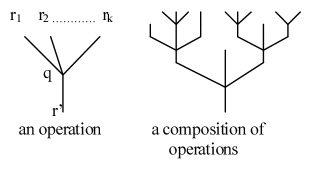
Figure 1: Operations of an R-operad

We can obtain the new operators from old ones by permuting arguments, and there is a unary ”identity” operation of each type. Finally, we insist on a few plausible axioms: the identity operations act as identities for composition, permuting arguments is compatible with composition, and composition is associative. Thus, formally, we have the following:

Definition 1

For any set R, an R-operad O consists of

1. for any $r_{1},...,r_{k},r\in R$, a set $O(r_{1},...,r_{k},r)$

2. for any $f\in O(r_{1},...,r_{k},r)$ and any $g_{1}\in O(r_{11},...,r_{1i_{1}},r_{1})$,…, $g_{k}\in O(r_{k1},...,r_{ki_{k}},r_{k})$, an element $f\cdot(g_{1},...,g_{k})\in O(r_{11},...,r_{1i_{1}},...,r_{k1},...,r_{ki_{k}},r)$

3. for any $r\in O$, an element $1_{r}\in O(r,r)$

4. for any permutation $\sigma\in R_{k}$, a map $\sigma:O(r_{1},...,r_{k},r)\rightarrow O(r_{\sigma(1)},...,r_{\sigma(k)},r)$, $f\longmapsto f\sigma$, such that:

   1. whenever both sides make sense, $f\cdot(g_{1}\cdot(h_{11},...,h_{1i_{1}}),..,.g_{k}\cdot(h_{k1},...,h_{ki_{k}}))=(f\cdot(g_{1},..,g_{k}))\cdot(h_{11},...,h_{1i_{1}},..,h_{k1},...,h_{ki_{k}})$

   2. for any $f\in O(r_{1},...,r_{k},r)$, $~{}f=1_{r}\cdot f=f\cdot(1_{r1},...,1_{rk})$

   3. for any $f\in O(r_{1},...,r_{k},r)$, and $\sigma,\sigma_{1}\in R_{k}$, $~{}f(\sigma\sigma_{1})=(f\sigma)\sigma_{1}$

   4. for any $f\in O(r_{1},...,r_{k},r)$, $~{}\sigma\in R_{k}$ and $g_{1}\in O(r_{11},...,r_{1i_{1}},r_{1})$,…,
      $g_{k}\in O(r_{k1},...,r_{ki_{k}},r_{k})$, $~{}(f\sigma)\cdot((g_{\sigma(1)},...,g_{\sigma(k)})=(f\cdot(g_{1},..,g_{k}))\rho(\sigma)$
      where $\rho:R_{k}\longrightarrow R_{i_{1}+...+i_{k}}$ is the obvious homomorphism.

   5. for any $f\in O(r_{1},...,r_{k},r)$, $~{}g_{1}\in O(r_{11},...,r_{1i_{1}},r_{1})$,..,$g_{k}\in O(r_{k1},...,r_{ki_{k}},r_{k})$, and $\sigma_{1}\in R_{i_{1}},....,\sigma_{k}\in R_{i_{k}}$, $~{}(f\cdot(g_{1}\sigma_{1},...g_{k}\sigma_{k}))=(f\cdot(g_{1},..,g_{k}))\varrho_{1}(\sigma_{1},...,\sigma_{k})$,
      where $\varrho_{1}:R_{i_{1}}\times...\times R_{i_{k}}\longrightarrow R_{i_{1}+...+i_{k}}$ is the obvious homomorphism.

Let us define the ”R-algebra” of an operad where its abstract operations are represented by actual functions (query-functions). For a given database schema with relation symbols $r_{1},...,r_{k}$ we consider $f\in O(r_{1},...,r_{k},r)$ as a conjunctive query $r\leftarrow r_{1},...,r_{k}$ that defines a view $r$.

Definition 2

For any R-operad O, a R-algebra $\alpha$ consists of:

1. for any $r\in R$, a set $\alpha(r)$ is a set of tuples of this type (relation). $~{}\alpha^{*}~{}$ is the extension of $\alpha~{}$ to a list of symbols $~{}\alpha^{*}(\{r_{1},...,r_{k}\})\triangleq\{\alpha(r_{1}),...,\alpha(r_{k})\}$.

2. for any $q\in O(r_{1},...,r_{k},r)$ a mapping function $\alpha(q):\alpha(r_{1})\times...\times\alpha(r_{k})\longrightarrow\alpha(r)$, such that

   1. whenever both sides make sense, $\alpha(q\cdot(q_{1},..,q_{k}))=\alpha(q)(\alpha(q_{1})\times...\times\alpha(q_{k}))$

   2. for any $r\in R$, $\alpha(1_{r})$ acts as an identity on $\alpha(r)$

   3. for any $q\in O(r_{1},...,r_{k},r)$ and a permutation $\sigma\in R_{k}$, $\alpha(q\sigma)=\alpha(q)\sigma$, where $\sigma$ acts on the function $\alpha(q)$ on the right by permuting its arguments.

3. we introduce the two functions, $\partial_{0}~{}and~{}\partial_{1}$, such that for any $\alpha(q)$, $~{}q\in O(r_{1},...,r_{k},r)$, we have that $\partial_{0}(q)=\{r_{1},...,r_{k}\}$, $~{}\partial_{0}(\alpha(q))=\{\alpha(r_{1}),...,\alpha(r_{k})\}$, $~{}\partial_{1}(q)=\{r\}$, and $\partial_{1}(\alpha(q))=\{\alpha(r)\}$.

Consequently, we can think of an operad as a simple sort of theory, used to define a schema mappings between databases, and its algebras as models of this theory used to define the mappings between instance-databases, where a mapping $\alpha$ is considered as an interpretation of relation symbols of a given database schema.

2 Data Object Type for query-answering database systems

We consider the views as a universal property for databases: they are the possible observations of the information contained in an instance-database, and we can use them in order to establish an equivalence relation between databases.
In a theory of algebraic specifications an Abstract Data Type (ADT) is specified by a set of operations (constructors) that determine how the values of the carrier set are built up, and by a set of formulae (in the simplest case, equations) stating which values should be identified. In the standard initial semantics, the defining equations impose a congruence on the initial algebra. Dually, a coagebraic specification of a class of systems, i.e., Abstract Object Types (AOT), is characterized by a set of operations (destructors) that specify what can be observed out of a system-state (i.e., an element of the carrier), and how a state can be transformed to a successor-state.
We start by introducing the class of coalgebras for database query-answering systems for a given instance-database (a set of relations) $A$. They are presented in an algebraic style, by providing a co-signature. In particular, the sorts include one single ”hidden sort” corresponding to the carrier of the coalgebra, and other ”visible” sorts, for inputs and outputs, that have a given fixed interpretation. Visible sorts will be interpreted as sets without any algebraic structure defined on them. For us, coalgebraic terms, built only over destructors, are precisely interpreted as the basic observations that one can make on the states of a coalgebra.
Input sorts are considered as a set $\mathcal{L}_{A}$ of union of conjunctive queries $q(\textbf{x})$ for a given database $A$, where x is a tuple of variables (attributes) of this query. Each query has an algebraic term of the ”select-project-join + union” algebraic query language (SPJRU, or equivalent to it, SPCU algebra, Chapter 4.5, 5.4 in  [AbHV95]) with a carrier equal to the set of relations in $A$. We define the power view-operator $T$, with domain and codomain equal to the set of all instance-databases, such that for any object (database) $A$, the object $TA$ denotes a database composed by the set of all views of $A$. The object $TA$, for a given instance-database $A$, corresponds to the quotient-term algebra $\mathcal{L}_{A}/_{\approx}$, where the carrier is a set of equivalence classes of closed terms of a well-defined formulae of a relational algebra. Such formulae are ”constructed” by $\Sigma_{R}$-constructors (relational operators in SPJRU algebra: select, project, join and union), by symbols (attributes of relations) of a database instance $A$, and by constants of attribute-domains. More precisely, $TA$ is ”generated” by this quotient-term algebra $\mathcal{L}_{A}/_{\approx}$. For every object $A$ holds that $A\subseteq TA$, and $TA=TTA$, i.e., each (element) view of database instance $TA$ is also an element (view) of a database instance $A$. Notice that when $A$ is also finitary (has a finite number of relations) but with at least one relation with infinite number of tuples, then $TA$ has an infinite number of relations (views of $A$), thus can be an infinitary object. It is obvious that when a domain of constants of a database is finite then both $A$ and $TA$ are finitary objects. As default we assume that a domain of every database is an arbitrary large finite set. This is a reasonable assumption for real applications.
Consequently, the output sort of this database AOT is a set $TA$ of all resulting views (resulting n-ary relation) obtained by computation of queries $q(\textbf{x})$ over a database $A$. It is considered as the carrier of a coalgebra as well.

Definition 3

A co-signature for a Database query-answering system, for a given instance-database A, is a triple $\mathcal{D}_{\Sigma}=(S,OP,[\_~{}])$, where S are the sorts, OP are the operators, and [_ ] is an interpretation of visible sorts, such that:
1. $S=(X_{A},\mathcal{L}_{A},\Upsilon)$, where $X_{A}$ is a hidden sort (a set of states of a database A), $\mathcal{L}_{A}$ is an input sort (set of union of conjunctive queries), and $\Upsilon$ is an output sort (the set of all views of of all instance-databases).
2. OP is a set of operations: a method $~{}~{}Next:X_{A}\times\mathcal{L}_{A}\rightarrow X_{A}$, that corresponds to an execution of a next query $q(\textbf{x})\in\mathcal{L}_{A}$ in a current state of a database A, such that a database A passes to the next state; and $~{}~{}Out:X_{A}\times\mathcal{L}_{A}\rightarrow TA$ is an attribute that returns with the obtained view of a database for a given query $~{}q(\textbf{x})\in\mathcal{L}_{A}$.
3. [_ ] is a function, mapping each visible sort to a non-empty set.
The Data Object Type for a query-answering system is given by a coalgebra:
$~{}~{}<\lambda Next,\lambda Out>:X_{A}\rightarrow X_{A}^{\mathcal{L}_{A}}\times TA^{\mathcal{L}_{A}}~{}$, of the polynomial endofunctor $~{}~{}(\_~{})^{\mathcal{L}_{A}}\times TA^{\mathcal{L}_{A}}:Set\rightarrow Set$, where $\lambda$ denotes the lambda abstraction for functions of two variables into functions of one variable (here $Z^{Y}$ denotes the set of all functions from Y to Z).

This separation between the sorts and their interpretations is given in order to obtain a conceptual clarity: we will simply ignore it in the following by denoting both, a sort and the corresponding set, by the same symbol. In an object-oriented terminology, the coalgebras are expressive enough in order to specify the parametric methods and the attributes for a database (conjunctive) query answering systems. In a transition system terminology, such coalgebras can model a deterministic, non-terminating, transition system with inputs and outputs. In  [19] a complete equational calculus for such coalgebras of restricted class of polynomial functors has been defined.
In the rest of this paper we will consider only the database query-answering systems without side effects: that is, the obtained results (views) will not be materialized as a new relation of this database $A$. Thus, when a database answers a query, it remains in the same initial state. Thus, the set $X_{A}$ is a singleton $\{A\}$ for a given database $A$, and consequently it is isomorphic to the terminal object $1$ in the $Set$ category. As a consequence, from $1^{\mathcal{L}_{A}}\simeq 1$, we obtain that a method $Next$ is just an identity function $id:1\rightarrow 1$. Consequently, the only interesting part of this AOT, is the attribute part $~{}~{}Out:X_{A}\times\mathcal{L}_{A}\rightarrow TA$, with the fact that $X_{A}\times\mathcal{L}_{A}=\{A\}\times\mathcal{L}_{A}\simeq\mathcal{L}_{A}$.
Consequently, we obtain an attribute mapping $~{}~{}Out:\mathcal{L}_{A}\rightarrow TA$, which will be used as a semantic foundation for a definition of database mappings: for any query $q_{i}(\textbf{x})\in\mathcal{L}_{A}$, the corespondent algebraic term $~{}\widehat{q_{i}}$ is a function (it is not a T-coalgebra) $\widehat{q_{i}}:A^{k}\rightarrow TA$, where $A^{k}$ is k-th cartesian product of $A$ and $r_{i1},...,r_{ik}\in A$ are the relations used for computation of this query. A view-mapping can be defined now as a T-coalgebra $q_{A_{i}}:A\rightarrow TA$, that, obviously, is not a function. We introduce also the two functions $\partial_{0},\partial_{1}$ such that $\partial_{0}(q_{A_{i}})=\{r_{i1},...,r_{ik}\}$ and $\partial_{1}(q_{A_{i}})=\{r_{i}\}$, with obtained view $r_{i}=\|q_{i}(\textbf{x})\|=\widehat{q_{i}}(r_{i1},...,r_{ik})$. Thus, we can formally introduce a theory for operads:

Definition 4

View-mapping: For any query over a schema $\mathcal{A}$ we can define a schema map $q_{i}:\mathcal{A}\longrightarrow T\mathcal{A}$, where $q_{i}\in O(r_{i1},...,r_{ik},r_{i})$, $~{}Q=(r_{i1},...,r_{ik})\subseteq~{}\mathcal{A}$, and $r_{i}\in T\mathcal{A}$.
A correspondent view-map at instance level is $q_{A_{i}}=\{\alpha(q_{i}),q_{\perp}\}:A\longrightarrow TA$, with $A=\alpha^{*}(\mathcal{A})$, $TA=\alpha^{*}(T\mathcal{A})$, $~{}\partial_{0}(q_{\perp})=\partial_{1}(q_{\perp})=\{\perp\}$. For simplicity, in the rest of this paper we will drop the component $q_{\perp}~{}$ of a view-map, and assume implicitly such a component; thus, $~{}\partial_{0}(q_{A_{i}})=\alpha^{*}(Q)\subseteq A~{}$ and $~{}\partial_{1}(q_{A_{i}})=\{\alpha(r)\}\subseteq TA~{}$ is a singleton with the unique element equal to view obtained by a ”select-project-join+union” term $~{}\widehat{q_{i}}$.

3 Database category DB

Based on an observational point of view for relational databases, we may introduce a category $DB$ [20] for instance-databases and view-based mappings between them, with the set of its objects $Ob_{DB}$, and the set of its morphisms $Mor_{DB}$, such that:

1. Every object (denoted by $A,B,C$,..) of this category is a instance-database, composed by a set of n-ary relations $a_{i}\in A$, $i=1,2,...$ called also ”elements of $A$”. We define a universal database instance $\Upsilon$ as the union of all database instances, i.e., $\Upsilon=\{a_{i}|a_{i}\in A,A\in Ob_{DB}\}$. It is the top object of this category.
   A closed object in $DB$ is a instance-database $A$ such that $A=TA$. We have that $\Upsilon=T\Upsilon$, because every view $v\in T\Upsilon$ is an instance-database as well, thus $v\in\Upsilon$. Vice versa, every element $r\in\Upsilon$ is a view of $\Upsilon$ as well, thus $r\in T\Upsilon$.
   Every object (instance-database) $A$ has also an empty relation $\bot$. The object composed by only this empty relation is denoted by $\bot^{0}$ and we have that $T\bot^{0}=\bot^{0}=\{\bot\}$. Any empty database (a database with only empty relations) is isomorphic to this bottom object $\bot^{0}$.

2. Morphisms of this category are all possible mappings between instance-databases based on views, as they will be defined by formalism of operads in what follows.

In what follows, the objects in $DB$ (i.e., instance-databases) will be called simply databases as well, when it is clear from the context. Each atomic mapping (morphism) in $DB$ between two databases is generally composed of three components: the first correspond to conjunctive query $q_{i}$ over a source database that defines this view-based mapping, the second (optional) $w_{i}$ ”translate” the obtained tuples from domain of the source database (for example in Italian) into terms of domain of the target database (for example in English), and the last component $v_{i}$ defines which contribution of this mappings is given to the target relation, i.e., a kind of Global-or-Local-As-View (GLAV) mapping (sound, complete or exact).
Instead of lists $(g_{1},...,g_{k})$ used for mappings in Definitions 1, 2, we will use the sets $\{g_{1},...,g_{k}\}$ because a mapping between two databases does not depend on a particular permutation of its components. Thus, we introduce an atomic morphism (mapping) between two databases as a set of simple view-mappings:

Definition 5

Atomic morphism: Every schema mapping $~{}f_{Sch}:\mathcal{A}\longrightarrow\mathcal{B}$, based on a set of query-mappings $q_{i}$, is defined for finite natural number N by
$f_{Sch}\triangleq\{~{}v_{i}\cdot w_{i}\cdot q_{i}~{}|~{}q_{i}\in O(r_{i1},...,r_{ik},~{}r_{i}^{\prime\prime}),~{}w_{i}\in O(r_{i}^{\prime\prime},r_{i}^{\prime}),~{}v_{i}\in O(r_{i}^{\prime},r_{i}),\\ ~{}\{r_{i1},...,r_{ik}\}\subseteq\mathcal{A},~{}r_{i}\in\mathcal{B},1\leq i\leq N\}$.
Its correspondent complete morphism at instance database level is
$f=\alpha^{*}(f_{Sch})\triangleq\{~{}q_{A_{i}}=\alpha(v_{i})\cdot\alpha(w_{i})\cdot\alpha(q_{i})~{}|~{}~{}v_{i}\cdot w_{i}\cdot q_{i}\in f_{Sch}\}:A\rightarrow B$, where:
Each $\alpha(q_{i})$ is a query computation, with obtained view $\alpha(r_{i}^{\prime\prime})\in TA$ for an instance-database $A=\alpha^{*}(\mathcal{A})=\{\alpha(r_{k})~{}|~{}r_{k}\in\mathcal{A}\}$, and $B=\alpha^{*}(\mathcal{B})$.
Each $\alpha(w_{i}):\alpha(r_{i}^{\prime\prime})\longrightarrow\alpha(r_{i}^{\prime})$, where $\alpha(r_{i}^{\prime})\in TB$, is equal to the function determined by the symmetric domain relation $~{}r_{AB}\subseteq\textbf{dom}_{A}\times\textbf{dom}_{B}~{}$ for the equivalent constants in $\alpha^{*}(\mathcal{A})~{}and~{}\alpha^{*}(\mathcal{B})~{}$ ($(a,b)\in r_{AB}~{}$ means that, $a\in\textbf{dom}_{A}~{}and~{}b\in\textbf{dom}_{B}~{}$ represent the same entity of the real word (requested for a federated database environment) as: for any $(a_{1},...,a_{n})\in\alpha(r^{\prime\prime})~{}holds~{}\alpha(w_{i})(a_{1},...,a_{n})=(b_{1},...,b_{n})$, and for all $1\leq k\leq n~{}~{}(a_{k},b_{k})\in r_{AB}$. If $r_{AB}~{}$ is not defined, it is assumed, by default, that $\alpha(w_{i})~{}$ is an identity function.
Let $P_{q_{i}}$ be a projection function on relations, for all attributes in $\partial_{1}(\alpha(q_{i}))=\{\alpha(r_{i}^{\prime\prime})\}$. Then, each $\alpha(v_{i}):\alpha(r_{i}^{\prime})\longrightarrow\alpha(r_{i})$ is one tuple-mapping function, used to distinguish sound, complete and exact assumptions on the views, as follows:

1. inclusion case, when $~{}\alpha(r_{i}^{\prime})\subseteq P_{q_{i}}(\alpha(r_{i}))$. Then for any tuple $t\in\alpha(r_{i}^{\prime})$, $~{}~{}\alpha(v_{i})(t)=t_{1}$, for some $t_{1}\in\alpha(r_{i})~{}$ such that $P_{q_{i}}(\{t_{1}\})=t$.
   We define $\|q_{A_{i}}\|\triangleq\alpha(r_{i}^{\prime})$ the extension of data transmitted from an instance-database $A$ into $B$ by a component $q_{A_{i}}$.

2. inverse-inclusion case, when $\alpha(r_{i}^{\prime})\supseteq P_{q_{i}}(\alpha(r_{i}))$.
   Then, for any tuple $t\in\alpha(r_{i}^{\prime})$,

   $$\alpha(v_{i})(t)=\left\{\begin{array}[]{ll}t_{1}&\textrm{ ~{}, ~{}if ~{}$\exists{t_{1}}\in\alpha(r_{i})~{},~{}P_{q_{i}}(\{t_{1}\})=t$}\\ &\textrm{~{}empty ~{}tuple, ~{}otherwise}\end{array}\right.$$

   We define $\|q_{A_{i}}\|\triangleq P_{q_{i}}(\alpha(r_{i}))$ the extension of data transmitted from an instance-database $A$ into $B$ by a component $q_{A_{i}}$.

3. equal case, when both (a) and (b) are valid.

Notice that the components $\alpha(v_{i}),\alpha(w_{i}),\alpha(q_{i})$ are not the morphisms in $DB$ category: only their functional composition is an atomic morphism. Each atomic morphism is a complete morphism, that is, a set of view-mappings. Thus, each view-map $~{}q_{A_{i}}:A\longrightarrow TA$, which is an atomic morphism, is a complete morphism (the case when $B=TA$, $r_{AB}~{}$ is not defined, and $\alpha(v_{i})$ belongs to the ”equal case”), and by c-arrow we denote the set of all complete morphisms.
Example 1: In the Local-as-View (LAV) mappings  [21], the inverse inclusion, inclusion and equal case correspond to the sound , complete and exact view respectively. In the Global-as-View (GAV) mappings, the inverse inclusion, inclusion and equal case correspond to the complete, sound and exact view respectively.
$\square$
Remark: In the rest of this paper we will consider only empty domain relations (i.e., when $\alpha(w_{i})$ are the identity functions) and we will write $r\in A$ also for $\alpha(r)\in\alpha^{*}(\mathcal{A})$, i.e., the name (type) of a relation $r$ in $\mathcal{A}$ is used also for its extension (set of tuples of that relation), and $A$ for $\alpha^{*}(\mathcal{A})$ as well. Notice that the functions $\partial_{0}~{}and~{}\partial_{1}$ are different from $dom$ and $cod$ functions used for the category arrows. Here $\partial_{0}$ specifies exactly the subset of relations in a database $A$ used for view-based mapping, while $\partial_{1}$ defines the target relation in a database $B$ for this mapping. Thus: $\partial_{0}(f)\subseteq~{}dom(f)=A$, $~{}~{}\partial_{1}(f)\subseteq~{}cod(f)=B$ (in the case when $f$ is a simple view-mapping then $\partial_{1}(f)$ is a singleton). In fact, we have that they are functions $~{}\partial_{0},\partial_{1}:Mor_{DB}\rightarrow\mathcal{P}(\Upsilon)$ (where $\mathcal{P}$ is the powerset operation), such that for any morphism $f:A\rightarrow B$ between databases $A$ and $B$, we have that $\partial_{0}(f)\subseteq A$ and $\partial_{1}(f)\subseteq B$.
The Yes/No query $q_{i}$ over a database $A$, obviously do not transfer any information to target object $TA$. Thus, if the answer to such a query is $Yes$, then this query is represented in $DB$ category as a mapping $q_{i}:A\rightarrow TA$, such that the source relations in $\partial_{0}(q_{i})$ are non-empty and $\partial_{1}(q_{i})=\{\bot\}$. The answer to such a query $q_{i}$ is $No$ iff (if and only if) such a mapping does not exist in this $DB$ category.
$\square$
We are ready now to give a formal definition for all morphisms in the category $DB$. Generally, a composed morphism $h:A\rightarrow C$ is a general tree such that all its leaves are not in $A$: such a morphism is denominated as an incomplete (or partial) p-arrow.

Definition 6

Sintax: The following BNF defines the set of all morphisms in DB:
$~{}~{}~{}p-arrow\textbf{~{}}{:=}~{}c-arrow~{}|~{}c-arrow\circ c-arrow~{}$ (for any two c-arrows $f:A\longrightarrow B$ and $g:B\longrightarrow C~{}$)
$~{}~{}~{}morphism\textbf{~{}}{:=}~{}p-arrow~{}|~{}c-arrow\circ p-arrow~{}$ (for any p-arrow $f:A\longrightarrow B$ and c-arrow $g:B\longrightarrow C$)

whereby the composition of two arrows, f (incomplete) and g (complete), we obtain the following p-arrow $h=g\circ f:A\longrightarrow C$

$$\ h=g\circ f=\bigcup_{q_{B_{j}}\in~{}\alpha^{*}(g_{Sch})~{}\&~{}\partial_{0}(q_{B_{j}})\bigcap\partial_{1}(f)\neq\emptyset}\{q_{B_{j}}\}~{}~{}~{}~{}\circ$$

$$\circ~{}~{}~{}~{}\bigcup_{q_{A_{i}}\in~{}\alpha^{*}(f_{Sch})~{}\&~{}\partial_{1}(q_{A_{i}})=\{v\}~{}\&~{}v\in~{}\partial_{0}(q_{B_{j}})}\{q_{A_{i}}(tree)\}~{}~{}$$

$=\{q_{B_{j}}\circ\{q_{A_{i}}(tree)~{}|~{}\partial_{1}(q_{A_{i}})\subseteq\partial_{0}(q_{B_{j}})\}~{}|~{}q_{B_{j}}\in~{}\alpha^{*}(g_{Sch})~{}\&~{}\partial_{0}(q_{B_{j}})\bigcap\partial_{1}(f)\neq\emptyset\}$
$=\{q_{B_{j}}(tree)~{}|~{}q_{B_{j}}\in~{}\alpha^{*}(g_{Sch})~{}\&~{}\partial_{0}(q_{B_{j}})\bigcap\partial_{1}(f)\neq\emptyset\}$

where $q_{A_{i}}(tree)$ is the tree of the morphisms f below $q_{A_{i}}$.

We have the equal analog diagrams of schema mappings as well:

• For a morphism $f:A\longrightarrow B~{}$ in DB we have syntactically identical schema mapping arrow $f_{Sch}:\mathcal{A}\longrightarrow\mathcal{B}~{}$ without the interpretation of its symbols (the composition of functions $"\circ"$ is replaced by the associative composition of operads $"\cdot"$)

• A schema mapping graph G is any subset of schema arrows.

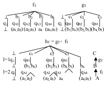
Figure 2: composed tree

Notice that the arrows (morphisms) in $DB$ are not functions. Thus, $DB$ is different from $Set$ category. In order to explain the composition of morphisms let us consider the following example:
Example 2: Let us consider the morphisms $f:A\longrightarrow B$, $g:B\longrightarrow C$, such that
$A=\{a_{1},..,a_{6}\},~{}B=\{b_{1},..,b_{7}\},~{}C=\{c_{1},..,c_{4}\},~{}where~{}f=\{q_{A_{1}},..,q_{A_{4}}\},with~{}\\ \partial_{0}(q_{A_{1}})=\{a_{1},a_{2}\},~{}\partial_{0}(q_{A_{2}})=\{a_{2},a_{3}\},~{}\partial_{0}(q_{A_{3}})=\{a_{4}\},~{}\partial_{0}(q_{A_{4}})=\{a_{4},a_{5}\},\\ ~{}\partial_{1}(q_{A_{1}})=\{b_{1}\},~{}\partial_{1}(q_{A_{2}})=\{b_{2}\},~{}\partial_{1}(q_{A_{3}})=\{b_{3}\},~{}\partial_{1}(q_{A_{4}})=\{b_{6}\},~{}~{}and~{}g=\{q_{B_{1}},..,q_{B_{3}}\},\\ with~{}\partial_{0}(q_{B_{1}})=\{b_{1},b_{4}\},~{}\partial_{0}(q_{B_{2}})=\{b_{2},b_{3}\},~{}\partial_{0}(q_{B_{3}})=\{b_{4},b_{5}\},~{}\partial_{1}(q_{B_{1}})=\{c_{1}\},~{}\partial_{1}(q_{B_{2}})=\{c_{2}\},~{}\partial_{1}(q_{B_{3}})=\{c_{3}\}$, that can be represented by trees $f_{T}=f$ and $g_{T}=g$ and their sequential composition $h_{T}$ (Fig. 2).
The composition of morphisms (Fig. 3) $h=g\circ f:A\longrightarrow C$ may be represented as a part of the tree $h_{T}$ that gives information contribution from the object $A$ (source) into the object $C$ (target of this composed morphism). We have that $\partial_{0}(f)=\{a_{1},a_{2},a_{3},a_{4},a_{5}\}$, $\partial_{1}(f)=\{b_{1},b_{2},b_{3},b_{6}\}$, $\partial_{0}(g)=\{b_{1},b_{2},b_{3},b_{4},b_{5}\}$, $\partial_{1}(g)=\{c_{1},c_{2},c_{3}\}$, while $\partial_{0}(h)=\partial_{0}(g\circ f)=\{a_{1},a_{2},a_{3},a_{4}\}\neq\partial_{0}(f),~{}~{}\partial_{1}(h)=\partial_{1}(g\circ f)=\{c_{1},c_{2}\}\neq\partial_{1}(g)$

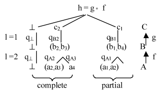
Figure 3: obtained partial morphism

Let us see, for example, the composition of the c-arrow $h:C\longrightarrow D$ with the composed arrow $g\circ f$ in the previous example, where $D=\{d_{1},..,d_{4})\}$, $h=\{q_{C_{1}},q_{C_{2}},q_{C_{3}}\}$, $~{}\partial_{0}(q_{C_{1}})=\{c_{2}\}$,$~{}\partial_{1}(q_{C_{1}})=\{d_{1}\}$, $~{}\partial_{0}(q_{C_{2}})=\{c_{1},c_{2},c_{3}\}$,$~{}\partial_{1}(q_{C_{2}})=\{d_{2}\}$, $~{}\partial_{0}(q_{C_{3}})=\{c_{1},c_{4}\}$,$~{}\partial_{1}(q_{C_{3}})=\{d_{3}\}$, with $q_{B_{2}}(tree)=q_{B_{2}}\circ\{q_{A_{2}},~{}q_{A_{3}}\}$ a complete, and $q_{B_{1}}(tree)=q_{B_{1}}\circ\{q_{A_{1}},~{}-~{}\}$ a partial (incomplete) component of this tree, as represented in the Fig. 4.

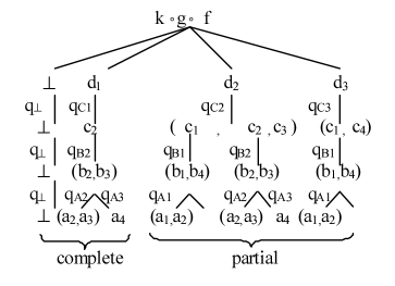
Figure 4: composed morphism

As we see, a composition of (complete) morphisms generally produces a partial (incomplete) morphism (only a part of the tree $h_{T}$ represents a real contribution from $A$ into $C$) with hidden elements (in the diagram of the composed morphism $h$, the element $b_{4}$ is a hidden element). In such a representation we ”forgot” parts of the tree $g_{T}\circ f_{T}$ that are not involved in real information contribution of composed mappings from the source into the target object. So, we define the semantics of any morphism $h:A\longrightarrow C$ as an ”information transmitted flux” from the source into the target object. An ”information flux” (denoted by $~{}\widetilde{h}$) is a set set of views (so, it is an object in $DB$ category as well) which is ”transmitted” by a mapping.
$\square$

In order to explain this concept of ”information flux” let us consider a simple morphism $f:A\longrightarrow B~{}$ from a database $A$ into a database $B$, composed by only one view map based on a single query $q(\textbf{x})\longleftarrow R_{1}(u_{1}),...,R_{n}(u_{n})$, where $n\geq 0$, $R_{i}$ are relation names (at least one) in $\mathcal{A}$ or built-in predicates (ex. $\leq,=,$ etc..), and $q$ is a relation name not in $\mathcal{A}$. Then, for any tuple c for which the body of this query is true, also $q(\textbf{c})$ must be true, that is, this tuple from a database $A$ ”is transmitted” by this view-mapping into one relation of database $B$. The set (n-ary relation) $Q$ of all tuples that satisfy the body of this query will constitute the whole information ”transmitted” by this mapping. The ”information flux” $\widetilde{f}$ of this mapping is the set $TQ$, that is, the set of all views (possible observations) that can be obtained from the transmitted information of this mapping.

Definition 7

We define the semantics of mappings by function $B_{T}:Mor_{DB}\longrightarrow Ob_{DB}$, which, given any mapping morphism $f:A\longrightarrow B~{}$, returns with the set of views (”information flux”) that are really ”transmitted” from the source to the target object.
1. For an atomic morphism, $\widetilde{f}=B_{T}(f)~{}\triangleq T\{\|q_{A_{i}}\|~{}|~{}q_{A_{i}}\in f\}$.
2. Let $g:A\rightarrow B$ be a morphism with a flux $\widetilde{g}$, and $f:B\rightarrow C$ an atomic morphism with flux $\widetilde{f}$ defined in point 1, then $~{}~{}\widetilde{f\circ g}=B_{T}(f\circ g)~{}\triangleq\widetilde{f}\bigcap\widetilde{g}$.

Thus we have the following fundamental property:

Proposition 1

Any mapping morphism $f:A\longrightarrow B~{}$ is a closed object in DB, i.e., $~{}~{}\widetilde{f}=T\widetilde{f}$.

Proof: This proposition may be proved by structural induction; each atomic arrow is a closed object ($T\widetilde{f}=T(T\{\|q_{A_{i}}\|~{}|~{}q_{A_{i}}\in f\})=T\{\|q_{A_{i}}\|~{}|~{}q_{A_{i}}\in f\}=\widetilde{f}$, each arrow is a composition of a number of complete arrows, and intersection of closed objects is always a closed object.
$\square$
Remark: The ”information flux” $\widetilde{f}$ of a given morphism (mapping) $f:A\longrightarrow B$ is an instance-database as well (its elements are the views defined by the formulae above), thus, an object in $DB$: the minimal ”information flux” is equal to the bottom object $\bot^{0}$ so that, given any two database instances $A,B$ in $DB$, there exists at least an arrow (morphism) between them $f:A\longrightarrow B$ such that $\widetilde{f}=\bot^{0}$.

Proposition 2

The following properties for morphisms are valid:

1. each arrow $f:A\twoheadrightarrow B$, such that $~{}\widetilde{f}=TB$ is an epimorphism

2. each arrow $f:A\hookrightarrow B$, such that $~{}\widetilde{f}=TA$ is a monomorphism

3. each monic and epic arrow is an isomorphism, thus two objects A and B are isomorphic iff $~{}~{}TA=TB$, i.e.,

   $$A\backsimeq B~{}~{}~{}~{}iff~{}~{}~{}~{}TA=TB$$

Proof: 1. An arrow $f:A\twoheadrightarrow B$ is epic iff for any $h,g:B\longrightarrow C$ holds $(h\circ f=g\circ f)\Rightarrow(h=g)$, thus $(\widetilde{h\circ f}=\widetilde{g\circ f})\Rightarrow(\widetilde{h}=\widetilde{g})$ which is satisfied by $\widetilde{f}=TB$ (because $\widetilde{h}\subseteq TB~{}and~{}\widetilde{g}\subseteq TB$)
2. An arrow $f:A\longrightarrow B$ is monic iff for any $h,g:C\longrightarrow A$ holds $(f\circ h=f\circ g)\Rightarrow(h=g)$, thus $(\widetilde{f\circ h}=\widetilde{f\circ g})\Rightarrow(\widetilde{h}=\widetilde{g})$ which is satisfied by $\widetilde{f}=TA$ (because $\widetilde{h}\subseteq TA~{}and~{}\widetilde{g}\subseteq TA$)
3. By 1 and 2, because an isomorphism is epic and monic, and viceversa if $f$ is monic and epic then $\widetilde{f}=TA$ (2) and $\widetilde{f}=TB$ (1), thus $TA=TB$. It is enough to show the isomorphism $A\backsimeq TA$ : let us define the isomorphisms $is_{A}:A\longrightarrow TA$, and its inverse $is^{-1}_{A}:TA\longrightarrow A$,

$$\ is_{A}=\bigcup_{\partial_{1}(q_{A_{i}})=\{v\}~{}\&~{}v\in TA}~{}\{q_{A_{i}}\},~{}~{}~{}~{}is^{-1}_{A}=\bigcup_{\partial_{0}(q_{TA_{i}})=\partial_{1}(q_{TA_{i}})~{}\&~{}\partial_{1}(q_{TA_{i}})=\{v\}~{}\&~{}v\in A}~{}\{q_{TA_{i}}\}$$

Thus, $\widetilde{is_{A}}=\widetilde{is^{-1}_{A}}=TA$, so it holds that $\widetilde{is^{-1}_{A}\circ is_{A}}=TA=\widetilde{id_{A}}=\widetilde{is_{A}\circ is^{-1}_{A}}$, i.e., $is^{-1}_{A}\circ is_{A}=id_{A}$ and $is_{A}\circ is^{-1}_{A}=id_{TA}$, thus $A\backsimeq TA$. Finally, $~{}~{}A\backsimeq TA=TB\backsimeq B$, i.e.,$~{}~{}A\backsimeq B$.
$\square$
Remark: Thus, we consider, for example, the real object (empty database instance) $\bot^{0}$ as zero object (both terminal and initial) in $DB$, (from any real object $A$ in $DB$ there is a unique arrow from it into $\bot^{0}$ and its reversed arrow). Each arrow $f$ with $\partial_{0}(f)=\{\bot\}$ or $\partial_{1}(f)=\bot$ has an empty flux, thus does not give any information contribution to the target database: as for example Yes arrows in $DB$ for Yes/No queries.
It is easy to verify that each empty database (with all empty relations) is isomorphic to the zero object $\bot^{0}$.
In what follows we will show that any two isomorphic objects (databases) in $DB$ are observationally equivalent.

3.1 Interpretations of schema mappings

The semantics of mapping between two relational database schemas, $f:\mathcal{A}\longrightarrow\mathcal{B}$, is a constraint on the pairs of interpretations, of $\mathcal{A}$ and $\mathcal{B}$, and therefore specifies which pairs of interpretations can co-exist, given the mapping (see also  [1]). We consider only view-based mappings between schemas defined in the SQL language of $SPJRU$ algebra, i.e., when
$(1)~{}~{}~{}f=\{q_{Ai}(x)\Rightarrow b_{j}(x)\}$, where $q_{Ai}(x)$ is a union of conjunctive queries over $\mathcal{A}$ and $b_{j}$ is a relation symbol of a database schema $\mathcal{B}$, or,
$(2)~{}~{}~{}f=\{q_{Ai}(x)\Rightarrow q_{Bj}(x)\}$, where $q_{Bj}(x)$ is a union of conjunctive queries over $\mathcal{B}$. In this case the mapping $f$ also involves a helper database schema $\mathcal{C}$ with a relation $c_{i}(x)$ for each $q_{Ai}(x)\in f$ with two new database mappings, $f_{AC}:\mathcal{A}\rightarrow\mathcal{C}$ and $f_{BC}:\mathcal{B}\rightarrow\mathcal{C}$, with $f_{AC}=\{q_{Ai}(x)\Rightarrow c_{i}(x)\}$ and $f_{BC}=\{q_{Bj}(x)\Rightarrow c_{i}(x)\}$.
The formula $e=~{}q_{Ai}(x)\Rightarrow q_{Bj}(x)$ (logical implication between queries), means that each tuple of the view obtained by the query $q_{Ai}(x)$ is also a tuple of the view obtained by the query $q_{Bj}(x)$.
There is a fundamental functorial interpretation connection from schema mappings and their models in the instance level category $DB$: based on the Lawvere categorial theories [22, 23], where he introduced a way of describing algebraic structures using categories for theories, functors (into base category $Set$, which we will substitute by more adequate category $DB$), and natural transformations for morphisms between models. For example, Lawvere’s seminal observation that the theory of groups is a category with group object, that group in $Set$ is a product preserving functor, and that a morphism of groups is a natural transformation of functors, is an original new idea that was successively extended in order to define the categorial semantics for different algebraic and logic theories. This work is based on the theory of sketches, which are fundamentally graphs enriched by other concepts such as (co)cones mapped by functors in (co)limits of the base category $Set$. It was demonstrated that, for every sentence in basic logic, there is a sketch with the same category of models, and vice versa [24]. Accordingly, sketches are called graph-based logic and provide very clear and intuitive specification of computational data and activities. For any small sketch $E$ the category of models $Mod(E)$ is an accessible category by Lair’s theorem and reflexive subcategory of $Set^{E}$ by Ehresmann-Kennison theorem. In what follows we will substitute the base category $Set$ by this new database category $DB$.

Proposition 3

Let $Sch(G)~{}$ be a schema category generated from a schema mapping graph (sketch) $G$ . Every interpretation R-algebra $\alpha~{}$ has as its categorial correspondent the functor (categorial model) $~{}\alpha^{*}:Sch(G)\longrightarrow DB~{}$, defined as follows:

1. for any database schema $\mathcal{A}=\{a_{1},...,a_{n}\}$, (object in $Sch(G)$), where $a_{i}\in R,~{}i=1,..,n$, holds $A\triangleq\alpha^{*}(\mathcal{A})=\{\alpha(a_{1}),...,\alpha(a_{n})\}$, i.e., $A$ is an interpretation (logical model) of a database schema $\mathcal{A}$.

2. for any schema mapping arrow $f:\mathcal{A}\longrightarrow\mathcal{B}$, let $~{}~{}f_{T}~{}~{}$ be the tree structure of operads, $f_{T}=\{f_{1}\cdot g_{1},...,f_{k}\cdot g_{k})\}$, where each $f_{i}$ is a linear composition of operads, then $\alpha^{*}(f)=\{\alpha(f_{1})\circ\alpha^{*}(g_{1}),...,\alpha(f_{k})\circ\alpha^{*}(g_{k})\}$, otherwise $\alpha^{*}(f)=\alpha(f_{T})$.
   Formally, the satisfaction of mapping $f$ is defined as follows: for each logical formula $~{}~{}e\in f$, $~{}~{}~{}\{\alpha^{*}(\mathcal{A}),\alpha^{*}(\mathcal{B})\}\vDash~{}e$, that is $e$ is satisfied by a model $\alpha^{*}\in Mod(Sch(G))\subseteq DB^{Sch(G)}$.

Proof: This is easy to verify, based on general theory for sketches [23]: each arrow in a sketch (enriched schema mapping graph) $G$ may be converted into a tree syntax structure of some morphism in $DB$ (labeled tree without any interpretation), thus, a sketch $G$ can be extended into a category $Sch(G)$. (The composition of schema mappings in the category $Sch(G)$, where each mapping is a set of first-order logical formulas, can be defined as a disjoint union). The functor is only the simple extension of the interpretation R-algebra function $\alpha~{}$ for a lists of symbols, as in Definition 5.
$\square$

3.2 Power-view endofunctor T

Let us extend the notion of the type operator $T$ into a notion of the endofunctor in $DB$ category:

Theorem 1

There exists an endofunctor $T=(T^{0},T^{1}):DB\longrightarrow DB$, such that

1. for any object A, the object component $T^{0}$ is equal to the type operator T, i.e., $~{}~{}~{}~{}T^{0}(A)\triangleq TA$

2. for any morphism $~{}f:A\longrightarrow B$, the arrow component $T^{1}$ is defined by

   $$\ T(f)\triangleq T^{1}(f)=\bigcup_{\partial_{0}(q_{TA_{i}})=\partial_{1}(q_{TA_{i}})=\{v\}~{}\&~{}v\in~{}\widetilde{f}}\{q_{TA_{i}}:TA\rightarrow TB\}$$

3. Endofunctor T preserves the properties of arrows, i.e., if a morphism $f$ has a property P (monic, epic, isomorphic), then also $T(f)$ has the same property: let $P_{mono},P_{epi}~{}and~{}\\ P_{iso}$ are monomorphic, epimorphic and isomorphic properties respectively, then the following formula is true
   $\forall(f\in Mor_{DB})(P_{mono}(f)\equiv P_{mono}(Tf)$ and $P_{epi}(f)\equiv P_{epi}(Tf)$ and $P_{iso}(f)\equiv P_{iso}(Tf)$.

Proof: It is easy to verify that $T$ is a 2-endofunctor and to see that $T$ preserves properties of arrows: for example, if $P_{mono}(f)$ is true for an arrow $f:A\longrightarrow B$, then $\widetilde{f}=TA$ and $\widetilde{Tf}=T\widetilde{f}=T(TA)=TA$, thus $P_{mono}(Tf)$ is true. Viceversa, if $P_{mono}(Tf)$ is true then $\widetilde{Tf}=T\widetilde{f}=T(TA)$, i.e., $\widetilde{f}=TA$ and, consequently, $P_{mono}(f)$ is true.
$\square$
The endofunctor $T$ is a right and left adjoint to identity functor $I_{DB}$, i.e., $T\simeq I_{DB}$. Thus we have the equivalence adjunction $<T,I_{DB},\eta^{C},\eta>$ with the unit $\eta^{C}:T\simeq I_{DB}$ (such that for any object $A$ the arrow $\eta^{C}_{A}\triangleq\eta^{C}(A)\equiv is^{-1}_{A}:TA\longrightarrow A$), and the counit $\eta:I_{DB}\simeq T$ (such that for any $A$ the arrow $\eta_{A}\triangleq\eta(A)\equiv is_{A}:A\longrightarrow TA$) are isomorphic arrows in $DB$ (by duality theorem it holds that $\eta^{C}=\eta^{inv}$).
The function $T^{1}:(A\longrightarrow B)\longrightarrow(TA\longrightarrow TB)~{}$ is not a higher-order function (arrows in $DB$ are not functions): thus, there is no correspondent monad-comprehension for the monad $T$, which invalidates the thesis  [25] that ”monads $\equiv~{}$ monad-comprehensions”. It is only valid that ”monad-comprehensions $\Rightarrow~{}$ monads”.
We have already seen that the views of a database can be seen as its observable computations: what we need, to obtain an expressive power of computations in the category $DB$, are the categorial computational properties, as known, based on monads:

Proposition 4

The power-view closure 2-endofunctor $T=(T^{0},T^{1}):DB\longrightarrow DB~{}$ defines the monad $(T,\eta,\mu)~{}$ and the comonad $(T,\eta^{C},\mu^{C})~{}$ in DB, such that $\eta:I_{DB}\backsimeq T~{}$ and $\eta^{C}:T\backsimeq I_{DB}~{}$ are natural isomorphisms, while $\mu:TT\longrightarrow T~{}$ and $\mu^{C}:T\longrightarrow TT~{}$ are equal to the natural identity transformation $id_{T}:T\longrightarrow T~{}$ (because T = TT).

Proof: It is easy to verify that all commutative diagrams of the monad ($\mu_{A}\circ\mu_{TA}=\mu_{A}\circ T\mu_{A}~{}$, $\mu_{A}\circ\eta_{TA}=id_{TA}=\mu_{A}\circ T\eta_{A}$) and the comonad are diagrams composed by identity arrows. Notice that by duality we obtain $\eta_{TA}=T\eta_{A}=\mu^{inv}_{A}$.
$\square$

3.3 Duality

The following duality theorem tells us that, for any commutative diagram in $DB$, there is the same commutative diagram composed by equal objects and by inverted equivalent arrows as well. This ”bidirectional” mappings property of $DB$ is a consequence of the fact that a composition of arrows is semantically based on the set-intersection commutativity property for ”information fluxes” of its arrows. Thus any limit diagram in $DB$ also has its ”reversed” equivalent colimit diagram with equal objects, and any universal property also has its equivalent couniversal property in $DB$.

Theorem 2

there exists the controvariant functor $\underline{S}=(\underline{S}^{0},\underline{S}^{1}):DB\longrightarrow DB$ such that

1. $\underline{S}^{0}$ is an identity function on objects.

2. for any arrow in $DB$, $f:A\longrightarrow B$ we have $\underline{S}^{1}(f):B\longrightarrow A$, such that $\underline{S}^{1}(f)\triangleq f^{inv}$, where $f^{inv}$ is an (equivalent) reversed morphism of $~{}f~{}~{}~{}$ (i.e., $\widetilde{f^{inv}}=\widetilde{f}$),
   $f^{inv}=is^{-1}_{A}\circ(Tf)^{inv}\circ is_{B}~{}$ with

   $$\ (Tf)^{inv}~{}\triangleq\bigcup_{\partial_{0}(q_{TB_{j}})=\partial_{1}(q_{TB_{j}})=\{v\}~{}\&~{}v\in~{}\widetilde{f}}\{q_{TB_{j}}:TB\rightarrow TA\}$$

3. The category DB is equal to its dual category $DB^{OP}$.

Proof: We have, from the definition of reversed arrow, that, $\widetilde{f^{inv}}=\widetilde{is^{-1}_{A}}\bigcap\widetilde{(Tf)^{inv}}\bigcap\widetilde{is_{B}}\\ =TA\bigcap\widetilde{(Tf)^{inv}}\bigcap TB=TA\bigcap\widetilde{Tf}\bigcap TB=TA\bigcap\widetilde{f}\bigcap TB=\widetilde{f}$. The reversed arrow of any identity arrow is equal to it, and, also, the compositional property for functor holds (the intersection operator for ”information fluxes” is commutative). Thus, the controvariant functor is well defined.
It is convenient to represent this controvariant functor as a covariant functor $S:DB^{OP}\\ \longrightarrow DB$, or a covariant functor $S^{OP}:DB\longrightarrow DB^{OP}$. It is easy to verify that for compositions of these covariant functors hold, $SS^{OP}=I_{DB}$ and $S^{OP}S=I_{DB^{OP}}$ w.r.t. the adjunction $<S,S^{OP},\phi>:DB^{OP}\longrightarrow DB$, where $\phi~{}$ is a bijection: for each pair of objects $A,B$ in $DB$ we have the bijection of hom-sets, $\phi_{A,B}:DB(A,S(B))\simeq DB^{OP}(S^{OP}(A),B)$, i.e., $\phi_{A,B}:DB(A,B)\simeq DB(B,A)$, such that for any arrow $f\in DB(A,B)~{}$ holds $\phi_{A,B}(f)=S^{1}(f)=f^{inv}$. The unit and counit of this adjunction are the identity natural transformations, $\eta_{OP}:I_{DB}\longrightarrow SS^{OP}$, $\epsilon_{OP}:S^{OP}S\longrightarrow I_{DB^{OP}}~{}$ respectively, such that for any object $A$ they return by its identity arrow. Thus, from this adjunction, we obtain that $DB$ is isomorphic to its dual $DB^{OP}$; moreover they are equal because they have the same objects and the same arrows.
$\square$
Let us introduce the concepts for products and coproducts in $DB$ category.

Definition 8

The disjoint union of any two instance-databases (objects) A and B, denoted by $~{}A+B$, corresponds to two mutually isolated databases, where two database management systems are completely disjoint, so that it is impossible to compute the queries with the relations from both databases.
The disjoint property for mappings is represented by facts that
$\partial_{0}(f+g)\triangleq\partial_{0}(f)+\partial_{0}(g),~{}~{}~{}\partial_{1}(f+g)\triangleq\partial_{1}(f)+\partial_{1}(g)$.

Thus, for any database $A$, the replication of this database (over different DB servers) can be denoted by the coproduct object $A+A$ in this category $DB$.

Proposition 5

For any two databases (objects) A and B we have that $T(A+B)=TA+TB$. Consequently $A+A$ is not isomorphic to $A$.

Proof: We have that $T(A+B)=TA+TB$, directly from the fact that we are able to define views only over relations in $A$ or, alternatively, over relations in $B$. Analogously $~{}~{}\widetilde{f+g}=\widetilde{f}+\widetilde{g}$, which is a closed object, that is, holds that $T(\widetilde{f+g})=T(\widetilde{f}+\widetilde{g})=T\widetilde{f}+T\widetilde{g}=\widetilde{f}+\widetilde{g}=\widetilde{f+g}$.
From $T(A+A)=TA+TA\neq TA$ we obtain that $A+A$ is not isomorphic to $A$.
$\square$
Notice that for coproducts holds that $~{}~{}C+\perp^{0}~{}=~{}\perp^{0}+C~{}\simeq~{}C$, and for any arrow $f$ in $DB$, $~{}~{}f+\perp^{1}~{}\approx~{}\perp^{1}+f~{}\approx~{}f$, where $~{}\perp^{1}~{}$ is a banal empty morphism between objects, such that $~{}\partial_{0}(\perp^{1})=\partial_{1}(\perp^{1})=\perp^{0}$, with $\widetilde{\perp^{1}}=\perp^{0}$.
We are ready now to introduce the duality property between coproducts and products in this $DB$ category:

Proposition 6

There exists an idempotent coproduct bifunctor $+:DB\times DB\longrightarrow DB$ which is a disjoint union operator for objects and arrows in DB.
The category DB is cocartesian with initial (zero) object $~{}\perp^{0}$ and for every pair of objects A,B it has a categorial coproduct $A+B$ with monomorphisms (injections) $in_{A}:A\hookrightarrow A+B~{}$ and $in_{B}:B\hookrightarrow A+B$.
By duality property we have that DB is also cartesian category with a zero object $~{}\perp^{0}$. For each pair of objects A,B there exists a categorial product $A\times B$ with epimorphisms (projections) $p_{A}=in^{inv}_{A}:A\times A\twoheadrightarrow A~{}$ and $p_{B}=in^{inv}_{B}:B\times B\twoheadrightarrow B$, where the product bifunctor is equal to the coproduct bifunctor, i.e., $\times~{}\equiv~{}+$.

Proof: 1. For any identity arrow $(id_{A},id_{B})$ in $DB\times DB$, where $id_{A},~{}id_{b}~{}$ are the identity arrows of $A$ and $B$ respectively, holds that $\widetilde{id_{A}+id_{B}}=\widetilde{id_{A}}+\widetilde{id_{B}}=TA+TB=T(A+B)=\widetilde{id_{A+B}}$. Thus, $+^{1}(id_{A},id_{B})=id_{A}+id_{B}=id_{A+B}$, is an identity arrow of the object $A+B$.
2. For any given $k:A\longrightarrow A_{1}$, $~{}k_{1}:A_{1}\longrightarrow A_{2}$, $~{}l:B\longrightarrow B_{1}$, $~{}l_{1}:B_{1}\longrightarrow B_{2}$, holds $\widetilde{+^{1}(k_{1},l_{1})\circ+^{1}(k,l)}=\widetilde{+^{1}(k_{1},l_{1})}\bigcap\widetilde{+^{1}(k,l)}=\widetilde{k_{1}\circ k+l_{1}\circ l}=\widetilde{+^{1}(k_{1}\circ k,~{}l_{1}\circ l)}\\ =\widetilde{+^{1}((k_{1},k)\circ(l_{1},l))}$, thus $~{}+^{1}(k_{1},l_{1})\circ+^{1}(k,l)=+^{1}((k_{1},k)\circ(l_{1},l)).$
3. Let us demonstrate the coproduct property of this bifunctor: for any two arrows $f:A\longrightarrow C$, $g:B\longrightarrow C$, there exists a unique arrow $k:A+B\longrightarrow C$, such that $f=k\circ in_{A}$, $g=k\circ in_{B}$, where $in_{A}:A\hookrightarrow A+B$, $in_{B}:B\hookrightarrow A+B~{}$ are the injection (point to point) monomorphisms ($\widetilde{in_{A}}=TA,~{}\widetilde{in_{B}}=TB$).
It is easy to verify that for any two arrows $f:A\longrightarrow C$, $g:B\longrightarrow C$, there is exactly one arrow $k=e_{C}\circ(f+g):A+B\longrightarrow C$, where $e_{C}:C+C\twoheadrightarrow C$ is an epimorphism (with $\widetilde{e_{C}}=TC$), such that $\widetilde{k}=\widetilde{f}+\widetilde{g}$.
$\square$
The following proposition introduces the pullbacks (and pushouts, by duality) for the category $DB$.

Proposition 7

For any given pair of arrows with the same codomain, $f:A\longrightarrow C$ and $g:B\longrightarrow C$, there is a pullback with the fibred product $D=\widetilde{f}\bigcap\widetilde{g}$ (product of A and B over C). By duality, for any pair of arrows with the same domain there is a pushout as well.
DB is a complete and cocomplete category.

Proof: We define the commutative diagram $f\circ h_{A}=h_{B}\circ g$, where $h_{A}:D\hookrightarrow A$ and $h_{B}:D\hookrightarrow B$ are monomorphisms defined by $h_{A}=is^{-1}_{A}\circ in_{DA}$, $h_{B}=is^{-1}_{B}\circ in_{DB}$, where $is^{-1}_{A}:TA\longrightarrow A$, $~{}is^{-1}_{B}:TB\longrightarrow B$ are isomorphisms and $~{}in_{DA}:D\hookrightarrow TA$, $~{}in_{DB}:D\hookrightarrow TB~{}$ are monomorphisms, such that $\widetilde{h_{A}}=\widetilde{h_{B}}=\widetilde{f}\bigcap\widetilde{g}=D$.
Let us show that for any pair of arrows $l_{A}:E\longrightarrow A$, $l_{B}:E\longrightarrow B$, such that $f\circ l_{A}=l_{B}\circ g$ there is a unique arrow $k:E\longrightarrow D$ such that a pullback diagram commutes, i.e., (a) that $l_{A}=h_{A}\circ k~{}$ and $l_{B}=h_{B}\circ k$. In fact, it must hold $\widetilde{k}\subseteq TD=T(\widetilde{f}\bigcap\widetilde{g})=\widetilde{f}\bigcap\widetilde{g}=\widetilde{h_{A}}=\widetilde{h_{B}}$. So, from the commutativity (a), $\widetilde{l_{A}}=\widetilde{h_{A}}\bigcap\widetilde{k}=\widetilde{k}~{}$ and $\widetilde{l_{B}}=\widetilde{h_{B}}\bigcap\widetilde{k}=\widetilde{k}$. Thus , for any other arrow $k_{1}:E\longrightarrow D$ that makes a commutativity (a) must hold that $\widetilde{k_{1}}=\widetilde{l_{A}}=\widetilde{l_{B}}$ and, consequently, $\widetilde{k_{1}}=\widetilde{k}$, i.e., $k_{1}=k$.
Consequently, $DB$ is a cartesian category with a terminal object and pullbacks, thus it is complete (has all limits). By duality we deduce that it is also cocomplete (has all colimits).
$\square$
In order to explain these concepts in another way, we can see the limits and colimits as a left and a right adjunction for the diagonal functor $\bigtriangleup:DB\longrightarrow DB^{J}$ for any small index category (i.e., a diagram) $J$. For any colimit functor $F:DB^{J}\longrightarrow DB$ we have a left adjunction to diagonal functor $<F,\bigtriangleup,\eta_{C},\varepsilon_{C}>:DB^{J}\longrightarrow DB$, with the colimit object $F(D)$ for any object (diagram) $D\in DB^{J}$ and the universal cone, a natural transformation, $\eta_{C}:Id_{DB^{J}}\longrightarrow\bigtriangleup F$. Then, by duality, the same functor $F$ is also a right adjoint to the diagonal functor (adjunction, $<\bigtriangleup,F,\eta,\varepsilon>:DB\longrightarrow DB^{J}$), with the limit object (equal to the colimit object above) $F(D)$ and the universal cone (counit), a natural transformation, $\varepsilon:\bigtriangleup F\longrightarrow Id_{DB^{J}}$, such that $\varepsilon=\eta^{inv}_{C}$ and $\eta=\varepsilon^{inv}_{C}$.
Let us see, for example, the coproducts ($F=+$) and products ($F=\times\equiv+$). In that case the diagram $D\in DB^{J}$ is just a diagram of two arrows with the same codomain. We obtain for the universal cone unit $\eta_{C}(<A,B>):<A,B>\longrightarrow<A+B,A+B>$ one pair of coproduct inclusion-monomorphisms $\eta_{C}(<A,B>)=<in_{A},in_{B}>$, where $in_{A}:A\hookrightarrow A+B$, $in_{B}:B\hookrightarrow A+B$. The universal cone counit of product $\varepsilon(<A\times B,A\times B>):<A\times B,A\times B>\longrightarrow<A,B>$ is a pair of product projection-epimorphisms $\varepsilon(<A\times B,A\times B>)=<p_{A},p_{B}>$, where $p_{A}:A\times B\twoheadrightarrow A$, $p_{B}:A\times B\twoheadrightarrow B$, $A\times B=A+B$, $p_{A}=in^{inv}_{A}$, $p_{B}=in^{inv}_{B}$, as represented in the following diagram: Example 3: Let us verify that each object in $DB$ is a limit of some equalizer and a colimit of its dual coequalizer. In fact, for any object $A$, a ”structure map” $h:TA\longrightarrow A$ of a monadic T-algebra $<A,h>$ derived from a monad $(T,\eta,\mu)$ (where $h\circ\eta_{A}=id_{A}$, so that $h$ is an isomorphism $h=\eta^{inv}_{A}=\eta^{C}_{A}$, i.e., $\widetilde{h}=TA=\widetilde{id_{A}}$) we obtain the absolute coequalizer (by Back’s theorem, it is preserved by the endofunctor $T$, i.e., $T$ creates a coequalizer) with a colimit $A$, and, by duality, we obtain the absolute equalizer with the limit $A$ as well. $\square$

4 Equivalence relations for databases

We can introduce a number of different equivalence relations for instance-databases:

• Identity relation: Two instance-databases (sets of relations) $A$ and $B$ are identical when holds the set identity $A=B$.

• behavioral equivalence relation: Two instance-databases $A$ and $B$ are behaviorally equivalent when each view obtained from a database $A$ can also be obtained from a database $B$ and viceversa.

• weak observational equivalence relation: Two instance-databases $A$ and $B$ are weakly equivalent when each ”certain” view (without Skolem constants) obtained from a database $A$ can be also obtained from a database $B$ and viceversa.

It is also possible to define other kinds of equivalences for databases. In the rest of this chapter we will consider only the second and third equivalences defined above.

4.1 The (strong) behavioral equivalence for databases

Let us now consider the problem of how to define equivalent (categorically isomorphic) objects (database instances) from a behavioral point of view based on observations: as we see, each arrow (morphism) is composed by a number of ”queries” (view-maps), and each query may be seen as an observation over some database instance (object of $DB$). Thus, we can characterize each object in $DB$ (a database instance) by its behavior according to a given set of observations. Indeed, if one object $A$ is considered as a black-box, the object $TA$ is only the set of all observations on $A$. So, given two objects $A$ and $B$, we are able to define the relation of equivalence between them based on the notion of the bisimulation relation. If the observations (resulting views of queries) of $A$ and $B$ are always equal, independent of their particular internal structure, then they look equivalent to an observer.
In fact, any database can be seen as a system with a number of internal states that can be observed by using query operators (i.e, programs without side-effects). Thus, databases $A$ and $B$ are equivalent (bisimilar) if they have the same set of observations, i.e. when $TA$ is equal to $TB$:

Definition 9

The relation of (strong) behavioral equivalence ${}^{\prime}\approx^{\prime}$ between objects (databases) in $DB$ is defined by

$$\ A\approx B~{}~{}iff~{}~{}TA=TB$$

the equivalence relation for morphisms is given by,

$$f\approx g~{}~{}~{}~{}iff~{}~{}~{}~{}\widetilde{f}=\widetilde{g}$$

This relation of behavioral equivalence between objects corresponds to the notion of isomorphism in the category $DB$ (see Proposition 2).
This introduced equivalence relation for arrows $\approx$, may be given by an (interpretation) function $B_{T}:Mor_{DB}\longrightarrow Ob_{DB}~{}$ (see Definition 7), such that $\approx$ is equal to the kernel of $B_{T}$, ($\approx~{}=~{}kerB_{T}$), i.e., this is a fundamental concept for categorial symmetry  [26]:

Definition 10

Categorial symmetry:
Let C be a category with an equivalence relation $~{}\approx~{}\subseteq Mor_{C}\times Mor_{C}$ for its arrows (equivalence relation for objects is the isomorphism $~{}\backsimeq~{}\subseteq Ob_{C}\times Ob_{C}$) such that there exists a bijection between equivalence classes of $\approx$ and $\backsimeq$, so that it is possible to define a skeletal category $|C|$ whose objects are defined by the imagine of a function $B_{T}:Mor_{C}\longrightarrow Ob_{C}$ with the kernel $~{}kerB_{T}=~{}\thickapprox$, and to define an associative composition operator for objects $*$, for any fitted pair $g\circ f$ of arrows, by $~{}~{}B_{T}(g)*B_{T}(f)=B_{T}(g\circ f)$.
For any arrow in C, $f:A\longrightarrow B$, the object $B_{T}(f)$ in C, denoted by $~{}\widetilde{f}$, is denominated as a conceptualized object.

Remark: This symmetry property allows us to consider all the properties of an arrow (up to the equivalence) as properties of objects and their composition as well. Notice that any two arrows are equal if and only if they are equivalent and have the same source and the target objects.
We have that in symmetric categories holds that $f\approx g$ iff $\widetilde{f}\simeq\widetilde{g}$.
Let us introduce, for a category $C$ and its arrow category $C\downarrow C$, an encapsulation operator $J:Mor_{C}\longrightarrow Ob_{C\downarrow C}$, that is, a one-to-one function such that for any arrow $f:A\longrightarrow B$, $J(f)=<A,B,f>$ is its correspondent object in $C\downarrow C$, with its inverse $~{}\psi~{}$ such that $\psi(<A,B,f>)=f$.
We denote by $F_{st},S_{nd}:(C\downarrow C)\longrightarrow C~{}$ the first and the second comma functorial projections (for any functor $F:C\rightarrow D$ between categories $C$ and $D$, we denote by $F^{0}$ and $F^{1}$ its object and arrow component), such that for any arrow $(k_{1};k_{2}):<A,B,f>\rightarrow<A^{\prime},B^{\prime},g>$ in $C\downarrow C$ (such that $k_{2}\circ f=g\circ k_{1}$ in $C$), we have that $F_{st}^{0}(<A,B,f>)=A,F_{st}^{1}(k_{1};k_{2})=k_{1}$ and $S_{nd}^{0}(<A,B,f>)=B,S_{nd}^{1}(k_{1};k_{2})=k_{2}$.
We denote by $\blacktriangle:C\longrightarrow(C\downarrow C)~{}$ the diagonal functor, such that for any object $A$ in a category $C$, $\blacktriangle^{0}(A)=<A,A,id_{A}>$.
An important subset of symmetric categories are Conceptually Closed and Extended symmetric categories, as follows:

Definition 11

Conceptually closed category is a symmetric category C with a functor $T_{e}=(T_{e}^{0},T_{e}^{1}):(C\downarrow C)\longrightarrow C$ such that $T_{e}^{0}=B_{T}\psi$, i.e., $B_{T}=T_{e}^{0}J$, with a natural isomorphism $~{}\varphi:T_{e}\circ\blacktriangle~{}\backsimeq~{}I_{C}$, where $I_{C}$ is an identity functor for $C$.
C is an extended symmetric category if holds also $~{}~{}~{}\tau^{-1}\bullet\tau=\psi$, for vertical composition of natural transformations $\tau:F_{st}\longrightarrow T_{e}~{}$ and $\tau^{-1}:T_{e}\longrightarrow S_{nd}$.

Remark: it is easy to verify that in conceptually closed categories, it holds that any arrow $f$ is equivalent to an identity arrow, that is, $f\approx id_{\widetilde{f}}$.
It is easy to verify also that in extended symmetric categories the following holds:
$~{}~{}\tau=(T_{e}^{1}(\tau_{I}F_{st}^{0};\psi))\bullet(\varphi^{-1}F_{st}^{0}),~{}~{}\tau^{-1}=(\varphi^{-1}S_{nd}^{0})\bullet(T_{e}^{1}(\psi;\tau_{I}S_{nd}^{0}))$,
where $\tau_{I}:I_{C}\longrightarrow I_{C}~{}$ is an identity natural transformation (for any object $A$ in $C$, $\tau_{I}(A)=id_{A}$).
Example 4: The $Set$ is an extended symmetric category: given any function $~{}f:A\longrightarrow B$ , the conceptualized object of this function is the graph of this function (which is a set), $\widetilde{f}=B_{T}(f)=\{(x,f(x))~{}|~{}x\in A\}$.
The equivalence $\approx$ on morphisms (arrows) is defined by: two arrows $f$ and $g$ are equivalent, $f\approx g$, iff they have the same graph.
The composition of objects $*$ is defined as associative composition of binary relations (graphs), $B_{T}(g\circ f)=\{(x,(g\circ f)(x))~{}|~{}x\in A\}=\{(y,g(y))~{}|~{}y\in B\}\circ\{(x,f(x))~{}|~{}x\in A\}=B_{T}(g)*B_{T}(f)$.
$Set$ is also conceptually closed by the functor $T_{e}$, such that for any object $J(f)=<A,B,f>$, $T_{e}^{0}(J(f))=B_{T}(f)=\{(x,f(x))~{}|~{}x\in A\}$, and for any arrow $(k_{1};k_{2}):J(f)\rightarrow J(g)$, the component $T_{e}^{1}$ is defined by:
for any $(x,f(x))\in T_{e}^{0}(J(f)),~{}~{}T_{e}^{1}(k_{1};k_{2})(x,f(x))=(k_{1}(x),k_{2}(f(x)))$.
It is easy to verify the compositional property for $T_{e}^{1}$, and that $T_{e}^{1}(id_{A};id_{B})=id_{T_{e}^{0}(J(f))}$. For example, $Set$ is also an extended symmetric category, such that for any object $J(f)=<A,B,f>$ in $Set\downarrow Set$, we have that $\tau(J(f)):A\twoheadrightarrow B_{T}(f)$ is an epimorphism, such that for any $x\in A$, $~{}~{}\tau(J(f))(x)=(x,f(x))$, while $\tau^{-1}(J(f)):B_{T}(f)\hookrightarrow B$ is a monomorphism such that for any $(x,f(x))\in B_{T}(f),\\ ~{}~{}\tau^{-1}(J(f))(x,f(x))=f(x)$.
Thus, each arrow in $Set$ is a composition of an epimorphism and a monomorphism.
$\square$
Now we are ready to present a formal definition for the $DB$ category:

Theorem 3

The category DB is an extended symmetric category, closed by the functor $T_{e}=(T_{e}^{0},T_{e}^{1}):(C\downarrow C)\longrightarrow C$, where $T_{e}^{0}=B_{T}\psi~{}$ is the object component of this functor such that for any arrow $f$ in DB, $T_{e}^{0}(J(f))=\widetilde{f}$, while its arrow component $~{}T_{e}^{1}$ is defined as follows: for any arrow $(h_{1};h_{2}):J(f)\longrightarrow J(g)~{}$ in $DB\downarrow DB$, such that $g\circ h_{1}=h_{2}\circ f~{}$ in DB, holds

$$\ T_{e}^{1}(h_{1};h_{2})=\bigcup_{\partial_{0}(q_{\widetilde{f}_{i}})=\partial_{1}(q_{\widetilde{f}_{i}})=\{v\}~{}\&~{}v\in~{}\widetilde{h_{2}\circ f}}\{q_{\widetilde{f}_{i}}\}$$

The associative composition operator for objects $*$, defined for any fitted pair $g\circ f$ of arrows, is the set intersection operator $\bigcap$.
Thus, $~{}~{}B_{T}(g)*B_{T}(f)=\widetilde{g}\bigcap\widetilde{f}=\widetilde{g\circ f}=B_{T}(g\circ f)$.

Proof: Each object $A$ has its identity (point-to-point) morphism $id_{A}=\\ \bigcup_{\partial_{0}(q_{A_{i}})=\partial_{1}(q_{A_{i}})=\{v\}~{}\&~{}v\in A}\{q_{A_{i}}\}$ and holds the associativity $\widetilde{h\circ(g\circ f)}=\widetilde{h}~{}\bigcap~{}\widetilde{(g\circ f)}\\ =\widetilde{h}~{}\bigcap~{}\widetilde{g}~{}\bigcap~{}\widetilde{f}=\widetilde{(h\circ g)}~{}\bigcap~{}\widetilde{f}=\widetilde{(h\circ g)\circ f}$. They have the same source and target object, thus $h\circ(g\circ f)=(h\circ g)\circ f$. Thus, $DB$ is a category. It is easy to verify that also $T_{e}~{}$ is a well defined functor. In fact, for any identity arrow $(id_{A};id_{B}):J(f)\longrightarrow J(f)$ it holds that $T_{e}^{1}(id_{A};id_{B})=\bigcup_{\partial_{0}(q_{\widetilde{f}_{i}})=\partial_{1}(q_{\widetilde{f}_{i}})=\{v\}~{}\&~{}v\in~{}\widetilde{id_{B}\circ f}}\{q_{\widetilde{f}_{i}}\}=id_{\widetilde{f}}$ is the identity arrow of $\widetilde{f}$. For any two arrows $(h_{1};h_{2}):J(f)\longrightarrow J(g)$, $(l_{1};l_{2}):J(g)\longrightarrow J(k)$, it holds that $\overline{T_{e}^{1}(h_{1};h_{2})\circ T_{e}^{1}(l_{1};l_{2})}=\widetilde{T_{e}^{1}(h_{1};h_{2})}\bigcap\widetilde{T_{e}^{1}(l_{1};l_{2})}=T(\widetilde{l_{2}\circ g})\bigcap T(\widetilde{h_{2}\circ f})=\widetilde{l_{2}}\bigcap\widetilde{g}\bigcap\widetilde{h_{2}}\bigcap\widetilde{f}=(by~{}l_{2}\circ f=g\circ h_{1})=\widetilde{l_{2}}\bigcap\widetilde{g}\bigcap\widetilde{h_{1}}\bigcap\widetilde{h_{2}}\bigcap\widetilde{f}=(by~{}l_{2}\circ f=g\circ h_{1})=\widetilde{l_{2}}\bigcap\widetilde{h_{2}}\bigcap\widetilde{f}=\widetilde{l_{2}\circ h_{2}\circ f}=T_{e}^{1}(l_{1}\circ h_{1};l_{2}\circ h_{2})$, finally, $T_{e}^{1}(h_{1};h_{2})\circ T_{e}^{1}(l_{1};l_{2})=T_{e}^{1}(l_{1}\circ h_{1};l_{2}\circ h_{2})$. For any identity arrow, it holds that $id_{A}$, $T_{e}^{0}J(id_{A})=\widetilde{id_{A}}=TA\simeq A$ as well, thus, an isomorphism $~{}\varphi:T_{e}\circ\blacktriangle~{}\backsimeq~{}I_{DB}$ is valid.
$\square$
Remark: It is easy to verify (from $~{}~{}\tau^{-1}\bullet\tau=\psi$) that for any given morphism $~{}f:A\longrightarrow B~{}$ in $DB$, the arrow $f_{ep}=\tau(J(f)):A\twoheadrightarrow\widetilde{f}~{}$ is an epimorphism, and the arrow $f_{in}=\tau^{-1}(J(f)):\widetilde{f}\hookrightarrow B~{}$ is a monomorphism, so that any morphism f in DB is a composition of an epimorphism and monomorphism $f=f_{in}\circ f_{ep}$, with the intermediate object equal to its ”information flux” $\widetilde{f}$, and with $f\approx f_{in}\approx f_{ep}$.
Let us prove that the equivalence relations on objects and morphisms are based on the ”inclusion” Partial Order (PO) relations, which define the $DB$ as a 2-category:

Proposition 8

The subcategory $DB_{I}\subseteq DB$ , with $Ob_{DB_{I}}=Ob_{DB}$ and with monomorphic arrows only, is a Partial Order category with the PO relation of ”inclusion” $A\preceq B$ defined by a monomorphism $f:A\hookrightarrow B$. The ”inclusion” PO relations for objects and arrows are defined as follows:

$$A\preceq B~{}~{}~{}~{}iff~{}~{}~{}~{}TA\subseteq TB$$

$$f\preceq g~{}~{}~{}~{}iff~{}~{}~{}~{}\widetilde{f}\preceq\widetilde{g}~{}~{}~{}~{}(i.e.,\widetilde{f}\subseteq\widetilde{g}~{}~{})$$

they determine two observation equivalences, i.e.,

$$A\backsimeq B~{}~{}(i.e.,~{}~{}A\thickapprox B)~{}~{}~{}~{}~{}~{}iff~{}~{}~{}~{}A\preceq B~{}~{}and~{}~{}B\preceq A$$

$$f\thickapprox g~{}~{}~{}~{}iff~{}~{}~{}~{}f\preceq g~{}~{}and~{}~{}g\preceq f~{}$$

The power-view endofunctor $T:DB\longrightarrow DB$ is a 2-endofunctor and a closure operator for this PO relation: any object A such that $A=TA$ will be called a ”closed object”.
$DB$ is a 2-category, 1-cells are its ordinary morphisms, while 2-cells (denoted by $\sqrt{\_}~{}$) are the arrows between ordinary morphisms: for any two morphisms $~{}f,g:A\longrightarrow B$ , such that $f\preceq g~{}$, a 2-cell arrow is the ”inclusion” $\sqrt{\alpha}:f\frac{\preceq}{\longrightarrow}g$. Such a 2-cell arrow is represented by an ordinary arrow in $DB$, $\alpha:\widetilde{f}\hookrightarrow\widetilde{g}$, where $\alpha=T_{e}^{1}(id_{A};id_{B})$.

Proof: The relation $A\preceq B$ is well defined: any monomorphism $f:A\hookrightarrow B$ is a unique monomorphism (for any other monic arrow $g:A\hookrightarrow B$ must hold $\widetilde{g}=TA=\widetilde{f}$, thus $g=f$). Consequently, between any two given objects in $DB_{I}$ there can exist at maximum one arrow, so this is a PO category. The ”inclusion” $A\preceq B$ is not a simple set inclusion $~{}\subseteq~{}$ between elements of $A$ and elements of $B$ (this is the case only for closed objects and, generally, $A\subseteq B$ implies $A\preceq B$, but not viceversa). The following properties are valid:

1. $A\preceq B$ implies $TA\preceq TB~{}~{}(i.e.,TA\subseteq TB)$, from the definition of $\preceq$, if all elements of $A$ can define only one part of $B$, then the set of views of $A$ is a subset of the set of views of $B$: $T$ is a monotonic operator.

2. $A\preceq TA$, i.e., each element of $A$ is also a view of $A$.

3. $TA=TTA$, as explained at the beginning of this paper.

Thus, $T$ is a closure operator, and an object $A$, such that $A=TA$ is a closed object. The rest of the proof comes directly from Proposition 2 and the definitions. Let us verify that the arrow component of this endofunctor is a closure operator as well:

1. $f\preceq g$ implies $Tf\preceq Tg~{}~{}$( i.e., from $f\preceq g$ holds that $\widetilde{f}\subseteq\widetilde{g}$, thus $T\widetilde{f}\subseteq T\widetilde{g}$, i.e. $\widetilde{Tf}\subseteq\widetilde{Tg}$)

2. $f\preceq Tf$, from $\widetilde{f}\preceq\widetilde{Tf}~{}~{}~{}$

3. $Tf=TTf$, in fact $\widetilde{Tf}=T\widetilde{f}=TT\widetilde{f}=T\widetilde{Tf}=\widetilde{TTf}$

Notice that for each arrow $f$ it holds (by closure property of $T$ that $f\approx Tf$, i.e., that $\widetilde{f}=T\widetilde{f}=\widetilde{Tf}$.
It is easy to verify that $DB$ is a 2-category with 0-cells (its objects), 1-cells (its ordinary morphisms (mappings)) and 2-cells (arrows (”inclusions”) between mappings). The horizontal and vertical composition of 2-cells is just the composition of PO relations $\preceq$ : given $~{}f,g,h:A\longrightarrow B$ with 2-cells $\sqrt{\alpha}:f\frac{\preceq}{\longrightarrow}g$,$~{}\sqrt{\beta}:g\frac{\preceq}{\longrightarrow}h$, then their vertical composition is $\sqrt{\gamma}=\sqrt{\beta}\circ\sqrt{\alpha}:f\frac{\preceq}{\longrightarrow}h~{}$; given $~{}f,g:A\longrightarrow B~{}$ and $~{}h,l:B\longrightarrow C$, with 2-cells $~{}\sqrt{\alpha}:f\frac{\preceq}{\longrightarrow}~{}g$, $\sqrt{\beta}:h\frac{\preceq}{\longrightarrow}~{}l$, then, for a given composition functor $\bullet:DB(A,B)\times DB(B,C)\longrightarrow DB(A,C)$, their horizontal composition is $\sqrt{\gamma}=\sqrt{\beta}\bullet\sqrt{\alpha}:h\circ f~{}\frac{\preceq}{\longrightarrow}~{}l\circ g$.
$\square$
Example 5: Equivalent morphisms: for any view-map $q_{A_{i}}:A\longrightarrow TA$ the equivalence with another view-mapping $q_{B_{j}}:B\longrightarrow TB$ is obtained when they produce the same view.
Let us now see that each 2-cell may be represented by an equivalent ordinary morphism (1-cell) (from $~{}f\preceq g~{}~{}~{}~{}iff~{}~{}~{}~{}\widetilde{f}\preceq\widetilde{g}$), and moreovr, that we are able to treat the mappings between mappings directly as morphisms of the $DB$ category.
The categorial symmetry operator $~{}T_{e}^{0}J:Mor_{DB}\longrightarrow Ob_{DB}~{}~{}$ for any mapping (morphism) $f$ in $DB$ produces its ”information flux” object $\widetilde{f}$ (i.e., the ”conceptualized” database of this mapping). Consequently, we can define a ”mapping between mappings” (which are 2-cells (”inclusions”)) and also all higher n-cells  [27] by their direct transposition into a 1-cell morphism, but we are able to make more complex morphisms between mappings as well.
$\square$
Example 6: Let us consider the two ordinary (1-cells) morphisms in $DB$, $~{}f:A\longrightarrow B$, $~{}g:C\longrightarrow D~{}$ such that $f\preceq g$. We want to show that its 1-cells correspondent monomorphism $\alpha:\widetilde{f}\hookrightarrow\widetilde{g}~{}~{}$ is a result of the symmetric closure functor $T_{e}$. Let us prove that for two arrows, $h_{A}=is_{C}\circ in_{C}\circ\tau(J(f))~{}$ and $h_{B}=is_{D}\circ in_{D}\circ e_{B}\circ is_{B}~{}$ (where $in_{C}:\widetilde{f}\hookrightarrow TC$ is a monomorphism (well defined, because $f\preceq g$ implies $\widetilde{f}\subseteq\widetilde{g}\subseteq TC$), $is_{C}:TC\longrightarrow C$ is an isomorphism, $is_{B}:B\longrightarrow TB$ is an isomorphism, $e_{B}:TB\twoheadrightarrow\widetilde{f}$ is an epimorphism, $in_{D}:\widetilde{f}\hookrightarrow TD$ is a monomorphism ($\widetilde{f}\subseteq\widetilde{g}\subseteq TD$), $is_{D}:TD\longrightarrow D$ is an isomorphism) holds that $g\circ h_{A}=h_{B}\circ f~{}$: we have that $\widetilde{h_{A}}=\widetilde{is_{C}}\bigcap\widetilde{in_{C}}\bigcap\widetilde{\tau(J(f))}=TC\bigcap T\widetilde{f}\bigcap\widetilde{f}=\widetilde{f}$, ( because $TC\supseteq\widetilde{g}\supseteq\widetilde{f}~{}~{}and~{}T\widetilde{f}=\widetilde{f}$), and analogously $\widetilde{h_{B}}=T\widetilde{f}=\widetilde{f}$. Thus, $\widetilde{g\circ h_{A}}=\widetilde{h_{B}\circ f}=\widetilde{f}$, and finally $g\circ h_{A}=h_{B}\circ f$.
Thus, there exists the arrow $(h_{A};h_{B}):J(f)\longrightarrow J(g)$ in $DB\downarrow DB$. Let us prove that also $T_{e}^{1}(h_{A};h_{B})$ is a monomorphism as well, and that it holds that $\alpha=T_{e}^{1}(h_{A};h_{B}):\widetilde{f}\hookrightarrow\widetilde{g}$: in fact, by definition,

$$\ T_{e}^{1}(h_{A};h_{B})=\bigcup_{\partial_{0}(q_{\widetilde{f}_{i}})=\partial_{1}(q_{\widetilde{f}_{i}})=\{v\}~{}\&~{}v\in~{}\widetilde{h_{B}\circ f}}\{q_{\widetilde{f}_{i}}\}=\bigcup_{\partial_{0}(q_{\widetilde{f}_{i}})=\partial_{1}(q_{\widetilde{f}_{i}})=\{v\}~{}\&~{}v\in~{}\widetilde{f}}\{q_{\widetilde{f}_{i}}\}$$

because $\widetilde{h_{B}\circ f}=\widetilde{f}$. Thus, $\widetilde{T_{e}^{1}(h_{A};h_{B})}=T\widetilde{f}=\widetilde{f}$ and, consequently, $T_{e}^{1}(h_{A};h_{B})$ is a monomorphism.
In the particular case when $A=C$ and $B=D$ we obtain for the 2-cells arrow $\sqrt{\alpha}:f\frac{\preceq}{\longrightarrow}g~{}~{}$ represented by the 1-cell arrow $\alpha=T_{e}^{1}(id_{A};id_{B}):\widetilde{f}\hookrightarrow\widetilde{g}$.
$\square$

4.2 Weak observational equivalence for databases

A database instance can also have relations with tuples containing Skolem constants as well (for example, the minimal Herbrand models for Global (virtual) schema of some Data integration system  [21, 28, 29]).
In what follows we consider a recursively enumerable set of all Skolem constants as marked (labeled) nulls $SK=\{\omega_{0},\omega_{1},...\}$, disjoint from a domain set dom of all values for databases, and we introduce a unary predicate $Val(\_)$, such that $Val(t)$ is true iff $t\in\textbf{dom}$ (so, $Val(\omega_{i})$ is false for any $\omega_{i}\in SK$).
Thus, we can define a new weak power-view operator for databases as follows:

Definition 12

Weak power-view operator $T_{w}:Ob_{DB}\longrightarrow Ob_{DB}$ is defined as follows: for any database $A$ in $DB$ category it holds that:
$T_{w}(A)\triangleq\{~{}v~{}|~{}v\in T(A)~{}and~{}\forall_{1\leq k\leq|v|}\forall(t\in\pi_{k}(v))Val(t)\}$
where $|v|$ is the number of attributes of the view $v$, and $\pi_{k}$ is a k-th projection operator on relations.
We define a partial order relation $\preceq_{w}$ for databases:
$~{}~{}~{}~{}~{}~{}A\preceq_{w}B~{}~{}$ iff $~{}~{}T_{w}(A)\subseteq T_{w}(B)$
and we define a weak observational equivalence relation $\approx_{w}$ for databases:
$~{}~{}~{}~{}~{}~{}A\approx_{w}B~{}~{}$ iff $~{}~{}A\preceq_{w}B~{}and~{}B\preceq_{w}A$.

The following properties hold for the weak partial order $\preceq_{w}$, w.r.t. the partial order $\preceq$ (we denote ${}^{\prime}A\prec B^{\prime}$ iff $A\preceq B$ and not $A\simeq B$):

Proposition 9

Let $A$ and $B$ be any two databases (objects in $DB$ category), then:

1. $T_{w}(A)\simeq A$, if $A$ is a database without Skolem constants
   $T_{w}(A)\prec A$, otherwise

2. $A\prec B$ implies $A\preceq_{w}B$

3. $A\simeq B$ implies $A\approx_{w}B$

4. $T_{w}(T_{w}(A))=T(T_{w}(A))=T_{w}(T(A))=T_{w}(A)\subseteq T(A)$
   thus, each object $D=T_{w}(A)$ is a closed object (i.e., $D=T(D)$) such that $D\approx_{w}A$

5. $T_{w}$ is a closure operator w.r.t. the ”weak inclusion” relation $\preceq_{w}$

Proof: 1. From $T_{w}(A)\subseteq T(A)$ ($T_{w}(A)=T(A)$ only if $A$ is without Skolem constants).
2. If $A\prec B$ then $T(A)\subset T(B)$, thus $T_{w}(T(A))\subseteq T_{w}(T(B))$, i.e., $A\preceq_{w}B$.
3. Directly from (4) and the fact that $A\simeq B$ iff $A\preceq B$ and $B\preceq A$.
4. It holds from definition of the operator $T$ and $T_{w}$: $T_{w}(T_{w}(A))=T(T_{w}(A))$ because $T_{w}(A)$ is the set of views of $A$ without Skolem constants and from (1). $T_{w}(T(A))=\{~{}v~{}|~{}v\in TT(A)~{}and~{}\forall_{1\leq k\leq|v|}\forall(t\in\pi_{k}(v))Val(t)\}=\{~{}v~{}|~{}v\in T(A)~{}and~{}\forall_{1\leq k\leq|v|}\forall(t\in\pi_{k}(v))Val(t)\}=T_{w}(A)$, from $T=TT$. Let us show that $T_{w}(T_{w}(A))=T_{w}(A)$. For every view $v\in T_{w}(T_{w}(A))$, from $T_{w}(T_{w}(A))=T(T_{w}(A))\subseteq TA$, holds that $v\in TA$ and from the fact that $v$ is without Skolem constants it follows that $v\in T_{w}(A)$. The converse is obvious.
5. We have that $A\preceq_{w}T_{w}(A)$, $A\preceq_{w}B$ implies $T_{w}(A)\preceq_{w}T_{w}(B)$, and $T_{w}(T_{w}(A))=T_{w}(A)$. Thus, $T_{w}$ is a closure operator.
$\square$
Notice that from point 4, the partial order $"\preceq"$ is a stronger discriminator for databases than the weak partial order $"\preceq_{w}"$, i.e., we can have two non isomorphic objects $A\prec B$ that are weakly equivalent, $A\approx_{w}B$ (for example when $A=T_{w}(B)$ and $B$ is a database with Skolem constants). Let us extend the notion of the type operator $T$ into the notion of the endofunctor of $DB$ category:

Theorem 4

There exists the weak power-view endofunctor $T_{w}=(T_{w}^{0},T_{w}^{1}):DB\longrightarrow DB$, such that

1. for any object A, the object component $T_{w}^{0}$ is equal to the type operator $T_{w}$.

2. for any morphism $~{}f:A\longrightarrow B$, the arrow component $T_{w}^{1}$ is defined by

   $$\ T_{w}(f)\triangleq T_{w}^{1}(f)=inc_{B}^{inv}\circ T^{1}(f)\circ inc_{A}$$

   where $inc_{A}:T_{w}(A)\hookrightarrow T(A)$ is a monomorphism (set inclusion) and $inc_{B}^{inv}:T(B)\twoheadrightarrow T_{w}(B)$ is an epimorphism (reversed monomorphism $inc_{B}$).

3. Endofunctor $T_{w}$ preserves the properties of arrows, i.e., if a morphism $f$ has a property P (monic, epic, isomorphic), then also $T_{w}(f)$ has the same property: let $P_{mono},P_{epi}$ and $P_{iso}$ are monomorphic, epimorphic and isomorphic properties respectively, then the following formula is true
   $\forall(f\in Mor_{DB})(P_{mono}(f)\equiv P_{mono}(T_{w}f)\wedge P_{epi}(f)\equiv P_{epi}(T_{w}f)\wedge P_{iso}(f)\equiv P_{iso}(T_{w}f)$.

4. There exist the natural transformations, $\xi:T_{w}\longrightarrow T$ (natural monomorphism), and $\xi^{-1}:T\longrightarrow T_{w}$ (natural epimorphism), such that for any object $A$, $\xi(A)=inc_{A}$ is a monomorphism and $\xi^{-1}(A)=inc_{A}^{inv}$ is an epimorphism such that $\xi(A)\approx\xi^{-1}(A)$.

Proof: It is easy to verify that for any two arrows $f:A\longrightarrow B$, $g:B\longrightarrow C$, it holds that $\widetilde{T_{w}(g\circ f)}\subseteq T(T_{w}(B)=\widetilde{inc_{B}\circ inc_{B}^{-1}}$, thus $T_{w}(g\circ f)=inc_{C}^{-1}\circ T^{1}(g\circ f)\circ inc_{A}=inc_{C}^{-1}\circ T^{1}(g)\circ T^{1}(f)\circ inc_{A}=inc_{C}^{-1}\circ T^{1}(g)\circ inc_{B}\circ inc_{B}^{-1}\circ T^{1}(f)\circ inc_{A}=T_{w}(g)\circ T_{w}(f)$. Thus, it is an endofunctor. The rest is easy to verify.
$\square$
Like the monad $(T,\eta,\mu)~{}$ and comonad $(T,\eta^{C},\mu^{C})~{}$ of the endofunctor $T$, we can define such structures for the weak endofunctor $T_{w}$ as well:

Proposition 10

The weak power-view endofunctor $T_{w}=(T_{w}^{0},T_{w}^{1}):DB\longrightarrow DB~{}$ defines the monad $(T_{w},\eta_{w},\mu_{w})~{}$ and the comonad $(T_{w},\eta^{C}_{w},\mu^{C}_{w})~{}$ in $DB$, such that $\eta_{w}=\xi^{-1}\bullet\eta:I_{DB}\longrightarrow T_{w}$ is a natural epimorphism and $\eta^{C}_{w}=\eta^{C}\bullet\xi:T_{w}\longrightarrow I_{DB}~{}$ is a natural monomorphisms ($~{}^{\prime}\bullet^{\prime}$ is a vertical composition for natural transformations), while $\mu_{w}:T_{w}T_{w}\longrightarrow T_{w}~{}$ and $\mu^{C}_{w}:T_{w}\longrightarrow T_{w}T_{w}~{}$ are equal to the natural identity transformation $id_{T_{w}}:T_{w}\longrightarrow T_{w}~{}$(because $T_{w}=T_{w}T_{w}$).

Proof: It is easy to verify that all commutative diagrams of the monad and the comonad are diagrams composed by identity arrows.
$\square$

5 Categorial Semantics for Data Integration/Exchange

Data exchange [29] is a problem of taking data structured under a source schema and creating an instance of a target schema that reflects the source data as accurately as possible. Data integration  [21] instead is a problem of combining data residing at different sources, and providing the user with a unified global schema of this data. Thus, in this framework the concepts are defined in a more abstract way than in the instance database framework represented in the ”computation” $DB$ category. Consequently, we require an interpretation mapping from the scheme into the instance level, which will be given categorially by functors.

5.1 Data Integration/Exchange Framework

We formalize a data integration system $\mathcal{I}$ in terms of a triple $\langle\mathcal{G},\mathcal{S},\mathcal{M}\rangle$, where

• $\mathcal{G}=(\mathcal{G}_{T},\Sigma_{T})$ is the target schema, expanded by the new unary predicate $Val(\_)$ such that $Val(c)$ is true if $c\in\textbf{dom}$, expressed in a language $\mathcal{L}_{\mathcal{G}}$ over an alphabet $\mathcal{A}_{\mathcal{G}}$, where $\mathcal{G}_{T}$ is the schema and $\Sigma_{T}~{}$ are its integrity constraints. The alphabet comprises a symbol for each element of $\mathcal{G}$ (i.e., relation if $\mathcal{G}$ is relational, class if $\mathcal{G}$ is object-oriented, etc.).

• $\mathcal{S}$ is the source schema, expressed in a language $\mathcal{L}_{\mathcal{S}}$ over an alphabet $\mathcal{A}_{\mathcal{S}}$. The alphabet $\mathcal{A}_{\mathcal{S}}$ includes a symbol for each element of the sources. While the source integrity constraints may play an important role in deriving dependencies in $\mathcal{M}$, they do not play any direct role in the data integration/exchange framework and we may ignore them.

• $\mathcal{M}$ is the mapping between $\mathcal{G}$ and $\mathcal{S}$, constituted by a set of assertions of the forms

  $(1)~{}~{}~{}q_{\mathcal{S}}\,\leadsto\,q_{\mathcal{G}}$, $~{}~{}q_{\mathcal{G}}\,\leadsto\,q_{\mathcal{S}}$

  where $q_{\mathcal{S}}$ and $q_{\mathcal{G}}$ are two queries of the same arity, over the source schema $\mathcal{S}$ and over the target schema $\mathcal{G}$ respectively. Queries $q_{\mathcal{S}}$ are expressed in a query language $\mathcal{L}_{\mathcal{M},\mathcal{S}}$ over the alphabet $\mathcal{A}_{\mathcal{S}}$, and queries $q_{\mathcal{G}}$ are expressed in a query language $\mathcal{L}_{\mathcal{M},\mathcal{G}}$ over the alphabet $\mathcal{A}_{\mathcal{G}}$. Intuitively, an assertion $q_{\mathcal{S}}\,\leadsto\,q_{\mathcal{G}}$ specifies that the concept represented by the query $q_{\mathcal{S}}$ over the sources corresponds to the concept in the target schema represented by the query $q_{\mathcal{G}}$ (similarly for an assertion of type $q_{\mathcal{G}}\,\leadsto\,q_{\mathcal{S}}$).

• Queries $q_{C}(\textbf{x})$, where $\textbf{x}={x_{1},..,x_{k}}$ is a non empty set of variables, over the global schema are conjunctive queries. We will use, for every original query $q_{C}(\textbf{x})$, only a lifted query over the global schema, denoted by $q$, such that $q:=q_{C}(\textbf{x})\wedge Val(x_{1})\wedge...\wedge Val(x_{k})$.

In order to define the semantics of a data integration system, we start from the data at the sources, and specify which are the data that satisfy the global schema. A source database $\mathcal{D}$ for $\mathcal{I}=\langle\mathcal{G},\mathcal{S},\mathcal{M}\rangle$ is constituted by one relation $r^{\mathcal{D}}$ for each source $r$ in $\mathcal{S}$ (sources that are not relational may be suitably presented in the relational form by wrapper’s programs). We call global database for $\mathcal{I}$, or simply database for $\mathcal{I}$, any database for $\mathcal{G}$. A database $\mathcal{B}$ for $\mathcal{I}$ is said to be legal with respect to $\mathcal{D}$ if:

• $\mathcal{B}$ satisfies the integrity constraints of $\mathcal{G}$;

• $\mathcal{B}$ satisfies $\mathcal{M}$ with respect to $\mathcal{D}$.

• We restrict our attention to sound views only, which are typically considered the most natural ones in a data integration setting [21, 30].

In order to obtain an answer to a lifted query $q$ from a data integration system, a tuple of constants is considered an answer to this query only if it is a certain answer, i.e., it satisfies the query in every legal global database.
We may try to infer all the legal databases for $\mathcal{I}$ and compute the tuples that satisfy the lifted query $q$ in all such legal databases. However, the difficulty here is that, in general, there is an infinite number of legal databases. Fortunately we can define another universal(canonical) database $\mathit{can}(\mathcal{I},\mathcal{D})$, that has the interesting property of faithfully representing all legal databases. The construction of the canonical database is similar to the construction of the restricted chase of a database described in [31].
Example 7:Let us consider the following Global-and-Local-As-View (GLAV) case when each dependency in $\mathcal{M}$ will be a tuple-generating dependency (tgd) of the form
$~{}(2)~{}~{}~{}~{}~{}~{}\forall{\bf x}~{}(\exists{\bf y}~{}q_{\mathcal{S}}(\bf x,\bf y)~{}\Longrightarrow~{}\exists{\bf z}~{}q_{\mathcal{G}}(\bf x,\bf z))$
where the formula $q_{S}(\bf x)$ is a conjunction of atomic formulas over $\mathcal{S}$ and $q_{G}(\bf x,\bf z)$ is a conjunction of atomic formulas over $\mathcal{G}$. Moreover, each target dependency in $\Sigma_{T}$ will be either a tuple-generating dependency (tgd) of the form
$~{}(3)~{}~{}~{}~{}~{}\forall{\bf x}~{}(\exists{\bf y}~{}\phi_{G}(\bf x,\bf y)~{}\Longrightarrow~{}\exists{\bf z}~{}(\psi_{G}(\bf x,\bf z))$
(we will consider only class of weakly-full tgd for which query answering is decidable, i.e., when the right-hand side has no existentially quantified variables, and if each $y_{i}\in\bf y$ appears at most once in the left side),
or an equality-generating dependency (egd):
$~{}(4)~{}~{}~{}~{}~{}\forall{\bf x}~{}(\phi_{G}(\bf x)~{}\Longrightarrow~{}(x_{1}=x_{2}))$
where the formulae $\phi_{G}(x)$ and $\psi_{G}(x,y)$ are conjunctions of atomic formulae over $\mathcal{G}$, and $x_{1},x_{2}~{}$ are among the variables in x.
$\square$
Notice that this example includes as special cases both LAV (when each assertion is of the form $q_{S}(\bf x)=~{}s(\bf x)$, for some relation $s$ in $\mathcal{S}$ and $q_{\mathcal{S}}\,\leadsto\,q_{\mathcal{G}}$) and GAV (when each assertion is of the form $q_{G}(\bf x,\bf z)=~{}g(\bf x,\bf z)$, for some relation $g$ in $\mathcal{G}$ and $q_{\mathcal{G}}\,\leadsto\,q_{\mathcal{S}}$) data integration mapping in which the views are sound.

5.2 A categorial semantics of database integrity constraints

It is natural for a database schema $(\mathcal{A},\Sigma_{A})$, where $\mathcal{A}$ is a schema and $\Sigma_{A}$ are the database integrity constraints, to take $\Sigma_{A}$ to be a tuple-generating dependency (tgd) and equality-generating dependency (egd). These two classes of dependencies together comprise the embedded implication dependencies (EID)  [32] which seem to include essentially all of the naturally-occuring constraints on relational databases.
Let $(\mathcal{A},\Sigma_{A})$ be a database schema expressed in a language $\mathcal{L}_{D}$ over an alphabet $\mathcal{A}_{D}$, where $\mathcal{A}$ is a schema and $\Sigma_{A}=\Sigma_{A}^{tgd}\bigcup\Sigma_{A}^{egd}$ are the database integrity constraints (set of EIDs).
We can represent it by a schema mapping $\Sigma_{A}:\mathcal{A}\longrightarrow\mathcal{A}$, and its denotation in $DB$ can be given by an arrow, as follows:

Proposition 11

If for a database schema $(\mathcal{A},\Sigma_{A})$ there exists a model (instance-database) $A$ that satisfies all integrity constraints $\Sigma_{A}=\Sigma_{A}^{tgd}\bigcup\Sigma_{A}^{egd}$, then there exists an interpretation R-algebra $\alpha$ and its extension, a functor $\alpha^{*}:Sch(\mathcal{A},\Sigma_{A})\longrightarrow DB$, where $Sch(\mathcal{A},\Sigma_{A})$ is the category derived from the graph (arrow) $\Sigma_{A}:\mathcal{A}\longrightarrow\mathcal{A}$ (composed by the single node $\mathcal{A}$, the arrow $\Sigma_{A}$ and the identity arrow $id_{\mathcal{A}}:\mathcal{A}\longrightarrow\mathcal{A}$ equal to an empty set of integrity constraints; composition of arrows in this category corresponds to the union operator), such that:

• $\alpha^{*}(\mathcal{A})\triangleq A$,   (set of relations $\alpha(R_{i})$ for each predicate symbol $R_{i}$ in a schema $\mathcal{A}$)

• $\alpha^{*}(id_{\mathcal{A}})\triangleq id_{A}:A\longrightarrow A$,    (identity arrow in $DB$ of the object $A$)

• $\alpha^{*}(\Sigma_{A})\triangleq(f_{tgd}\bigcup f_{egd}):A\longrightarrow A$, where:
  Let $R_{1i}$ be the set of predicate letters used in a query $q_{A_{i}}(\textbf{x})$ where $\|q_{A_{i}}(\textbf{x})\|$ is its obtained view, and $q_{i}\in O(R_{1i},r^{\prime}_{i})$ be mapped into a view computation $\alpha(q_{i})$ with $\alpha(\partial_{1}(q_{i}))=\alpha(r^{\prime}_{i})=\|q_{A_{i}}(\textbf{x})\|$, then

  1. for each i-th tgd $q_{A_{i}}(\textbf{x})\Longrightarrow\exists\textbf{y}~{}q_{A2_{i}}(\textbf{x},\textbf{y})$ in $\Sigma_{A}^{tgd}$, we introduce a new predicate symbol $r_{i}$ with the interpretation $\alpha(r_{i})=\|q_{A2_{i}}(\textbf{x},\textbf{y})\|$ (the view of $A$ obtained from a query $q_{A2_{i}}(\textbf{x},\textbf{y})$ ), and
     $f_{tgd}\triangleq is^{-1}_{A}\circ\bigcup_{\partial_{0}(v_{i})=\{r_{i}\}~{}\&~{}~{}\partial_{1}(v_{i})=\{r^{\prime}_{i}\}}~{}\alpha(v_{i}\cdot q_{i})~{}:A\longrightarrow A$
     where $\alpha(v_{i})$ is an inclusion-case tuple-mapping function in 5.

  2. for each i-th egd $q_{A_{i}}(\bf x)~{}\Longrightarrow~{}(x_{1}=x_{2})$ in $\Sigma_{A}^{egd}$, we introduce a new predicate symbol $r_{i}$ with the interpretation $\alpha(r_{i})=\|q_{A_{i}}(\textbf{x})\|$ and
     $f_{egd}\triangleq is^{-1}_{A}\circ\bigcup_{\partial_{0}(q_{Y_{i}})=\alpha(r_{i})~{}\&~{}\partial_{1}(q_{Y_{i}})=\{\perp\}}~{}q_{Y_{i}}\circ\alpha(q_{i})~{}:A\longrightarrow A~{}$
     where $~{}q_{Y_{i}}:TA\longrightarrow TA$ is a $Yes/No$ arrow in $DB$, and $\alpha(q_{i}):A\rightarrow TA$ a view-map arrow in $DB$.

  $is_{A}:A\simeq TA$ is an isomorphism in $DB$ category, and $is^{-1}_{A}$ its inverse arrow.

Proof: It is easy to verify that if $\alpha^{*}$ satisfies the conditions in points 1 and 2, then all constraints in $\Sigma_{A}$ are satisfied, so that this functor is a Lavwere’s model of a $\mathcal{A}$. Notice that for a $Yes/No$ arrow in $DB$ category $~{}~{}q_{Y_{i}}:TA\longrightarrow TA$, the $\partial_{1}(q_{Y_{i}})=\perp^{0}$ means that for a view $\alpha(r_{i})=\|q_{A_{i}}(\textbf{x})\|$ holds $(x_{1}=x_{2})$, i.e., the answer of the query $q_{A_{i}}(\bf x)~{}\Longrightarrow~{}(x_{1}=x_{2})$ is $Yes$, and $\widetilde{f_{egd}}=\bot^{0}$, for each egd constraint in $\Sigma_{A}^{egd}$.

5.3 GLAV Categorial semantics

Let us consider the most general case of GLAV mapping:

Definition 13

For a general GLAV data integration/exchange system $\mathcal{I}=\langle\mathcal{B},\mathcal{A},\mathcal{M}\rangle$, when each tgd maps a view of one database into a view of another database, we define the following two schema mappings, $~{}f_{A}:\mathcal{A}\longrightarrow\mathcal{C}$, $~{}f_{B}:\mathcal{B}\longrightarrow\mathcal{C}$, where $~{}\mathcal{C}$ is a new logical schema composed by a new predicate symbol $r_{i}(\bf x)~{}$ for a formulae $~{}q_{\mathcal{B}}(\bf x,\bf z)$, for every i-th tgd $~{}\forall{\bf x}~{}(\exists{\bf y}~{}q_{\mathcal{A}}(\bf x,\bf y)~{}\Longrightarrow~{}\exists{\bf z}~{}q_{\mathcal{B}}(\bf x,\bf z)~{}$ in $\mathcal{M}$:

$$\ f_{A}~{}\triangleq\bigcup_{\partial_{0}(q_{i})=R_{1i}~{}\&~{}\partial_{1}(q_{i})=\partial_{0}(v_{i})~{}\&~{}\partial_{1}(v_{i})~{}=~{}\{r_{i}\}}\{v_{i}\cdot q_{i}~{}:\mathcal{A}\longrightarrow\mathcal{C}\}$$

$$\ f_{B}~{}\triangleq\bigcup_{\partial_{0}(q_{B_{i}})=R_{2i}~{}\&~{}\partial_{1}(q_{B_{i}})~{}=~{}\{r_{i}\}}\{q_{B_{i}}~{}:\mathcal{B}\longrightarrow\mathcal{C}\}$$

($R_{1i}$, $R_{2i}$ are, respectively, the set of predicate symbols used in the query $q_{\mathcal{A}}(\bf x,\bf y)$ and the set of predicate letters used in the query $q_{\mathcal{B}}(\bf x,\bf z)$)

Note: in the particular cases (GAV and LAV), when a view of one database is mapped into one element of another database, we obtain only a mapping arrow between two schemas. In fact in $\mathcal{M}:\mathcal{A}\longrightarrow\mathcal{B}$, for GAV a schema $\mathcal{A}$ is the source database and $\mathcal{B}$ is the global schema; for LAV it is the opposite.
We can generalize this framework into a complex data integration/exchange system $\mathcal{I}=\langle\mathcal{B}_{k},\mathcal{A}_{k},\mathcal{M}_{k}\rangle,k\in N$.
Let $Sch(\mathcal{I})$ be the category generated by the sketch (enriched graph) $\mathcal{I}$. We can now define a mapping functor from the scheme-level category into the instance level category $DB$:

Theorem 5

If for each $~{}\langle\mathcal{B}_{k},\mathcal{A}_{k},\mathcal{M}_{k}\rangle$, of the data integration/exchange system $\mathcal{I}=\langle\mathcal{B}_{k},\mathcal{A}_{k},\mathcal{M}_{k}\rangle,k\in N$, for a given instance A of the schema $\mathcal{A}$ there exists the universal (canonical) instance $B=\mathit{can}(\mathcal{I},\mathcal{D})$ of the global schema $\mathcal{B}$ legal w.r.t. A, then there exists the interpretation R-algebra $\alpha~{}$ and its extension, the functor (categorial Lawvere’s model) $\alpha^{*}:Sch(\mathcal{I})\longrightarrow DB$, defined as follows:
For every single data integration/exchange system $\langle\mathcal{B},\mathcal{A},\mathcal{M}\rangle$):

1. for any schema arrow $f_{B}:\mathcal{B}\longrightarrow\mathcal{C}$ in $Sch(\mathcal{I})$ it holds that $~{}~{}~{}~{}B=\alpha^{*}(\mathcal{B})\triangleq\mathit{can}(\mathcal{I},\mathcal{D})$, and $C=\alpha^{*}(\mathcal{C})$ is the database instance of the schema $\mathcal{C}$ composed by: for each i-th tgd $~{}\forall{\bf x}~{}(\exists{\bf y}~{}q_{\mathcal{A}}(\bf x,\bf y)~{}\Longrightarrow~{}\exists{\bf z}~{}q_{\mathcal{B}}(\bf x,\bf z)~{}$ in $\mathcal{M}$ we have an element $\alpha(r_{i})=\pi_{X}(\|q_{\mathcal{B}}(\bf x,\bf z)\|)$ (the projection on $x$ of the view obtained from the query $q_{\mathcal{B}}(\bf x,\bf z)~{}$ over $B=\mathit{can}(\mathcal{I},\mathcal{D})$) in C, so that

   $$\ \alpha^{*}(f_{B})~{}\triangleq\bigcup_{\partial_{0}(q_{B_{i}})=R_{2i}~{}\&~{}\partial_{1}(q_{B_{i}})~{}=~{}\{r_{i}\}}\{\alpha(q_{B_{i}})~{}:B\longrightarrow C\}$$

   ($R_{1i}$, $R_{2i}$ are, respectively, the set of predicate letters used in the query $q_{\mathcal{A}}(\bf x,\bf y)$ and the set of predicate letters used in the query $q_{\mathcal{B}}(\bf x,\bf z)$);
   and for any schema arrow $f_{A}:\mathcal{A}\longrightarrow\mathcal{C}$ in $Sch(\mathcal{I})$, it holds: $A=\alpha^{*}(\mathcal{A})$ is a given instance of the source schema $\mathcal{A}$, and

   $$\ \alpha^{*}(f_{A})~{}\triangleq\bigcup_{\partial_{0}(q_{i})=R_{1i}~{}\&~{}\partial_{1}(v_{i})~{}=~{}\{r_{i}\}}\{\alpha(v_{i}\cdot q_{i})~{}:A\longrightarrow C\}$$

   where $\alpha(v_{i}):\alpha(\partial_{1}(q_{i}))\longrightarrow\alpha(r_{i})~{}$ (with $\alpha(\partial_{1}(q_{i}))=\pi_{X}(\|q_{\mathcal{A}}(\bf x)\|)$ is the projection on $x$ of the view obtained from the query $q_{\mathcal{A}}(\bf x,\bf y)$ ) is a function:

   • inclusion case, if i-th tgd has the same direction of its implication symbol (w.r.t arrow $f_{A}$)

   • inverse-inclusion case, if i-th tgd has the opposite direction of its implication symbol

   • equal case, if i-th tgd is an equivalence dependency relation.

2. Let $~{}f^{inv}_{A}:C\longrightarrow A$ be the equivalent reverse arrow of $\alpha^{*}(f_{A})$ and $~{}f^{inv}_{B}:C\longrightarrow B$ be the equivalent reverse arrow of $\alpha^{*}(f_{B})$, then, for each system $\langle\mathcal{B},\mathcal{A},\mathcal{M}\rangle$) we obtain the equivalent direct mapping morphisms $f=~{}f^{inv}_{B}\circ\alpha^{*}(f_{A}):A\longrightarrow B~{}$ and $f_{inv}=~{}f^{inv}_{A}\circ\alpha^{*}(f_{B}):B\longrightarrow A$ in DB category.

Proof: Directly from the mapping properties of $DB$ morphisms and from the equivalent reversibility of its morphisms: each morphism in $DB$ represents a denotational semantics for a well defined exchange problem between two database instances, so we can define a functor for such an exchange problem. Such a functor, between the schema integration level (theory) and the instance level (which is a model of this theory) is just an extended interpretation function of a particular model of R-algebra.
$\square$
Remark: A solution for a data integration/exchange system does not exist always (if there exists a failing finite chase, see  [28, 29] for more information), but if it exists then it is a canonical universal solution and in that case there also exists a mapping functor of the theorem above. So, this theorem can be abbreviated by: ” given a data exchange problem graph $\mathcal{I}=\langle\mathcal{B}_{k},\mathcal{A}_{k},\mathcal{M}_{k}\rangle,k\in N$, then:
$\exists\alpha^{*}:Sch(\mathcal{I})\longrightarrow DB~{}~{}~{}~{}\textbf{iff}~{}~{}~{}~{}$ there exists a universal (canonical) solution for a correspondent data integration/exchange problem”.
The theorem above shows how GLAV mapping can be equivalently represented by LAV and GAV mappings and shows that the query answering under IC’s can be done in the same way in LAV and GAV systems.

5.4 Query rewriting in GAV with (foreign) key constraints

The characteristics of the components of a data integration system in this approach  [28] are as follows:

• The global schema, expanded by the new unary predicate $Val(\_)$ such that $Val(c)$ is true if $c\in\textbf{dom}$, is expressed in the relational model with $\Sigma_{T}$ (key and foreign key constraints). We assume that in such a global schema $\mathcal{G}$ there is exactly one key constraint for each relation.

  1. Key constraints: given a relation $r$ in the schema, a key constraint over $r$ is expressed in the form $\mathit{key}(r)=\mathbf{At}$, where $\mathbf{At}$ is a set of attributes of $r$. Such a constraint is satisfied in an instance-database $A$ if for each $t_{1},t_{2}\in r^{A}$, with $t_{1}\neq t_{2}$, we have $t_{1}[\mathbf{At}]\neq t_{2}[\mathbf{At}]$, where $t[\mathbf{At}]$ is the projection of the tuple $t$ over $\mathbf{At}$.

  2. Foreign key constraints: a foreign key constraint is a statement of the form $r_{1}[\mathbf{At}]\subseteq r_{2}[\mathbf{Bt}]$, where $r_{1},r_{2}$ are relations, $\mathbf{At}$ is a sequence of distinct attributes of $r_{1}$, and $\mathbf{Bt}$ is $\mathit{key}(r_{2})$, i.e., the sequence $[1,\ldots,h]$ constituting the key of $r_{2}$. Such a constraint is satisfied in a database $A$ if for each tuple $t_{1}$ in $r_{1}^{A}$ there exists a tuple $t_{2}$ in $r_{2}^{A}$ such that $t_{1}[\mathbf{At}]=t_{2}[\mathbf{Bt}]$.

• The mapping $\mathcal{M}$ is defined following the GAV (global-as-view) approach: to each relation $r$ of the global schema $\mathcal{G}$ we associate a query $\rho(r)$ over the source schema $\mathcal{S}$: we assume that this query preserves the key constraint of $r$.

• For each relation $r$ of the global schema, we may compute the relation $r^{\mathcal{D}}$ by evaluating the query $\rho(r)$ over the source database $\mathcal{D}$, and compute the relation $Val$ for all constants in dom. The various relations so obtained define what we call the retrieved global database $~{}\mathit{ret}(\mathcal{I},\mathcal{D})$. Notice that, since we assume that $\rho(r)$ has been designed so as to resolve all key conflicts regarding $r$, the retrieved global database satisfies all key constraints in $\mathcal{G}$.

Figure 5: Functorial translation

In our case, with integrity constraints and with sound mapping, the semantics of a data integration system $\mathcal{I}$ is specified in terms of a set of legal global instance-databases, namely, those databases (they exits iff $\mathcal{I}$ is consistent w.r.t. $\mathcal{D}$, i.e., iff $\mathit{ret}(\mathcal{I},\mathcal{D})$ does not violate any key constraint in $\mathcal{G}$) that are supersets of the retrieved global database $\mathit{ret}(\mathcal{I},\mathcal{D})$.
In  [28], given the retrieved global database $\mathit{ret}(\mathcal{I},\mathcal{D})$, we may construct inductively the canonical database $\mathit{can}(\mathcal{I},\mathcal{D})$ by starting from $\mathit{ret}(\mathcal{I},\mathcal{D})$ and repeatedly applying the following rule:

if $(x_{1},\ldots,x_{h})\in r^{\mathit{can}(\mathcal{I},\mathcal{D})}[\mathbf{A}]$, $(x_{1},\ldots,x_{h})\not\in r_{2}^{\mathit{can}(\mathcal{I},\mathcal{D})}[\mathbf{B}]$, and the foreign key constraint $r_{1}[\mathbf{A}]\subseteq r_{2}[\mathbf{B}]$ is in $\Sigma_{T}\subseteq\mathcal{G}$,
then insert in $r_{2}^{\mathit{can}(\mathcal{I},\mathcal{D})}$ the tuple $t$ such that

• $t[\mathbf{B}]=(x_{1},\ldots,x_{h})$, and

• for each $i$ such that $1\leq i\leq\mathit{arity}(r_{2})$, and $i$ not in $\mathbf{B}$, $t[i]=f_{r_{2},i}(x_{1},\ldots,x_{h})$.

Notice that the above rule does enforce the satisfaction of the foreign key constraint $r_{1}[\mathbf{A}]\subseteq r_{2}[\mathbf{B}]$ by adding a suitable tuple in $r_{2}$: the key of the new tuple is determined by the values in $r_{1}[\mathbf{A}]$, and the values of the non-key attributes are formed by means of the Skolem function symbols $f_{r_{2},i}$.
Based on the results in  [28], $\mathit{can}(\mathcal{I},\mathcal{D})$ is an appropriate database for answering queries in a data integration system. Notice that the terms involving Skolem functions are never part of certain answers. Thus, the lifted queries $q$ use the $Val(\_)$ predicate in order to eliminate the tuples with a Skolem values in $\mathit{can}(\mathcal{I},\mathcal{D})$.
Consequently, at the logic level, this GAV data integration system can be represented by the graph composed by two arrows (Figure 5) , $\mathcal{M}:\mathcal{S}\longrightarrow\mathcal{G}_{T}$ and $\Sigma_{T}:\mathcal{G}_{T}\longrightarrow\mathcal{G}~{}~{}$($Sch(\mathcal{I})$ denotes the category derived by this graph).

Definition 14

Functorial interpretation of this logic scheme into denotational semantic domain $DB$, $\alpha^{*}:Sch(\mathcal{I})\longrightarrow DB$, is defined by two corresponding arrows (Fig. 5)
$f_{M}:D\longrightarrow\mathit{ret}(\mathcal{I},\mathcal{D})$, $f_{\Sigma}:\mathit{ret}(\mathcal{I},\mathcal{D})\longrightarrow\mathit{can}(\mathcal{I},\mathcal{D})$, where $\alpha^{*}(\mathcal{S})=\mathcal{D}$ is the extension of the source database $\mathcal{D}$, $\alpha^{*}(\mathcal{G}_{T})=\mathit{ret}(\mathcal{I},\mathcal{D})$ is the retrieved global database, $\alpha^{*}(\mathcal{G})=\alpha^{*}(\mathcal{G}_{T},\Sigma_{T})=\mathit{can}(\mathcal{I},\mathcal{D})$ is the universal (canonical) instance of the global schema with the integrity constraints, and
$f_{M}\triangleq\bigcup\{~{}q_{D_{i}}~{}|~{}where~{}\partial_{1}(q_{D_{i}})\triangleq\{\rho^{D}(r)\}$, $~{}\partial_{0}(q_{D_{i}})$ is the set of all predicate symbols in the query $\rho(r)$, $~{}(\rho(r)\,\leadsto\,r)\in\mathcal{M}\}$
$f_{\Sigma}\triangleq\bigcup\{\alpha(v_{k}\cdot q_{ret_{k}})~{}|~{}$ $~{}\partial_{0}(q_{ret_{k}})=\partial_{1}(q_{ret_{k}})=\{r^{\prime}\}~{},~{}r^{\prime}\in\mathit{ret}(\mathcal{I},\mathcal{D})$, where $\alpha(v_{k})$ is an inclusion-case tuple-mapping function (in 5) for $r^{\prime}\}$,
because $\mathit{ret}(\mathcal{I},\mathcal{D})$ and $\mathit{can}(\mathcal{I},\mathcal{D})$ have the same set of predicate symbols, but the extension of each of them in $\mathit{ret}(\mathcal{I},\mathcal{D})$ is a subset of the extension in $\mathit{can}(\mathcal{I},\mathcal{D})$.

Query rewriting coalgebra semantics:
The naive computation is impractical, because it requires the building of a canonical database, which is generally infinite. In order to overcome this problem, a query rewriting algorithm  [28] consists of two separate phases.

1. Instead of referring explicitly to the canonical database for query answering, this algorithm transforms the original lifted query $q$ into a new query $\mathit{exp}_{\mathcal{G}}(q)$ over a global schema, called the expansion of $q$ w.r.t. $\mathcal{G}$, such that the answer to $\mathit{exp}_{\mathcal{G}}(q)$ over the retrieved global database is equal to the answer to $q$ over the canonical database.

2. In order to avoid the building of the retrieved global database, the query does not evaluate $\mathit{exp}_{\mathcal{G}}(q)$ over the retrieved global database. Instead, this algorithm unfolds $\mathit{exp}_{\mathcal{G}}(q)$ to a new query, called $\mathit{unf}_{\mathcal{M}}(\mathit{exp}_{\mathcal{G}}(q))$, over the source relations on the basis of $\mathcal{M}$, and then uses the unfolded query $\mathit{unf}_{\mathcal{M}}(\mathit{exp}_{\mathcal{G}}(q))$ to access the sources.

Figure 6: Query answering process

Figure  6 shows the basic idea of this approach (taken from  [28]). In order to obtain the certain answers $q^{\mathcal{I},\mathcal{D}}$, the user lifted query $q$ could in principle be evaluated (dashed arrow) over the (possibly infinite) canonical database $\mathit{can}(\mathcal{I},\mathcal{D})$, which is generated from the retrieved global database $\mathit{ret}(\mathcal{I},\mathcal{D})$. In turn, $\mathit{ret}(\mathcal{I},\mathcal{D})$ can be obtained from the source database $\mathcal{D}$ by evaluating the queries of the mapping. This query answering process instead expands the query according to the constraints in $\mathcal{G}$, than unfolds it according to $\mathcal{M}$, and then evaluates it on the source database.
Let us show how the symbolic diagram in Fig. 6 can be effectively represented by commutative diagrams in $DB$, correspondent to the homomorphisms between T-coalgebras representing equivalent queries over these three instance-databases: each query in $DB$ category is represented by an arrow, and can be composed with arrows that semantically denote mappings and integrity constraints.

Theorem 6

Let $\mathcal{I}=\langle\mathcal{G},\mathcal{S},\mathcal{M}\rangle$ be a data integration system , $\mathcal{D}$ a source database for $\mathcal{I}$, $\mathit{ret}(\mathcal{I},\mathcal{D})$ the retrieved global database for $\mathcal{I}$ w.r.t. $\mathcal{D}$ , and $\mathit{can}(\mathcal{I},\mathcal{D})$ the universal (canonical) database for $\mathcal{I}$ w.r.t. $\mathcal{D}$.
Then, a denotational semantics for query rewriting algorithms $\mathit{exp}_{\mathcal{G}}(q)$ and $\mathit{unf}_{\mathcal{M}}(q)$, for a query expansion and query unfolding respectively, are given by two (partial) functions on T-coalgebras:

$\mathit{unf}_{\mathcal{M}}(\_)\triangleq Tf_{M}^{inv}\circ\_\circ f_{M}$

$\mathit{exp}_{\mathcal{G}}(\_)\triangleq Tf_{\Sigma}^{inv}\circ\_\circ f_{\Sigma}$ and

$\mathit{unf}_{\mathcal{M}}(\mathit{exp}_{\mathcal{G}}(\_))\triangleq T(f_{\Sigma}\circ f_{M})^{inv}\circ\_\circ(f_{\Sigma}\circ f_{M})$

where $f_{M}$ and $f_{\Sigma}$ are given by a functorial translation of the mapping $\mathcal{M}$ and integrity constraints $\Sigma_{T}$.

Proof: Let us denote by $q_{E}=\mathit{exp}_{\mathcal{G}}(q)$ and $q_{U}=\mathit{unf}_{\mathcal{M}}(\mathit{exp}_{\mathcal{G}}(q))$ the expanded and successively unfolded queries of the original lifted query $q$. Then, by the query-rewriting theorem the diagrams based on the composition of T-coalgebra homomorphisms $f_{M}:(\mathcal{D},q_{U})\longrightarrow(\mathit{ret}(\mathcal{I},\mathcal{D}),q_{E})$ and $f_{\Sigma}:(\mathit{ret}(\mathcal{I},\mathcal{D}),q_{E})\longrightarrow\mathit{can}(\mathcal{I},\mathcal{D})$, commute. It is easy to verify the first two facts. Then, from the composition of these two functions, we obtain
$\mathit{unf}_{\mathcal{M}}(\mathit{exp}_{\mathcal{G}}(\_))=\mathit{unf}_{\mathcal{M}}(\_)\mathit{exp}_{\mathcal{G}}(\_)=Tf_{M}^{inv}\circ(\mathit{exp}_{\mathcal{G}}(\_))\circ f_{M}=Tf_{M}^{inv}\circ(Tf_{\Sigma}^{inv}\circ\_\circ f_{\Sigma})\circ f_{M}=(Tf_{M}^{inv}\circ Tf_{\Sigma}^{inv})\circ\_\circ(f_{\Sigma})\circ f_{M})=T(f_{\Sigma}\circ f_{M})^{inv}\circ\_\circ(f_{\Sigma}\circ f_{M})$ because of the duality and functorial property of $T$.
$\square$

5.5 Fixpoint operator for finite canonical solution

The database instance $\mathit{can}(\mathcal{I},\mathcal{D})$ can be an infinite one (see an example bellow), thus impossible to materialize for real applications. Thus, in this paragraph we introduce a new approach to the canonical model, closer to the data exchange approach  [29]. It is not restricted to the existence of query-rewriting algorithms, and thus can be used in order to define a Coherent Closed World Assumption for data integration systems also in the absence of query-rewriting algorithms [33]. The construction of the canonical model for a global schema of the logical theory $\mathcal{P}_{\mathcal{G}}$ for a data integration system is similar to the construction of the canonical database $\mathit{can}(\mathcal{I},\mathcal{D})$ described in  [28]. The difference lies in the fact that, in the construction of this revisited canonical model, denoted by $\mathit{can}_{M}(\mathcal{I},\mathcal{D})$, for a global schema, fresh marked null values (set $SK=\{\omega_{0},\omega_{1},...\}$ of Skolem constants) are used instead of terms involving Skolem functions, following the idea of construction of the restricted chase of a database described in  [31]. Thus, we enlarge a set of ordinary constants dom of our language by $\Gamma_{U}=\textbf{dom}\bigcup SK$.
Another motivation for concentrating on canonical models is a view  [34] that many logic programs are appropriately thought of as having two components, an intensional database (IDB) that represents the reasoning component, and the extensional database (EDB) that represents a collection of facts. Over the course of time, we can ”apply” the same IDB to many quite different EDBs. In this context it make sense to think of the IDB as implicitly defining a transformation from an EDB to a set of derived facts: we would like the set of derived facts to be the canonical model.
Now we construct inductively the revisited canonical database model $\mathit{can}_{M}(\mathcal{I},\mathcal{D})$ over the domain $\Gamma_{U}$ by starting from $\mathit{ret}(\mathcal{I},\mathcal{D})$ and repeatedly applying the following rule:

if $(x_{1},\ldots,x_{h})\in r_{1}^{\mathit{can}_{M}(\mathcal{I},\mathcal{D})}[\mathbf{A}]$, $(x_{1},\ldots,x_{h})\not\in r_{2}^{\mathit{can}_{M}(\mathcal{I},\mathcal{D})}[\mathbf{B}]$, and the foreign key constraint $r_{1}[\mathbf{A}]\subseteq r_{2}[\mathbf{B}]$ is in $\mathcal{G}$,
then insert in $r_{2}^{\mathit{can}_{M}(\mathcal{I},\mathcal{D})}$ the tuple $t$ such that

• $t[\mathbf{B}]=(x_{1},\ldots,x_{h})$, and

• for each $i$ such that $1\leq i\leq\mathit{arity}(r_{2})$, and $i$ not in $\mathbf{B}$, $t[i]=\omega_{k}$, where $\omega_{k}$ is a fresh marked null value.

Note that the above rule does enforce the satisfaction of the foreign key constraint $r_{1}[\mathbf{A}]\subseteq r_{2}[\mathbf{B}]$, by adding a suitable tuple in $r_{2}$: the key of the new tuple is determined by the values in $r_{1}[\mathbf{A}]$, and the values of the non-key attributes are formed by means of the fresh marked values $\omega_{k}$ during the application of the rule above.
The rule above defines the ”immediate consequence” monotonic operator $T_{B}$ defined by:
$~{}~{}~{}~{}~{}~{}T_{B}(I)=I\bigcup~{}\{~{}A~{}|~{}~{}~{}A\in B_{\mathcal{G}},A\leftarrow A_{1}\wedge..\wedge A_{n}$ is a ground instance of
                                                 a rule in $\Sigma_{\mathcal{G}}$ and $\{A_{1},..,A_{n}\}\in I~{}~{}\}$
where, at the beginning $I=\mathit{ret}(\mathcal{I},\mathcal{D})$, and $B_{\mathcal{G}}$ is a Herbrand base for a global schema. Thus, $\mathit{can}_{M}(\mathcal{I},\mathcal{D})$ is a least fixpoint of this immediate consequence operator.
Example 8: Suppose that we have two relations $r$ and $s$ in $\mathcal{G}$, both of arity $2$ and having as key the first attribute, and that the following dependencies hold on $\mathcal{G}$:
$~{}~{}~{}~{}r[2]\subseteq s[1],~{}~{}~{}~{}s[1]\subseteq r[1]$.
Suppose that the retrieved global database stores a single tuple $(a,b)$ in $r$. Then, by applying the above rule, we insert the tuple $(b,\omega_{1})$ in $s$; successively we add $(b,\omega_{2})$ in $r$, then $(\omega_{2},\omega_{3})$ in $s$, and so on. Observe that the two dependencies are cyclic, and in this case the construction of the canonical database requires an infinite sequence of applications of the rules. The following table represents the computation of canonical database:

$~{}~{}r^{\mathit{can}_{M}(\mathcal{I},\mathcal{D})}$	$~{}~{}s^{\mathit{can}_{M}(\mathcal{I},\mathcal{D})}$
$a,b$	$b,\omega_{1}$
$b,\omega_{2}$	$\omega_{2},\omega_{3}$
$\omega_{2},\omega_{4}$	$\omega_{4},\omega_{5}$
$\omega_{4},\omega_{6}$	$\omega_{6},\omega_{7}$
$..$	$..$

Thus, the canonical model $\mathit{can}_{M}(\mathcal{I},\mathcal{D})$ is a legal database model for the global schema.
Each certain answer of the original user query $q(\textbf{x})$, $\textbf{x}=\{x_{1},..,x_{k}\}$ over a global schema is equal to the answer $q_{L}(\textbf{x})^{\mathit{can}_{M}(\mathcal{I},\mathcal{D})}$ of the lifted query $q_{L}(\textbf{x})\equiv q(\textbf{x})\wedge Val(x_{1})\wedge...\wedge Val(x_{k})$ over this canonical model. Thus, if it were possible to materialize this canonical model, the certain answers could be obtained over such a database. Often it is not possible because (as in the example above) this canonical model is infinite. In that case, we can use the revisited fixpoint semantics described in  [35], based on the fact that, after some point, the new tuples added into a canonical model insert only new Skolem constants which are not useful in order to obtain certain answers (true in all models of a database). In fact, Skolem constants are not part of any certain answer to conjunctive query. Consequently, we are able to obtain a finite subset of a canonical database, which is large enough to obtain all certain answers.
Let us denote such a finite database by $\mathcal{C}_{M}(\mathcal{I},\mathcal{D})$, where
$r=\{(a,b),(b,\omega_{2}),(\omega_{2},\omega_{4})\}$, $s=\{(b,\omega_{1}),(\omega_{2},\omega_{3})\}~{}~{}~{}$ is a finite least fixpoint which can be used in order to obtain certain answers to lifted queries.
$\square$
In fact, we introduced marked null values (instead of Skolem functions) in order to define and materialize such a finite database: it is not a model of the data integration system (which is infinite), but has all necessary query-answering properties: it is able to give all certain answers to conjunctive queries over a global schema. Thus it can be materialized and used for query answering, instead of query-rewriting algorithms.
The procedure for computation of a canonical database for the global schema, based on ”immediate consequence” monotonic operator $T_{B}$ defined in precedence, can be intuitively described as follows: it starts with an instance $<I,\emptyset>$ which consists of $I$, instance of the source schema, and of the empty instance $\emptyset$ for the target (global schema). Then we chase $<I,\emptyset>$ by applying all the dependencies in $\Sigma_{st}$ (a finite set of source-to-target dependencies) and $\Sigma_{t}$ (a finite set of target integrity dependencies) as long as they are applicable. This process may fail (if an attempt to identify two domain constants is made in order to define a homomorphism between two consecutive target instances) or it may never terminate. Let $J_{i}$ and $J_{i+1}$ denote two consecutive target instances of this process ($J_{0}=\emptyset$), then we introduce a function $C_{h}:\Theta\longrightarrow\Theta$, where $\Theta$ is the set of all pairs $<I,J>$, $I$ is a source instance and $J$ one generated by $I$ target instances, such that:
$<I,J_{i+1}>=C_{h}(<I,J_{i}>)\supseteq<I,J_{i}>$
This function is monotonic. Let us define the sets
$S_{i}=T_{w}(\pi_{2}(<I,J_{i}>))=T_{w}(J_{i})$
and the fixpoint operator $\Psi:\Theta_{w}\longrightarrow\Theta_{w}$, where $\Theta_{w}=\{~{}T_{w}(\pi_{2}(S))~{}|~{}S\in\Theta\}$, such that $\Psi(T_{w}(\pi_{2}(<I,J_{i}>)))=T_{w}(\pi_{2}(C_{h}(<I,J_{i}>)))$, i.e.,$\Psi T_{w}\pi_{2}=T_{w}\pi_{2}C_{h}:\Theta\longrightarrow\Theta_{w}$, and with the least fixpoint $\mathcal{C}_{M}(\mathcal{I},\mathcal{D})=S$, $S=\Psi(S)$.

Proposition 12

[35] Let $<I,\emptyset>$ be an initial instance that consists of $I$, a finite instance of the source schema, and of an empty instance $\emptyset$ for the target (global schema). Then, there exists the least fixpoint $S$ of the function $\Psi:\Theta_{w}\longrightarrow\Theta_{w}$, which is equal to $S=T_{w}\pi_{2}C_{h}^{n}(<I,\emptyset>)$ for a finite $n$.

Consequently, we can demonstrate the following algebraic property for the closure operator $T_{w}$:

Proposition 13

The closure operator $T_{w}$ is algebraic, that is, given any infinite canonical database $\mathit{can}(\mathcal{I},\mathcal{D})$, holds that

$$T_{w}(\mathit{can}(\mathcal{I},\mathcal{D}))=\bigcup\{T_{w}(X^{\prime})~{}|~{}X^{\prime}\subseteq_{\omega}\mathit{can}(\mathcal{I},\mathcal{D})\}$$

where $X^{\prime}\subseteq_{\omega}\mathit{can}(\mathcal{I},\mathcal{D})\}$ means that $X^{\prime}$ is a finite subset of $\mathit{can}(\mathcal{I},\mathcal{D})$.

Proof: In fact, for $X^{\prime}=\pi_{2}C_{h}^{n}(<I,\emptyset>)$ for a finite $n$ and, consequently, finite $X^{\prime}$, such that $X^{\prime}$ is the least fixpoint of $\Psi$, i.e., $X^{\prime}=\Psi(X^{\prime})$, holds that $T_{w}(\mathit{can}(\mathcal{I},\mathcal{D}))=T_{w}(X^{\prime})$.
$\square$
Notice that each infinite canonical database of a global database schema $\mathcal{G}$ is weakly equivalent to its finite subset (an instance-database) $\mathcal{C}_{M}(\mathcal{I},\mathcal{D})=X^{\prime}$, where $X^{\prime}=\Psi(X^{\prime})$ is a finite subset of $\mathit{can}(\mathcal{I},\mathcal{D})$, that is not a model of $\mathcal{G}$ but is obtained as the least fixpoint of the operator $\Psi$.
Thus, $~{}~{}\mathit{can}(\mathcal{I},\mathcal{D})~{}\approx_{w}~{}\mathcal{C}_{M}(\mathcal{I},\mathcal{D})$, where $~{}\mathit{can}(\mathcal{I},\mathcal{D})$ is an infinite model of $\mathcal{G}$, and $~{}\mathcal{C}_{M}(\mathcal{I},\mathcal{D})$ is a finite weakly equivalent object to it in $DB$ category.

6 Conclusion

We have presented only a fundamental overview of a new approach to the database concepts developed from an observational equivalence based on views. The main intuitive result of obtained basic database category $DB$, more appropriate than the category $Set$ used for categorial Lawvere’s theories, is to have the possibility of making synthetic representations of database mappings, and queries over databases in a graphical form, such that all mapping (and query) arrows can be composed in order to obtain the complex database mapping diagrams. Let us consider, for example, the P2P systems or mappings between databases in a complex Datawarehouse. Formally, it is possible to develop a graphic (sketch-based) tool for a meta-mapping description of complex (and partial) mappings in various contexts, with a formal mathematical background.
These, and some other, results suggest the need for further investigation of:

• The semantics for Merging and Matching database operators based on a complete database lattice, as in  [36].

• The expressive power of the $DB$ category with Universal Algebra considerations.

• Monad based consideration of category $DB$ as a computation model for view-based database mappings.

• A complete investigation of all paradigms for database mappings .

• A formalization in this context of query processing in a P2P framework

We still have not considered other important properties of this $DB$ category, such as algebraic properties for finitary representation of infinite databases, that is, locally finitely representation properties [37], or monoidal enrichments, based on concept of matching of two databases, which can be used for enriched Lawvere-s theories of sketches [38, 39, 40] in very-expressive database algebraic specification for complex inter-database mappings.

Acknowledgments: I warmly thank Eugenio Moggi and Giuseppe Rossolini for their invitation to a seminar at DISI Computer Science, University of Genova, Italy, December 2003, and for a useful discussion and correspondence that have given me the opportunity to improve an earlier version of this work.

References

- [1] J.Madhavan, P.A.Bernstein, P.Domingos, and A.Y.Halevy, “Representing and reasoning about mappings between domain models,” In AAAI/IAAI, pp. 80–86, 2002.
- [2] S.Alagić and P.Bernstein, “A model theory for generic schema management,” DBPL 2001, LNCS 2397, Spinger-Verlag, Berlin, pp. 228–246, 2002.
- [3] S.Davidson, P.Buneman, and A.Kosky, “Semantics of database transformations,” In B.Thalheim, L.Libkin, Eds. Semantics in Databases, LNCS 1358, pp. 55–91, 1998.
- [4] S.Melnik, E.Rahm, and P.A.Bernstein, “Rondo: A programming platform for generic model management,” SIGMOD 2003, June 9-12, San Diego, CA, 2003.
- [5] S.K.Lellahi and N.Spyratos, “Toward a categorical database model supporting structured objects and inheritance,” Int. Workshop in Information Systems 90’, October, Kiev, USSR, 1990.
- [6] R.Rosebrugh and R.J.Wood, “Relational databases and indexed categories,” Proc. Int. Category Theory Meeting, CMS Conference Proceedings 13, pp. 391–407, 1992.
- [7] Z.Diskin and B.Cadish, “Algebraic graph-based approach to management of multibase systems: Schema integration via sketches and equations,” Proc. 2nd Int. Workshop on Next Generation Information Technologies and Systems (NGITS’95), Naharia, Israel, pp. 69–79, 1995.
- [8] M.Johnson and R.Rosebrugh, “Entity-relationship models and sketches,” Journal Theory and Applications of Categories, 2000.
- [9] Z.Diskin, “Generalized sketches as an algebraic graph-based framework for semantic modeling and database design,” Laboratory for Database Design, FIS/LDBD-97-03, May, 1997.
- [10] M.Makkai, “Generalized sketches as a framework for completeness theorems,” Technical report, McGill University, 1994.
- [11] Z.Majkić, “Algebraic operators for matching and merging of relational databases,” International Conference in Artificial Intelligence and Pattern Recognition (AIPR-09), Orlando FL, USA, July 13-16, 2009.
- [12] Z.Majkić, “Induction principle in relational database category,” Int. Conference on Theoretical and Mathematical Foundations of Computer Science (TMFCS-09), Orlando FL, USA, July 13-16, 2009.
- [13] Z.Majkić, “Matching, merging and structural properties of data base category,” arXiv: 1102.2395v1, 11 February, pp. 1–27, 2011.
- [14] Z.Majkić, “Data base mappings and monads: (co)induction,” arXiv: 1102.4769v1, 22 February, pp. 1–31, 2011.
- [15] Z.Majkić and B.Prasad, “Kleisli category for database mappings,” International Journal of Intelligent Information and Database Systems (IJIIDS), Volume 4, Number 5, pp. 509–527, 2010.
- [16] J. F. Adams, “Infinite loop spaces,” Princeton U. Press, Princeton, 1978.
- [17] J. M. Boardman and R. M. Vogt, “Homotopy invariant structures on topological spaces,” Lecture Notes in Mathematics 347, Springer, Berlin, 1973.
- [18] J. P. May, “Simplicial objects in algebraic topology,” Van Nostrand, Princeton, 1968.
- [19] A.Corradini, “A complete calculus for equational deduction in coalgebraic specification,” Report SEN-R9723, National Research Institute for Mathematics and Computer Science, Amsterdam, 1997.
- [20] Z.Majkić, “Abstract database category based on relational-query observations,” International Conference on Theoretical and Mathematical Foundations of Computer Science (TMFCS-08), Orlando FL, USA, July 7-9, 2008.
- [21] M.Lenzerini, “Data integration:a theoretical perspective,” 2002, pp. 233–246.
- [22] F.W.Lawvere, “Functorial semantics of algebraic theories,” Proc. Nat. Acad. Sc. 50, pp. 869–872, 1963.
- [23] M.Barr and C.Wells, “Toposes, Triples and Theories,” Grundelehren der math. Wissenschaften 278, Springer-Verlag, 1985.
- [24] M.Makkai and R.Pare, “Accessible categories: the foundations of categorical model theory,” Contemporary Mathematics 104, Amer. Math. Soc., 1989.
- [25] P. Walder, “Comprehending monads,” Proceedings of ACM Conference on Lisp and Functional Programming, Nice, 1990.
- [26] Z. Majkić, “Categories: symmetry, n-dimensional levels and applications,” PhD Thesis, University ”La Sapienza”, Roma, Italy, 1998.
- [27] J.Baez and J.Dolan, “Higher-dimensional algebra III: n-categories and the algebra of opetopes,” Adv. Math., vol. 135, pp. 145–206, 1998.
- [28] A.Calì, D.Calvanese, G.De Giacomo, and M.Lenzerini, “Data integration under integrity constraints,” 2002, pp. 262–279.
- [29] R.Fagin, P.G.Kolaitis, R.J.Miller, and L.Popa, “DATA Exchange: Semantics and query answering,” 2003.
- [30] Alon Y. Halevy, “Answering queries using views: A survey,” vol. 10, no. 4, pp. 270–294, 2001.
- [31] D.S.Johnson and A.C.Klug, “Testing containment of conjunctive queries under functional and inclusion dependencies,” Journal of Computer and System Sciences, vol. 28, pp. 167–189, 1984.
- [32] R.Fagin, “Horn clauses and database dependencies,” Journal of the ACM, vol. 29, pp. 952–985, 1982.
- [33] Z. Majkić, “Querying with negation in data integration systems,” 9th International Database Engineering and Application Symposium (IDEAS), July 25-27, 2005, Montreal, Canada, In Ed.IEEE Computer Society, pp. 58–70, 2005.
- [34] R.Reiter, “On closed world databases,” In H.Gallaire and J.Minker, Logic and Databases. Plenul Press, New York, pp. 55–76, 1978.
- [35] Z.Majkić, “Fixpoint semantics for query answering in data integration systems,” AGP03 - 8.th Joint Conference on Declarative Programming, Reggio Calabria, pp. 135–146, 2003.
- [36] P.Buneman, S.Davidson, and A.Kosky, “Theoretical aspects of schema merging,” EDBT 1992, pp. 152–167, 1992.
- [37] J.Adamek and J.Rosicky, “Locally presentable and accessible categories,” London Mathematical Society Lecture Note Series, Cambridge University Press, vol. 189, 1994.
- [38] Y.Kinoshita, A.J.Power, and M.Takeyama, “Sketches,” J.Pure Appl. Algebra, 143, pp. 275–291, 1999.
- [39] R.Gordon and J.Power, “Algebraic structure for bicategory enriched categories,” Journal of Pure and Applid Algebra, vol. 130, pp. 119–132, 1998.
- [40] A.J.Power, “Enriched Lawvere Theories,” Theory and Applications of Categories, pp. 83–93, 2000.