On instability of some approximate periodic solutions for the full nonlinear Schrödinger equation

Abstract.

Using the Fermi Golden Rule analysis developed in [CM], we prove asymptotic stability of asymmetric nonlinear bound states bifurcating from linear bound states for a quintic nonlinear Schrödinger operator with symmetric potential. This goes in the direction of proving that the approximate periodic solutions of the NLS in [MW] do not persist for the full NLS.

1. Introduction

We consider the quintic nonlinear Schrödinger equation (NLS):

(1.1) $${\rm i}u_{t}=-\partial_{x}^{2}u+Vu-|u|^{4}u,\,u(0,x)=u_{0}(x),\,(t,x)\in\mathbb{R}\times\mathbb{R}.$$

We assume the following hypotheses.

• The discrete spectrum of $-\partial_{x}^{2}+V$ is $\sigma_{d}(-\partial_{x}^{2}+V)=\{-\omega_{0},-\omega_{1}\}$ such that $\omega_{0}-\omega_{1}$ is as small as we want and $0$ is not a resonance, i.e. if $u\in L^{\infty}({\mathbb{R}})$ satisfies $u^{\prime\prime}=Vu$, we have $u=0$.

• The potential $V(x)$ is even: $V(x)=V(-x)$ for all $x$ and $V(x)$ is real valued.

• The potential $V$ is smooth and $\langle x\rangle^{n}V^{(k)}(x)\in L^{\infty}({\mathbb{R}})$, for any $n$ and any $k$, where $\langle x\rangle=\sqrt{1+x^{2}}.$

• Let $\psi_{j}$ be real valued generators of $\ker(-\partial_{x}^{2}+V+\omega_{j})$ with $\|\psi_{j}\|_{L^{2}}=1$. For $\langle f,g\rangle=\int_{\mathbb{R}}f(x)g(x)dx$ we assume that for a fixed $a_{0}>0$

  (1.2) $$5\langle\psi_{0}^{4},\psi_{1}^{2}\rangle-\langle\psi_{0}^{6},1\rangle>a_{0}>0\,,$$

  (1.3) $$5\langle\psi_{0}^{4},\psi_{1}^{2}\rangle^{2}-\langle\psi_{0}^{6},1\rangle\langle\psi_{0}^{2},\psi_{1}^{4}\rangle>a_{0}\,.$$

• We assume that Fermi golden rule hypothesis (H5) stated in $\mathchar 632\relax$6.

Remark 1.1.

The very strong regularity and decay hypotheses on the potential $V(x)$ in (H3) are certainly unnecessary. See for example the dispersive estimates for for $e^{{\rm i}t(-\partial_{x}^{2}+V)}$ with $V\in L^{1,1}({\mathbb{R}})$ in [GSc], or the case with delta functions in [DMW]. Nonetheless, we do not try to prove systematically the estimates stated later in $\mathchar 632\relax$4 for these less regular potentials.

We refer to the Appendix in [KKSW] about the existence of double well potentials satisfying (H1)–(H5), as well as to the brief computational discussion in Appendix B. Specifically, if one starts with an even potential $V_{0}(x)$ such that $-\partial_{x}^{2}+V_{0}$ admits exactly one eigenvalue $-\Omega$, then setting

$$V(x)=V_{L}(x)=V_{0}(x-L)+V_{0}(x+L)$$

for $L\gg 1$ yields potentials with two eigenvalues, both very close to $-\Omega$. Furthermore, for $\varphi(x)$ a normalized ground state for $-\partial_{x}^{2}+V_{0}$, then

$$\psi_{j}(x)\approx 2^{-\frac{1}{2}}(\varphi(x-L)+(-)^{j}\varphi(x+L)).$$

Then,

$$\langle\psi_{0}^{2},\psi_{1}^{4}\rangle\approx\langle\psi_{0}^{6},1\rangle\approx\langle\psi_{0}^{4},\psi_{1}^{2}\rangle$$

because they are all about $2^{\frac{11}{12}}\|\varphi\|^{6}_{L^{6}}.$ Originally, results of this nature appeared in the work of E. Harrell [H].

The equations (1.1) with $V(x)=V_{L}(x)$ for $L\gg 1$ are the focus of recent research [KKSW, MW] because of the rich patterns detected at small energies. The references [KKSW, MW] both treat (1.1) with $|u|^{4}u$ replaced by a cubic nonlinearity (which for our purposes is a difficult problem due to the subcritical nature of the nonlinearity). The result in [KKSW] proves the existence of a family of nonlinear ground states $e^{{\rm i}t\omega}\phi_{\omega}(x)$ of (1.1) that bifurcate out of the linear ground state $e^{{\rm i}t\omega_{0}}\psi_{0}(x)$. For $\omega>\omega_{0}$ close to $\omega_{0}$ the $e^{{\rm i}t\omega}\phi_{\omega}(x)$ are orbitally stable, see $\mathchar 632\relax$2.3, and even in $x$. At some critical $\omega=\omega^{*}$ the ground states bifurcate for $\omega>\omega^{*}$ in two families, one formed by even functions, which are unstable, and the other formed by non symmetric functions, which are stable. The arguments in [KKSW] are quite general, but here we double check that this behavior continues to hold also in the case of the quintic NLS (1.1).

In [MW], the existence of more complex long time patterns is analyzed by studying the dynamics of a simplified finite dimensional system, obtained by selecting a finite number of variables of the NLS in an appropriate system of coordinates. Over long times it is shown to be a good approximation of the full NLS. In particular, this finite dimensional approximation of the NLS admits a larger class of time periodic solutions than just the standing waves. The question then becomes whether or not these new periodic solutions persist also for the full NLS equation. In [MW] it is conjectured they do not persist. In this paper we do not address the solutions considered in [MW], but nonetheless for an easier problem we provide the mechanism by which the full NLS disrupts periodic solutions of a simplified system similar to that in [MW]. In Appendix A however, we will present evidence that indeed similar dynamical solutions exist that would collapse via the asymptotic stability analysis presented here to a nonlinear bound state asymptotically. Such dynamics have been abstractly studied in [KKP] as well.

We recall that [MW] simplifies the NLS by first choosing as system of coordinates the spectral decomposition of $-\partial^{2}_{x}+V$, and by then setting equal to $0$ the continuous components. Here, we consider instead a natural representation of the portion of $H^{1}({\mathbb{R}})$ near the surface of asymmetric ground states. There are then natural finite dimensional approximations of the NLS admitting periodic solutions. They are as legitimate approximate solutions of the NLS as those in [MW], although here we do not try to check as in [MW] if they are good approximate solutions. Our solutions are relatively easy because they live arbitrarily close to the surface of asymmetric ground states.

When the full NLS (1.1) is turned on, these approximate periodic solutions do not persist because the ground states are asymptotically stable. Hence the periodic solutions of the simplified system, now split into a part converging in $H^{1}({\mathbb{R}})$ to the orbit of a ground state, and another part which scatters like free radiation (see Theorem 1.2). This part of the paper fits easily in the framework of the literature of asymptotic stability of ground states initiated in [SW1, SW2, BP1, BP2]. We recall that the most general results are in [Cu1], which contains a quite general proof of the so called Fermi golden rule. In the present paper though, we treat a quite special situation, due to the hypothesis that $\sigma_{d}(-\partial_{x}^{2}+V)$ consists of just two eigenvalues, and so it is enough to use the simpler framework of [CM, Cu3] (we recall that [Cu3] is a revision and a simplification of [Cu2], which contains various mistakes). To address the solutions in [MW] one can probably proceed similarly, though the complexity of the dynamical systems studied and the cubic nonlinearity makes the analysis rather challenging. The difficulty though, is that the solutions in [MW], while of arbitrarily small energy, might nonetheless not be sufficiently close to ground states. The issues then seem in some sense more ”global”, and closer in spirit to the problems addressed in [TY, SW3].

Following [KKSW], we consider nonlinear ground states of the form

$$e^{i\omega t}(c_{0}\psi_{0}+c_{1}\psi_{1}+\eta(x,t)).$$

Applying the machinery of [KKSW], we prove that there is an $\omega^{*}>\omega_{0}$, with $\omega^{*}-\omega_{0}\approx\omega_{0}-\omega_{1}$, such that for $\omega\in(\omega_{0},\omega^{*}]$ there is a uniquely defined map $\omega\to\phi_{\omega}$ in $C^{0}((\omega_{0},\omega^{*}],H^{k,s}({\mathbb{R}}))$ for any $(k,s)$, where

(1.4) $$\|u\|_{H^{k,s}}:=\|\langle x\rangle^{s}(1-\partial_{x}^{2})^{\frac{k}{2}}u\|_{L^{2}}\,.$$

For $\omega>\omega^{*}$ there is a bifurcation, with a branch of even ground states, and a branch of asymmetric ground states. We focus on the latter ones. We then prove the following

Theorem 1.2.

There is a $\delta_{0}>0$ such that for any $\omega\in(\omega^{*},\omega^{*}+\delta_{0})$ there exist an $\epsilon_{0}>0$ and a $C>0$ such that if

$$\|u_{0}-e^{{\rm i}\gamma}\phi_{\omega}\|_{H^{1}}<\epsilon<\epsilon_{0},$$

there exist $\omega_{\pm}\in(\omega^{*},\omega^{*}+\delta_{0})$, $\theta\in C^{1}({\mathbb{R}};{\mathbb{R}})$ and $h_{\pm}\in H^{1}$ with

$$\|h_{\pm}\|_{H^{1}}+|\omega_{\pm}-\omega_{1}|\leq C\epsilon$$

such that

(1.5) $$\lim_{t\to\pm\infty}\|u(t,\cdot)-e^{{\rm i}\theta(t)}\phi_{\omega_{\pm}}-e^{{\rm i}t\partial_{x}^{2}}h_{\pm}\|_{H^{1}}=0.$$

It is possible to write

$$u(t,x)=e^{{\rm i}\theta(t)}\phi_{\omega(t)}+A(t,x)+\widetilde{u}(t,x)$$

with $|A(t,x)|\leq C_{N}(t)\langle x\rangle^{-N}$ for any $N$, with $\lim_{|t|\to\infty}C_{N}(t)=0$, with $\lim_{t\to\pm\infty}\omega(t)=\omega_{\pm}$, and such that the following Strichartz estimates are satisfied:

(1.6) $$\|\widetilde{u}\|_{L^{\infty}_{t}(\mathbb{R},H^{1}_{x}(\mathbb{R}))\cap L^{5}_{t}(\mathbb{R},W^{1,10}_{x}(\mathbb{R}))\cap L^{4}_{t}(\mathbb{R},L^{\infty}_{x}(\mathbb{R}))}\leq C\epsilon.$$

Once the necessary spectral hypotheses in [CM, Cu3] are proved in Section 3, Theorem 1.2 is a direct consequence of [CM, Cu3]. Nonetheless we give a sketch of the main steps in the proof. In particular we review in Section 4 the material on dispersion of linear operators needed in the proof. Here we recall that the absence of the endpoint Strichartz estimate on $\mathbb{R}$ requires some surrogates. The surrogates were found by Mizumachi [M]. However it turns out that [M] can be substantially simplified, and that the smoothing estimates contained in [M], while interesting per se, are not necessary in the proof of the main result in [M]. In fact the classical smoothing estimates introduced by Kato in [K] are sufficient. This is discussed in [CT, Cu3] and is reviewed in Section 4. See also the recent results of [DMW] to allow singular potentials in our analysis with restrictions to $k\leq 1$.

2. Ground states for $\omega$ starting at $\omega_{0}$

2.1. Ground states for $\omega$ starting at $\omega_{0}$

As in [KKSW] we consider ground states of the form

$$\phi_{\omega}=\rho_{0}\psi_{0}+\rho_{1}\psi_{1}+\eta(\psi_{0},\psi_{1},\omega),$$

with $\rho_{0}$ and $\rho_{1}$ in ${\mathbb{R}}$ and for $\eta(\psi_{0},\psi_{1},\omega)$ a real valued function belonging to $H^{k,s}({\mathbb{R}},{\mathbb{R}})$ for any $(k,s)$ with $\langle\eta,\psi_{j}\rangle=0$ for $j=0,1$. We are looking for the simplest asymmetric ground states possible and not for all possible nonlinear ground states branching out of the linear ground state.

We denote by $P_{c}$ the projection to the continuous spectral component of $-\partial_{x}^{2}+V$. Hence we look at the system

(2.1) $$-\omega_{0}\rho_{0}+\omega\rho_{0}-\langle\psi_{0},(\rho_{0}\psi_{0}+\rho_{1}\psi_{1}+\eta)^{5}\rangle=0\,,$$

$$-\omega_{1}\rho_{1}+\omega\rho_{1}-\langle\psi_{1},(\rho_{0}\psi_{0}+\rho_{1}\psi_{1}+\eta)^{5}\rangle=0\,,$$

$$(-\partial_{x}^{2}+V+\omega)\eta=P_{c}(\rho_{0}\psi_{0}+\rho_{1}\psi_{1}+\eta)^{5}\,.$$

By an elementary application of the implicit function theorem one obtains the following

Lemma 2.1.

For $\rho_{0}$ and $\rho_{1}$ sufficiently small, the third equation (2.1) admits a unique solution $\eta=\eta(\rho_{0},\rho_{1},\omega)$ which depends smoothly in $(\rho_{0},\rho_{1},\omega)$ with values in $H^{k,s}({\mathbb{R}},{\mathbb{R}})$ for any $(k,s)$ and can be expressed as

(2.2) $$\eta(\rho_{0},\rho_{1},\omega)=\sum_{j=0}^{4}\rho_{0}^{5-j}\rho_{1}^{j}\eta_{j}(\rho_{0},\omega)+\rho_{1}^{5}E(\rho_{0},\rho_{1},\omega),$$

where $\eta_{j}(\rho_{0},\omega)(x)=(-1)^{j}\eta_{j}(\rho_{0},\omega)(-x)$ for all $x$.

The proof of Lemma 2.1 is a standard application of the impicit function theorem and a resolvent identity. Similar expansions are proven in Propositions $4.1$ and $4.3$ in [KKSW].

Lemma 2.2.

There is a fixed number $\varepsilon_{0}>0$ such that for $\rho_{0}\in[-\varepsilon_{0},\varepsilon_{0}]$ admits a unique function $\omega=\omega(\rho_{0})$, with $\omega(0)=\omega_{0}$, such that

$$(\rho_{0},0,\eta(\rho_{0},0,\omega(\rho_{0}))$$

is a solution of system (2.1) in $C^{\infty}((-\varepsilon_{0},\varepsilon_{0}),H^{k,s}({\mathbb{R}},{\mathbb{R}}))$ for any $(k,s)$.

Proof.

For $\rho_{1}=0$ one can see that the third term in the lhs of the second equation in (2.1) is $0$, because it is $\int_{\mathbb{R}}\psi_{1}(\rho_{0}\psi_{0}+\rho_{0}^{5}\eta_{0})^{5}dx$, which vanishes since the integrand is an odd function. So the second equation in (2.1) is trivial. Substituting $\eta(\rho_{0},0,\omega)=\rho_{0}^{5}\eta_{0}(\rho_{0},\omega)$ in the first, and factoring out a common factor $\rho_{0}$, we get

$$-\omega_{0}+\omega-\rho_{0}^{4}\langle\psi_{0},(\psi_{0}+\rho_{1}\psi_{1}+\rho_{0}^{4}\eta_{0}(\rho_{0},\omega))^{5}\rangle=0.$$

By the implicit function theorem we can solve with respect to $\omega$ getting

(2.3) $$\omega=\omega(\rho_{0})=\omega_{0}+\rho_{0}^{4}\langle\psi_{0}^{6},1\rangle+O(\rho_{0}^{8}).$$

∎

Lemma 2.3.

There is a number $\rho_{0}^{*}\in(0,\varepsilon_{0})$, with $\rho_{0}^{*}\approx(\omega_{0}-\omega_{1})^{\frac{1}{4}}$ such that at $\rho_{0}=\rho_{0}^{*}$ the function of Lemma 2.2 satisfies also the equation

(2.4) $$-\omega_{1}+\omega(\rho_{0})-\left\langle\psi_{1},\frac{(\rho_{0}\psi_{0}+\rho_{1}\psi_{1}+\eta(\rho_{0},\rho_{1},\omega(\rho_{0}))^{5}}{\rho_{1}}\big{|}_{\rho_{1}=0}\right\rangle=0\,.$$

Proof.

Equation (2.4) is, for $\eta_{j}=\eta_{j}(\rho_{0},\omega(\rho_{0}))$, equivalent to

(2.5) $$-\omega_{1}+\omega(\rho_{0})-\frac{\partial}{\partial\rho_{1}}\big{|}_{\rho_{1}=0}\left\langle\psi_{1},(\rho_{0}\psi_{0}+\rho_{1}\psi_{1}+\eta(\rho_{0},\rho_{1},\omega(\rho_{0}))^{5}\right\rangle$$

$$=-\omega_{1}+\omega(\rho_{0})-5\rho_{0}^{4}\left\langle\psi_{1},(\psi_{0}+\rho_{0}^{4}\eta_{0})^{4}(\psi_{1}+\rho_{0}^{4}\eta_{1})\right\rangle=$$

$$-\omega_{1}+\omega_{0}-\rho_{0}^{4}\left(5\langle\psi_{0}^{4},\psi_{1}^{2}\rangle-\langle\psi_{0}^{6},1\rangle\right)+O(\rho_{0}^{8})=0,$$

where we have used (2.3). By the implicit function theorem the last equation has exactly one solution

(2.6) $$(\rho_{0}^{*})^{4}=\frac{\omega_{0}-\omega_{1}}{5\langle\psi_{0}^{4},\psi_{1}^{2}\rangle-\langle\psi_{0}^{6},1\rangle}+O((\omega_{0}-\omega_{1})^{2}).$$

∎

At $\rho_{0}^{*}$ and at the corresponding value $\omega^{*}=\omega(\rho_{0}^{*})$, the family of even ground states which we have found above, bifurcates in two families, one formed by even ground states and the other by asymmetric ground states. In the context of the cubic NLS, [KKSW] proves that for $\omega>\omega^{*}$ the even ground states are unstable while the asymmetric ground states are orbitally stable. In the rest of $\mathchar 632\relax$2 we double check that asymmetric ground states have the same behavior of [KKSW] for our quintic NLS.

2.2. Asymmetric ground states for $\omega>\omega^{*}$

Following [KKSW] we consider the branch of asymmetric ground states defined for $\omega>\omega^{*}.$ Set

(2.7) $$F(\rho_{0},\rho_{1},\omega)=-\omega_{0}\rho_{0}+\omega\rho_{0}-\langle\psi_{0},(\rho_{0}\psi_{0}+\rho_{1}\psi_{1}+\eta(\rho_{0},\rho_{1},\omega))^{5}\rangle\,,$$

$$G(\rho_{0},\rho_{1},\omega)=-\omega_{1}+\omega-\frac{1}{\rho_{1}}\left\langle\psi_{1},(\rho_{0}\psi_{0}+\rho_{1}\psi_{1}+\eta(\rho_{0},\rho_{1},\omega))^{5}\right\rangle\,.$$

We know that $F(\rho_{0}^{*},0,\omega^{*})=G(\rho_{0}^{*},0,\omega^{*})=0$. Hence, we apply the implicit function theorem and prove the following

Lemma 2.4.

The Jacobian $\frac{\partial(F,G)}{\partial(\rho_{0},\omega)}$ has rank 2 at $(\rho_{0}^{*},0,\omega^{*})$. Correspondingly, by the implicit function theorem there are smooth functions $\rho_{0}(\rho_{1})$ and $\omega(\rho_{1})$ such that

$$F(\rho_{0}(\rho_{1}),\rho_{1},\omega(\rho_{1}))=G(\rho_{0}(\rho_{1}),\rho_{1},\omega(\rho_{1}))=0,$$

which are defined for $\rho_{1}$ in a small neighborhood of 0 and such that

(2.8) $$\rho_{0}(\rho_{1})=\rho_{0}^{*}+\frac{\rho_{0}^{\prime\prime}(0)}{2}\rho_{1}^{2}+o(\rho_{1}^{2}),$$

$$\omega(\rho_{1})=\omega^{*}+\frac{\omega^{\prime\prime}(0)}{2}\rho_{1}^{2}+o(\rho_{1}^{2}).$$

We have

(2.9) $$\omega^{\prime\prime}(0)=20(\rho_{0}^{*})^{2}\frac{5\langle\psi_{0}^{4},\psi_{1}^{2}\rangle^{2}-\langle\psi_{0}^{6},1\rangle\langle\psi_{0}^{2},\psi_{1}^{4}\rangle}{5\langle\psi_{0}^{4},\psi_{1}^{2}\rangle-\langle\psi_{0}^{6},1\rangle}+O((\rho_{0}^{*})^{8})>0,$$

$$\rho_{0}^{\prime\prime}(0)=\frac{5}{\rho_{0}^{*}}\frac{\langle\psi_{0}^{4},\psi_{1}^{2}\rangle-\langle\psi_{0}^{2},\psi_{1}^{4}\rangle}{5\langle\psi_{0}^{4},\psi_{1}^{2}\rangle-\langle\psi_{0}^{6},1\rangle}+O((\rho_{0}^{*})^{5}).$$

Proof.

We have

$$\partial_{\rho_{0}}F(\rho_{0},\rho_{1},\omega) = -\omega_{0}+\omega-5\langle\psi_{0},(\rho_{0}\psi_{0}+\rho_{1}\psi_{1}$$

$$+\eta(\rho_{0},\rho_{1},\omega))^{4}(\psi_{0}+\partial_{\rho_{0}}\eta(\rho_{0},\rho_{1},\omega))\rangle.$$

For $\rho_{1}=0$ and $\omega=\omega(\rho_{0})$ (see (2.3)), we get

(2.10) $$\partial_{\rho_{0}}F=-\omega_{0}+\omega-5\rho_{0}^{4}\langle\psi_{0},(\psi_{0}+\rho_{0}^{4}\eta_{0})^{4}(\psi_{0}+\rho_{0}^{4}\eta_{1})\rangle$$

$$=-\omega_{0}+\omega-5\rho_{0}^{4}\langle\psi_{0}^{6},1\rangle+O(\rho_{0}^{8})=-4\rho_{0}^{4}\langle\psi_{0}^{6},1\rangle+O(\rho_{0}^{8}).$$

We have

$$\partial_{\omega}F=\rho_{0}-5\langle\psi_{0},(\rho_{0}\psi_{0}+\rho_{1}\psi_{1}+\eta(\rho_{0},\rho_{1},\omega))^{4}\partial_{\omega}\eta(\rho_{0},\rho_{1},\omega))\rangle.$$

For $\rho_{1}=0$, we get

(2.11) $$\partial_{\omega}F=\rho_{0}-5\rho_{0}^{9}\langle\psi_{0},(\psi_{0}+\rho_{0}^{4}\eta_{0})^{4}\partial_{\omega}\eta_{0})\rangle=\rho_{0}+O(\rho_{0}^{9}).$$

For $\rho_{1}=0$ we already know from (2.5) that

$$G=-\omega_{1}+\omega-5\rho_{0}^{4}\left\langle\psi_{1},(\psi_{0}+\rho_{0}^{4}\eta_{0})^{4}(\psi_{1}+\rho_{0}^{4}\eta_{1})\right\rangle.$$

So,

(2.12) $$\partial_{\rho_{0}}G=-20\rho_{0}^{3}\langle\psi_{0}^{4},\psi_{1}^{2}\rangle+O(\rho_{0}^{7})\,,\quad\partial_{\omega}G=1+O(\rho_{0}^{8}).$$

Then the Jacobian matrix $\frac{\partial(F,G)}{\partial(\rho_{0},\omega)}$ at $(\rho_{0},0,\omega(\rho_{0}))$ is

(2.13) $$\begin{pmatrix}-4\rho_{0}^{4}\langle\psi_{0}^{6},1\rangle+O(\rho_{0}^{8})&\rho_{0}+O(\rho_{0}^{9})\\ -20\rho_{0}^{3}\langle\psi_{0}^{4},\psi_{1}^{2}\rangle+O(\rho_{0}^{7})&1+O(\rho_{0}^{8})\end{pmatrix}\,,$$

with inverse matrix

(2.14) $$M=\frac{(4\rho_{0}^{4})^{-1}}{5\langle\psi_{0}^{4},\psi_{1}^{2}\rangle-\langle\psi_{0}^{6},1\rangle+O(\rho_{0}^{4})}\times$$

$$\begin{pmatrix}1+O(\rho_{0}^{8})&-\rho_{0}+O(\rho_{0}^{9})\\ 20\rho_{0}^{3}\langle\psi_{0}^{4},\psi_{1}^{2}\rangle+O(\rho_{0}^{7})&-4\rho_{0}^{4}\langle\psi_{0}^{6},1\rangle+O(\rho_{0}^{8})\end{pmatrix}.$$

We see below that $\partial_{\rho_{1}}F=\partial_{\rho_{1}}G=0$ at $\rho_{1}=0$. This implies immediately $\omega^{\prime}(0)=\rho_{0}^{\prime}(0)=0.$ We have

$$\partial_{\rho_{1}}F\big{|}_{\rho_{1}=0}=-5\langle\psi_{0},(\rho_{0}\psi_{0}+\rho_{1}\psi_{1}+\eta)^{4}(\psi_{1}+\partial_{\rho_{1}}\eta)\rangle\big{|}_{\rho_{1}=0}$$

$$=-5\langle\psi_{0},(\rho_{0}\psi_{0}+\rho_{0}^{5}\eta)^{4}(\psi_{1}+\rho_{0}^{4}\eta_{1})\rangle=0,$$

where the last equality is due to the fact that $\psi_{1}+\rho_{0}^{4}\eta_{1}$ is odd and the other factors are even. We have

$$\partial_{\rho_{1}}^{2}F\big{|}_{\rho_{1}=0}=$$

$$-5\langle\psi_{0},4(\rho_{0}\psi_{0}+\rho_{1}\psi_{1}+\eta)^{3}(\psi_{1}+\partial_{\rho_{1}}\eta)^{2}$$

$$+(\rho_{0}\psi_{0}+\rho_{1}\psi_{1}+\eta)^{4}\partial_{\rho_{1}}^{2}\eta\rangle\big{|}_{\rho_{1}=0}$$

$$=-5\langle\psi_{0},4(\rho_{0}\psi_{0}+\rho_{0}^{5}\eta_{0})^{3}(\psi_{1}+\rho_{0}^{4}\eta_{1})^{2}+(\rho_{0}\psi_{0}+\rho_{0}^{5}\eta_{0})^{4}2\rho_{0}^{3}\eta_{2}\rangle$$

$$=-20\rho_{0}^{3}\langle\psi_{0}^{4},\psi_{1}^{2}\rangle+O(\rho_{0}^{7}).$$

To show that $\partial_{\rho_{1}}G\big{|}_{\rho_{1}=0}=0$ and compute $\partial_{\rho_{1}}^{2}G\big{|}_{\rho_{1}=0}$, we use the elementary fact that for two smooth functions $f(x)=xg(x)$ we have $g(0)=f^{\prime}(0)$, $g^{\prime}(0)=\frac{1}{2}f^{\prime\prime}(0)$ and $g^{\prime\prime}(0)=\frac{1}{3}f^{\prime\prime\prime}(0)$. Hence, calculating as above,

$$\partial_{\rho_{1}}G\big{|}_{\rho_{1}=0}=-\frac{1}{2}\partial_{\rho_{1}}^{2}\big{|}_{\rho_{1}=0}\left\langle\psi_{1},(\rho_{0}\psi_{0}+\rho_{1}\psi_{1}+\eta)^{5}\right\rangle=$$

$$-\frac{5}{2}\left\langle\psi_{1},4(\rho_{0}\psi_{0}+\rho_{0}^{5}\eta_{0})^{3}(\psi_{1}+\rho_{0}^{4}\eta_{1})^{2}+(\rho_{0}\psi_{0}+\rho_{0}^{5}\eta_{0})^{4}2\rho_{0}^{3}\eta_{2})\right\rangle=0,$$

with the last equality due to the fact that we are integrating an odd function. Then,

$$\partial_{\rho_{1}}^{2}G\big{|}_{\rho_{1}=0}=$$

$$-\frac{5}{3}\partial_{\rho_{1}}\big{|}_{\rho_{1}=0}\left\langle\psi_{1},4(\rho_{0}\psi_{0}+\rho_{1}\psi_{1}+\eta)^{3}(\psi_{1}+\partial_{\rho_{1}}\eta)^{2}\right.$$

$$\left.+(\rho_{0}\psi_{0}+\rho_{1}\psi_{1}+\eta)^{4}\partial_{\rho_{1}}^{2}\eta\right\rangle$$

$$=-\frac{5}{3}\langle\psi_{1},12(\rho_{0}\psi_{0}+\rho_{0}^{5}\eta_{0})^{2}(\psi_{1}+\rho_{0}^{4}\eta_{1})^{3}+(\rho_{0}\psi_{0}+\rho_{0}^{5}\eta_{0})^{4}6\rho_{0}^{2}\eta_{3}$$

$$+12(\rho_{0}\psi_{0}+\rho_{0}^{5}\eta_{0})^{3}(\psi_{1}+\rho_{0}^{4}\eta_{1})2\rho_{0}^{3}\eta_{2}\rangle$$

$$=-20\rho_{0}^{2}\langle\psi_{0}^{2},\psi_{1}^{4}\rangle+O(\rho_{0}^{6}).$$

Hence we get, using $M$ the matrix in (2.14) and the implicit differentiation formula $y^{\prime}=-g_{y}^{-1}g_{x}$ for $g(x,y)=0$, and $y^{\prime\prime}=-g_{y}^{-1}g_{xx}$ when $g_{x}=0$, $g_{y}$ invertible,

$$\begin{pmatrix}\rho_{0}^{\prime\prime}(0)\\ \omega^{\prime\prime}(0)\end{pmatrix}=20\,M\begin{pmatrix}\rho_{0}^{3}\langle\psi_{0}^{4},\psi_{1}^{2}\rangle+O(\rho_{0}^{7})\\ \rho_{0}^{2}\langle\psi_{0}^{2},\psi_{1}^{4}\rangle+O(\rho_{0}^{6})\end{pmatrix}$$

$$=\frac{5}{5\langle\psi_{0}^{4},\psi_{1}^{2}\rangle-\langle\psi_{0}^{6},1\rangle+O(\rho_{0}^{6})}$$

$$\times\begin{pmatrix}\rho_{0}^{-1}(\langle\psi_{0}^{4},\psi_{1}^{2}\rangle-\langle\psi_{0}^{2},\psi_{1}^{4}\rangle)+O(\rho_{0}^{3})\\ 4\rho_{0}^{2}(5\langle\psi_{0}^{4},\psi_{1}^{2}\rangle^{2}-\langle\psi_{0}^{6},1\rangle\langle\psi_{0}^{2},\psi_{1}^{4}\rangle)+O(\rho_{0}^{6})\end{pmatrix}.$$

∎

2.3. The stability of the asymmetric ground states

We focus on

$$\phi_{\omega(\rho_{1})}=\rho_{0}(\rho_{1})\psi_{0}+\rho_{1}\psi_{1}+\eta(\rho_{0}(\rho_{1}),\rho_{1},\omega(\rho_{1})),$$

the asymmetric ground states. Following [KKSW], we prove now that they are orbitally stable, that is for any such fixed $\omega=\omega(\rho_{1})$ and for any $\varepsilon>0$ there is $\delta>0$ such that for $u_{0}\in H^{1}({\mathbb{R}})$ such that

$$\sup_{\gamma\in{\mathbb{R}}}\|u_{0}-e^{{\rm i}\gamma}\phi_{\omega}\|_{H^{1}}<\delta$$

and for $u(t)$ the solution of (1.1) we have that $u(t)$ is globally defined and

$$\sup_{t,\gamma\in{\mathbb{R}}}\|u(t)-e^{{\rm i}\gamma}\phi_{\omega}\|_{H^{1}}<\varepsilon.$$

Set

$$q(\omega)=\|\phi_{\omega}\|^{2}_{L^{2}}$$

and consider the pair of operators

(2.15) $$L_{+}(\omega)=-\partial_{x}^{2}+V+\omega-5\phi_{\omega}^{4}\text{ and }L_{-}(\omega)=-\partial_{x}^{2}+V+\omega-\phi_{\omega}^{4}.$$

The proof of the orbital stability of asymmetric ground states is obtained in two steps. The second step is the following well known result, see [W], which in particular says that the $\epsilon$ and the $\delta$ in the definition of orbital stability can be here taken to be about of the same value. For the proof, see [Cu3].

Theorem 2.5.

Given the hypotheses and conclusions of Lemma 2.6 below, there $\exists\,\epsilon_{0}>0$ and $A_{0}(\omega)>0$ s.t. $\epsilon\in(0,\epsilon_{0})$ and

$$\|u(0,x)-\phi_{\omega}\|_{H^{1}}<\epsilon$$

imply for the corresponding solution

$$\inf\{\|u(t,x)-e^{i\gamma}\phi_{\omega}(x)\|_{H^{1}_{x}({\mathbb{R}})}:\gamma\in{\mathbb{R}}\}<A_{0}(\omega)\epsilon.$$

The first step to prove the orbital stability of asymmetric ground states is the following

Lemma 2.6.

Consider the asymmetric ground states discussed in Subsection 2.2 for $\omega>\omega^{*}$. Then, for $\omega$ sufficiently close to $\omega^{*}$ the following two statements are true.

• We have $\frac{d}{d\omega}q(\omega)>0$.

• For $\omega=\omega(\rho_{1})$ the set of eigenvalues of $L_{+}(\omega)$ is given by $\sigma_{d}(L_{+}(\omega))=\{-\mu_{0}(\rho_{1}),\mu_{1}(\rho_{1})\}$, where

  $$\mu_{0}(\rho_{1})\geq 4(\rho^{*}_{0})^{4}\langle\psi_{0}^{6},1\rangle+O((\rho^{*}_{0})^{8})$$

  and $\mu_{1}(\rho_{1})>0$ with $\mu_{1}(\rho_{1})\approx(\rho_{0}^{*})^{2}\rho_{1}^{2}$.

Proof.

We have

$$\frac{d}{d\rho_{1}}q(\omega)=\frac{d}{d\rho_{1}}(\rho_{0}^{2}+\rho_{1}^{2})+\frac{d}{d\rho_{1}}\langle\eta,\eta\rangle=2\rho_{1}(1+O(\rho_{0}))$$

$$+\frac{d}{d\rho_{1}}(\rho_{0}^{10}\langle\eta_{0},\eta_{0}\rangle+\rho_{0}^{8}\rho_{1}^{2}\langle\eta_{1},\eta_{1}\rangle+2\rho_{0}^{8}\rho_{1}^{2}\langle\eta_{0},\eta_{2}\rangle+O(\rho_{1}^{3}))$$

$$=2\rho_{1}(1+O(\rho_{0}))+\mathcal{O}(\rho_{1}^{2}).$$

We have $\frac{d}{d\rho_{1}}\omega=\omega^{\prime\prime}(0)\rho_{1}+O(\rho_{1}^{2})$ where $\omega^{\prime\prime}(0)>0$ by (2.9) and (1.3). Claim $(1)$ follows from

$$\frac{d}{d\omega}q(\omega)=\frac{d\rho_{1}}{d\omega}\,\frac{d}{d\rho_{1}}q(\omega)=\frac{2\rho_{1}(1+O(\rho_{0}))}{\omega^{\prime\prime}(0)\rho_{1}+O(\rho_{1}^{2})}=\frac{2}{\omega^{\prime\prime}(0)}(1+O(\rho_{0}))>0.$$

We consider the second claim. First of all, by (2.15) and by the fact that $\phi^{4}_{\omega}$ is small, we know by general arguments that $\sigma_{d}(L_{+}(\omega))$ is formed by two eigenvalues, the same number of $\sigma_{d}(-\partial_{x}^{2}+V+\omega)$ (recall also that in dimension 1 the eigenvalues have always multiplicity 1). Since

$$\langle\psi_{0},L_{+}(\omega)\psi_{0}\rangle=\langle\psi_{0},(-\partial_{x}^{2}+V+\omega)\psi_{0}\rangle-5\langle\psi_{0}^{2},\phi^{4}_{\omega}\rangle$$

$$=\omega-\omega_{0}-5\langle\psi_{0}^{2},(\rho_{0}\psi_{0}+\rho_{1}\psi_{1}+\eta)^{4}\rangle.$$

At $\omega=\omega^{*}$, $\rho=\rho_{*}$ and $\rho_{1}=0$, by (2.3) we obtain

$$\langle\psi_{0},L_{+}(\omega)\psi_{0}\rangle = \omega^{*}-\omega_{0}-5\langle\psi_{0}^{2},(\rho^{*}_{0}\psi_{0}+(\rho^{*}_{0})^{5}\eta_{0})^{4}$$

$$= -4(\rho^{*}_{0})^{4}\langle\psi_{0}^{6},1\rangle+O((\rho^{*}_{0})^{8})<0.$$

This means that $L_{+}(\omega^{*})$ has at least one negative eigenvalue. By continuity for $\omega>\omega^{*}$ close to $\omega^{*}$, $L_{+}(\omega)$ has at least one negative eigenvalue, which we denote by $-\mu_{0}(\rho_{1})$. We now start the discussion on $\mu_{1}(\rho_{1})$. We claim that

(2.16) $$L_{+}(\omega^{*})(\psi_{1}+(\rho_{0}^{*})^{4}\eta_{1}(\rho_{0}^{*},\omega^{*}))=0.$$

Starting by $L_{+}(\omega)\partial_{\omega}\phi_{\omega}=-\phi_{\omega}$ and by Lemma 2.7 below, we get

$$L_{+}(\omega)\partial_{\omega}\phi_{\omega}=\frac{L_{+}(\omega)}{\omega^{\prime\prime}(0)\rho_{1}+O((\rho_{1})^{2})}(\psi_{1}+\rho_{0}^{4}\eta_{1}(\rho_{0},\omega)+O(\rho_{1}))=-\phi_{\omega}.$$

Multiplying the equations by $\rho_{1}$ and letting $\rho_{1}\searrow 0$ we obtain (2.16). This implies that for small $\rho_{1}$ the eigenvalue problem $L_{+}(\omega)g=\mu g$ admits a small solution $\mu=\mu_{1}(\rho_{1})$ with $\mu_{1}(0)=0$. There is a unique solution $L_{+}(\omega)g=\mu g$ of the form $g=\alpha_{0}\psi_{0}+\psi_{1}+\xi$, where $\xi=P_{c}g$, $\mu=\mu_{1}$ and $g$ are functions of $\rho_{1}$. The expression $L_{+}(\omega)g=\mu g$ is equivalently expressed as follows considering a Lyapunov Schmidt reduction as in $\mathchar 632\relax$5 in [KKSW]:

(2.17) $$\langle\psi_{0},L_{+}(\omega)(\alpha_{0}\psi_{0}+\psi_{1}+\xi)\rangle=\mu\alpha_{0}\,,$$

$$\langle\psi_{1},L_{+}(\omega)(\alpha_{0}\psi_{0}+\psi_{1}+\xi)\rangle=\mu\,,$$

$$(-\partial_{x}^{2}+V+\omega-\mu)\xi=5P_{c}\phi_{\omega}^{4}(\alpha_{0}\psi_{0}+\psi_{1}+\xi)\,.$$

We set $\xi_{*}=(\rho_{0}^{*})^{4}\eta_{1}^{*},$ where $\eta_{j}^{*}=\eta_{j}(\rho_{0}^{*},\omega^{*})$. We have

(2.18) $$\left(\omega-\omega_{0}-\mu-5\langle\phi_{\omega}^{4},\psi_{0}^{2}\rangle\right)\alpha_{0}=5\langle\phi_{\omega}^{4},\psi_{0}(\psi_{1}+\xi)\rangle.$$

By (2.16) we know $\alpha_{0}(\rho_{1})_{|\rho_{1}=0}=0.$ At $\rho_{1}=0$ we have for $\omega=\omega^{*}$

(2.19) $$\left(\omega-5\langle\phi_{\omega}^{4},\psi_{0}^{2}\rangle\right)\alpha_{0}^{\prime}=20\langle\phi_{\omega}^{3}(\psi_{1}+\xi_{*}),\psi_{0}(\psi_{1}+\xi_{*})\rangle+5\langle\phi_{\omega}^{4},\psi_{0}\partial_{\rho_{1}}\xi\rangle.$$

At $\rho_{1}=0$, from (2.17) and from $\omega^{\prime}(0)=0$, see (2.8), we get

(2.20) $$\partial_{\rho_{1}}\xi=5R_{V}(-\omega^{*})\left[4\phi_{\omega^{*}}^{3}(\psi_{1}+\xi_{*})^{2}+\phi_{\omega^{*}}^{4}\alpha_{0}^{\prime}\psi_{0}+\phi_{\omega^{*}}^{4}\partial_{\rho_{1}}\xi\right]$$

$$+\mu^{\prime}(0)R_{V}(-\omega^{*})\xi_{*}$$

for $R_{V}(z)=(-\partial_{x}^{2}+V-z)^{-1}$. We have

(2.21) $$\mu=\omega-\omega_{1}-5\alpha_{0}\langle\phi_{\omega}^{4},\psi_{0}\psi_{1}\rangle-5\langle\phi_{\omega}^{4},\psi_{1}(\psi_{1}+\xi)\rangle.$$

Then, (2.20) and (2.21) imply $\mu^{\prime}(0)=0$. Indeed, at $\rho_{1}=0$ we have $\omega^{\prime}(0)=\alpha_{0}(0)=0$, hence we see

$$\mu^{\prime}(0)=-5\alpha_{0}^{\prime}\langle\phi_{\omega^{*}}^{4},\psi_{0}\psi_{1}\rangle-20\langle\phi_{\omega^{*}}^{3},\psi_{1}(\psi_{1}+\xi_{*})^{2}\rangle-$$

$$5\langle\phi_{\omega^{*}}^{4},\psi_{1}\partial_{\rho_{1}}\xi\rangle=-5\langle\phi_{\omega^{*}}^{4},\psi_{1}\partial_{\rho_{1}}\xi\rangle=-5\mu^{\prime}(0)\langle\phi_{\omega^{*}}^{4},\psi_{1}R_{V}(-\omega^{*})\xi_{*}\rangle.$$

Since in (2.20) we have $\mu^{\prime}(0)=0$ and by the fact that the resolvent $R_{V}(z)$ preserves the spaces of even (resp. odd) functions, we conclude that $\partial_{\rho_{1}}\xi_{|\rho_{1}=0}$ is even. We also have the estimate

$$\|\partial_{\rho_{1}}\xi_{|\rho_{1}=0}\|_{L^{\infty}}\leq C(\rho_{0}^{*})^{3}+C(\rho_{0}^{*})^{4}\alpha_{0}^{\prime}(0).$$

This and (2.19) yield

$$\left(-4\langle\psi_{0}^{6},1\rangle(\rho_{0}^{*})^{4}+O((\rho_{0}^{*})^{7})\right)\alpha_{0}^{\prime}(0)=20(\rho_{0}^{*})^{3}\langle\psi_{0}^{4},\psi_{1}^{2}\rangle+O((\rho_{0}^{*})^{5})$$

and so $\alpha_{0}^{\prime}(0)=-4(\rho_{0}^{*})^{-1}\frac{\langle\psi_{0}^{4},\psi_{1}^{2}\rangle}{\langle\psi_{0}^{6},1\rangle}+O(\rho_{0}^{*})$. We have

(2.22) $$\mu^{\prime\prime}(0)=\omega^{\prime\prime}(0)-40\alpha_{0}^{\prime}(0)\langle\phi_{\omega}^{3}(\psi_{1}+\xi_{*}),\psi_{0}\psi_{1}\rangle$$

$$-20\langle\phi_{\omega}^{3}\partial_{\rho_{1}}^{2}\phi_{\omega},\psi_{1}(\psi_{1}+\xi_{*})\rangle-60\langle\phi_{\omega}^{2},(\psi_{1}+\xi_{*})^{3}\psi_{1}\rangle$$

$$-40\langle\phi_{\omega}^{3}(\psi_{1}+\xi_{*}),\psi_{1}\partial_{\rho_{1}}\xi\rangle-5\langle\phi_{\omega}^{4},\psi_{1}\partial_{\rho_{1}}^{2}\xi\rangle.$$

Proceeding as above, $|\alpha_{0}^{\prime\prime}(0)|\leq C(\rho_{0}^{*})^{-2}$ and $\|\partial_{\rho_{1}}^{2}\xi_{|\rho_{1}=0}\|_{L^{\infty}}\leq C.$ The terms in the second and third lines of (2.22) are $O((\rho_{0}^{*})^{3})$. As a result,

(2.23) $$\mu^{\prime\prime}(0) =20(\rho_{0}^{*})^{2}\frac{5\langle\psi_{0}^{4},\psi_{1}^{2}\rangle^{2}-\langle\psi_{0}^{6},1\rangle\langle\psi_{0}^{2},\psi_{1}^{4}\rangle}{5\langle\psi_{0}^{4},\psi_{1}^{2}\rangle-\langle\psi_{0}^{6},1\rangle}+160(\rho_{0}^{*})^{2}\frac{\langle\psi_{0}^{4},\psi_{1}^{2}\rangle^{2}}{\langle\psi_{0}^{6},1\rangle}$$

$$-60(\rho_{0}^{*})^{2}\langle\psi_{0}^{2},\psi_{1}^{4}\rangle+O((\rho_{0}^{*})^{3})>0$$

by (1.2)–(1.3). ∎

Lemma 2.7.

At $\rho_{1}=0$ for the asymmetric branch we have the expansion

(2.24) $$\partial_{\omega}\phi_{\omega}=O(\rho_{1})+\frac{1}{\omega^{\prime}(\rho_{1})}(\psi_{1}+(\rho_{0}^{*})^{4}\eta_{1}(\rho_{0}^{*},\omega^{*}))+$$

$$\frac{\rho_{0}^{\prime\prime}(0)}{\omega^{\prime\prime}(0)}(\psi_{0}+5(\rho_{0}^{*})^{4}\eta_{0}(\rho_{0}^{*},\omega^{*}))+(\rho_{0}^{*})^{5}\partial_{\omega}\eta_{0}(\rho_{0}^{*},\omega^{*}).$$

Proof.

By Lemma 2.1 we have the following formula which follows from

$$\partial_{\omega}\phi_{\omega}=\frac{1}{\frac{d\omega}{d\rho_{1}}}\partial_{\rho_{1}}(\rho_{0}(\rho_{1})\psi_{0}+\rho_{1}\psi_{1}+\eta(\rho_{0}(\rho_{1}),\rho_{1},\omega(\rho_{1})))$$

$$=\frac{1}{\omega^{\prime}}(\psi_{1}+\rho_{0}^{4}\eta_{1}(\rho_{0},\omega)+\rho_{0}^{\prime}(\psi_{0}+5\rho_{0}^{4}\eta_{0})+\omega^{\prime}\rho_{0}^{5}\partial_{\omega}\eta_{0}+O(\rho_{1}^{2})).$$

We the use Lemmas 2.4. ∎

3. The discrete spectrum of the linearization

Consider the operators

(3.1) $$\mathcal{L}_{\omega}=\begin{pmatrix}0&L_{-}(\omega)\\ -L_{+}(\omega)&0\end{pmatrix}\text{ and }J=\begin{pmatrix}0&1\\ -1&0\end{pmatrix}.$$

Lemma 3.1.

We have $\sigma_{d}(\mathcal{L}_{\omega^{*}})={0}$. For $\{\}$ meaning span, we have

(3.2) $$\ker\mathcal{L}_{\omega^{*}}=\{e_{1}(\omega^{*}),e_{2}(\omega^{*})\}\text{ with }e_{1}(\omega)=\begin{pmatrix}0\\ \phi_{\omega}\end{pmatrix}\,,\,e_{2}(\omega^{*})=\begin{pmatrix}\beta\\ 0\end{pmatrix},$$

where we set $\beta=\psi_{1}+(\rho_{0}^{*})^{4}\eta_{1}^{*}$. The generalized kernel is

(3.3) $$N_{g}(\mathcal{L}_{\omega^{*}})=\{e_{j}(\omega^{*}):j=1,...4\}$$

with

$$e_{3}(\omega^{*})=\begin{pmatrix}\alpha\\ 0\end{pmatrix}\,,\,e_{4}(\omega^{*})=\begin{pmatrix}0\\ \gamma\end{pmatrix},$$

where $\phi_{\omega^{*}}=L_{+}(\omega^{*})\alpha$ and $\beta=L_{-}(\omega^{*})\gamma$ . We have that $\alpha(x)$ is an even function, while $\beta(x)$ and $\gamma(x)$ are odd functions.

Proof.

The relation (3.2) follows by the fact that $0$ is an eigenvalue of $L_{-}(\omega)$ and $L_{+}(\omega^{*})$. The equations $\phi_{\omega^{*}}=L_{+}(\omega^{*})\alpha$ and $\beta=L_{-}(\omega^{*})\gamma$ admit solutions because $\langle\phi_{\omega^{*}},\beta\rangle=0$, since $\phi_{\omega^{*}}$ is even and $\beta$ odd. In fact $\alpha$ coincides with the second line of formula (2.24). We conclude that $N_{g}(\mathcal{L}_{\omega^{*}})$ contains the rhs of (3.3) and so $\dim N_{g}(\mathcal{L}_{\omega^{*}})\geq 4$. To see that they are equal it is enough to check that $\dim N_{g}(\mathcal{L}_{\omega^{*}})\leq 4$. $\mathcal{L}_{\omega^{*}}$ is a small perturbation of $J(-\partial_{x}^{2}+V+\omega^{*})$ which has $4$ eigenvalues, all close to 0. This implies $\dim N_{g}(\mathcal{L}_{\omega^{*}})\leq 4$. ∎

Lemma 3.2.

Let $\omega>\omega^{*}$. Then $\sigma_{d}(\mathcal{L}_{\omega})=\{0,{\rm i}\lambda(\omega),-{\rm i}\lambda(\omega)\}$ with $\lambda(\omega)>0$ a simple eigenvalue.

Proof.

We know that $\dim N_{g}(\mathcal{L}_{\omega})=2$, with $N_{g}(\mathcal{L}_{\omega})=\{e_{1}(\omega),e_{2}(\omega)\}$ with $e_{1}(\omega)$ as in Lemma 3.1 and with $(e_{2}(\omega))^{T}=(\rho_{1}\partial_{\omega}\phi_{\omega},0)$. Let $D$ be a small disk containing the origin in its interior. We know that $\mathcal{L}_{\omega}-\mathcal{L}_{\omega^{*}}$ is continuous in $\omega$ with values in the space of bounded operators from $L^{2}({\mathbb{R}})$ in itself with the uniform topology, and that $\mathcal{L}_{\omega^{*}}$ has exactly $4$ eigenvalues inside $D$ (in fact just $1$ with algebraic multiplicity $4$) and that $\partial D$ is in the resolvent set of $\mathcal{L}_{\omega^{*}}$. Then,

$$\sigma_{d}(\mathcal{L}_{\omega})\cap D=\{0,{\rm i}\lambda(\omega),-{\rm i}\lambda(\omega)\}$$

follows by the fact that $\sigma_{d}(\mathcal{L}_{\omega})$ is symmetric with respect to the coordinate axes and $0$ has algebraic multiplicity $2$ for $\mathcal{L}_{\omega}$, as we reminded above, and that the two eigenvalues cannot lie in ${\mathbb{R}}$ (since we know that the $\phi_{\omega}$ for $\omega>\omega^{*}$ are orbitally stable).

By standard arguments in perturbation theory, exploiting only

$$|\phi_{\mu}(x)|\leq Ce^{-a|x|}$$

for $a>0$ and $C>0$ fixed and for both $\mu=\omega^{*},\omega$, it is possible to prove that

$$\sigma_{d}(\mathcal{L}_{\omega})\cap(\mathbb{C}\backslash D)$$

is empty for $\omega$ close enough to $\omega^{*}$. Specifically, and quite informally, elements of

$$\sigma_{d}(\mathcal{L}_{\omega})\cap(\mathbb{C}\backslash D)$$

could originate by singularities of $(\mathcal{L}_{\omega^{*}}-z)^{-1}$ on a second sheet of the Riemann surface where it is defined, or by the points $\pm{\rm i}\omega^{*}$ if 0 was a resonance of $-\partial_{x}^{2}+V$. But the latter is excluded by hypothesis and the former can be ruled out for $\omega$ close enough to $\omega^{*}$. We skip the details: the analysis at the endpoints is similar to material in [Cu4]; the analysis of the eigenvalues coming from the second sheet can be derived from [CPV] . ∎

Lemma 3.3.

Consider for $\omega>\omega^{*}$ the eigenvalue from Lemma 3.2 with $\lambda(\omega)>0$. Let $\omega>\omega^{*}$, then there exists a fixed $C>0$ such that $\lambda(\omega(\rho_{1}))>C\rho_{1}\rho_{0}^{*}$.

Proof.

We recall that if $\mathcal{L}_{\omega}U={\rm i}\lambda U$ and $U^{T}=(u,v)$, then

$$L_{-}(\omega)L_{+}(\omega)u=\lambda^{2}u.$$

Then, $\langle u,\phi_{\omega}\rangle=0$ and one can define $f=(L_{-}(\omega))^{-\frac{1}{2}}u$ which is s.t.

$$(L_{-}(\omega))^{\frac{1}{2}}L_{+}(\omega)(L_{-}(\omega))^{\frac{1}{2}}f=\lambda^{2}f.$$

Since one can proceed backwards, we have

$$\lambda^{2}=\min_{\langle g,\phi_{\omega}\rangle=0}\frac{\langle(L_{-}(\omega))^{\frac{1}{2}}L_{+}(\omega)(L_{-}(\omega))^{\frac{1}{2}}g,g\rangle}{\|g\|^{2}_{L^{2}}}\geq$$

$$\min_{\langle f,\phi_{\omega}\rangle=0}\frac{\langle L_{+}(\omega)f,f\rangle}{\|f\|^{2}_{L^{2}}}\min_{\langle g,\phi_{\omega}\rangle=0}\frac{\langle L_{-}(\omega)g,g\rangle}{\|g\|^{2}_{L^{2}}}.$$

We prove now that

(3.4) $$\min_{\langle f,\phi_{\omega}\rangle=0}\frac{\langle L_{+}(\omega)f,f\rangle}{\|f\|^{2}_{L^{2}}}>C_{1}(\rho_{0}^{*})^{2}\rho_{1}^{2}.$$

Let $\|f\|^{2}_{L^{2}}=1$ and $\phi=\phi_{\omega}$. Let $L_{+}(\omega)\chi_{j}=(-)^{j+1}\mu_{j}\chi_{j}$ for $j=0,1$ with $\|\chi_{j}\|_{L^{2}}=1$. For a function $g$, let $g_{j}=\langle g,\chi_{j}\rangle$ and let $g_{c}=\|P_{c}(L_{+}(\omega))g\|_{L^{2}}$, where (only for this proof)

$$P_{c}g:=g-g_{0}\chi_{0}-g_{1}\chi_{1}.$$

Then,

$$\langle L_{+}(\omega)f,f\rangle\geq-\mu_{0}f_{0}^{2}+\mu_{1}f_{1}^{2}+\omega f_{c}^{2}=:F(f_{0},f_{1},f_{c}).$$

We will prove then that, subject to the constraints in the last two lines of (3.5) below, we have $F>C_{2}\rho_{1}\rho_{0}^{*}.$ Since $F$ is continuous for the strong and weak topology in $L^{2}$, there exists a constrained minimizer. This implies that, for $a$ and $b$ Lagrange multipliers, we have:

(3.5) $$2(\omega-a)P_{c}f=bP_{c}\phi,$$

$$- 2\mu_{0}f_{0}=2af_{0}+b\phi_{0},$$

$$2\mu_{1}f_{1}=2af_{1}+b\phi_{1},$$

$$f_{0}^{2}+f_{1}^{2}+f_{c}^{2}=1,$$

$$f_{0}\phi_{0}+f_{1}\phi_{1}+\langle P_{c}f,P_{c}\phi\rangle=0.$$

For $P_{c}\phi$ and $P_{c}f$ proportional to each other, the last equation in (3.5) is the same as $f_{0}\phi_{0}+f_{1}\phi_{1}+f_{c}\phi_{c}=0$. If $P_{c}\phi$ and $P_{c}f$ are not proportional, then $b=0$ and $\omega=a$. Then $(\omega+\mu_{0})f_{0}=0$ implies $f_{0}=0$ since $\omega+\mu_{0}>0$. Given $(\omega-\mu_{1})f_{0}=0$, we have $f_{1}=0$ since $\mu_{1}=O(\rho_{1}^{2})$ while $\omega>\omega^{*}>0$. Then, $f_{c}=1$ with $F=\omega$, which is clearly the maximum value, and not the minimum. Hence we can assume that $P_{c}\phi$ and $P_{c}f$ are proportional. Then we minimize $F$ under the constraint

(3.6) $$f_{0}^{2}+f_{1}^{2}+f_{c}^{2}=1,$$

$$f_{0}\phi_{0}+f_{1}\phi_{1}+f_{c}\phi_{c}=0.$$

Notice that the plane can be parametrized by $f_{0}=\phi_{1}u+\phi_{c}v$, $f_{1}=-\phi_{0}u$, $f_{c}=-\phi_{0}v$. Then,

(3.7) $$F(\phi_{1}u+\phi_{c}v,-\phi_{0}u,-\phi_{0}v)=-\mu_{0}(\phi_{1}u+\phi_{c}v)^{2}+\mu_{1}\phi_{0}^{2}u^{2}+\omega\phi_{0}^{2}v^{2}$$

$$=(-\mu_{0}\phi_{1}^{2}+\mu_{1}\phi_{0}^{2})u^{2}+(-\mu_{0}\phi_{c}^{2}+\omega\phi_{0}^{2})v^{2}-2\mu_{0}\phi_{1}\phi_{c}uv.$$

This is a quadratic form in $(u,v)$ with eigenvalues, $x$, the roots of

(3.8) $$(x-(-\mu_{0}\phi_{1}^{2}+\mu_{1}\phi_{0}^{2}))(x-(-\mu_{0}\phi_{c}^{2}+\omega\phi_{0}^{2}))-\mu_{0}^{2}\phi_{1}^{2}\phi_{c}^{2}$$

$$=x^{2}-(-\mu_{0}\phi_{1}^{2}+\mu_{1}\phi_{0}^{2}-\mu_{0}\phi_{c}^{2}+\omega\phi_{0}^{2})\,x+$$

$$+(-\mu_{0}\phi_{1}^{2}+\mu_{1}\phi_{0}^{2})(-\mu_{0}\phi_{c}^{2}+\omega\phi_{0}^{2})-\mu_{0}^{2}\phi_{1}^{2}\phi_{c}^{2}=0.$$

We have

(3.9) $$-\mu_{0}\phi_{1}^{2}+\mu_{1}\phi_{0}^{2}-\mu_{0}\phi_{c}^{2}+\omega\phi_{0}^{2}=\omega_{0}(\rho_{0}^{*})^{2}+o((\rho_{0}^{*})^{2})$$

and

(3.10) $$-\mu_{0}\omega\phi_{1}^{2}\phi_{0}^{2}-\mu_{0}\mu_{1}\phi_{c}^{2}\phi_{0}^{2}-\mu_{0}^{2}\phi_{1}^{2}\phi_{c}^{2}+\mu_{0}^{2}\phi_{1}^{2}\phi_{c}^{2}+\mu_{1}\omega\phi_{0}^{4}$$

$$=(\mu_{1}\omega\phi_{0}^{2}-\mu_{0}\omega\phi_{1}^{2}-\mu_{0}\mu_{1}\phi_{c}^{2})\phi_{0}^{2}.$$

We claim that (3.10)$\approx\omega_{0}(\rho_{0}^{*})^{6}\rho_{1}^{2}.$ This and (3.9) imply that the polynomial in (3.8) has both roots positive, one about $\omega_{0}(\rho_{0}^{*})^{2}$ and the other about $(\rho_{0}^{*})^{4}\rho_{1}^{2}$. Then, the minimum of (3.7) for $u^{2}+v^{2}=1$ is about $(\rho_{0}^{*})^{4}\rho_{1}^{2}$. Since $f_{0}^{2}+f_{1}^{2}+f_{c}^{2}=1$ implies $u^{2}+v^{2}\approx(\rho_{0}^{*})^{-2}$, it follows that the minimum of $F$ is $>C(\rho_{0}^{*})^{2}\rho_{1}^{2}$ for a fixed $C$.

To show (3.10)$\approx\omega_{0}(\rho_{0}^{*})^{4}\rho_{1}^{2}$, we observe that since $L_{+}(\omega)=L_{-}(\omega)-4\phi_{\omega}^{4},$ we have $\mu_{0}\leq 4\|\phi_{\omega}\|_{\infty}^{4}\leq C\rho_{0}^{4}$ for a fixed $C$. Then, the claim follows from

$$|\text{\eqref{itermid5}}|\geq\phi_{0}^{2}(\omega\mu_{1}\phi_{0}^{2}-C\omega\rho_{0}^{4}\rho_{1}^{2}-C\rho_{0}^{4}\mu_{1}\phi_{c}^{2})$$

$$>\phi_{0}^{2}\mu_{1}(\frac{1}{2}\omega\phi_{0}^{2}-C\rho_{0}^{4}\phi_{c}^{2})>\frac{1}{3}\phi_{0}^{4}\mu_{1}\omega,$$

where we exploit $\phi_{1}=O(\rho_{1})$, $\phi_{0}\approx\rho_{0}$, $\phi_{c}=O(\rho_{c})$ and $\mu_{1}\approx\rho_{0}^{2}\rho_{1}^{2}\gg\rho_{0}^{4}\rho_{1}^{2}.$ Then $|\text{\eqref{itermid5}}|\gtrsim\rho_{0}^{6}\rho_{1}^{2}.$ ∎

4. Set up for Theorem 1.2 and dispersion for the linearization

Theorem 1.2 is a consequence of [Cu3]. Notice that since the linearization has just one pair of nonzero eigenvalues, the hamiltonian set up in [Cu1] is unnecessary, and the theory in [Cu3, CM] is adequate. We recall that due to absence of the endpoint Strichartz estimate in 1 D, the theory requires some adequate surrogate. This for 1 D was provided by Mizumachi [M]. The theory in [M] though, is more complicated then necessary. The simplifications were provided in [Cu3, CT]. Subsequent papers like [KPS, PS] return to more complicated approach [M]. So, even though Theorem 1.2 is a direct consequence of [Cu3], we will take the opportunity to state the various steps of the proof, in order also to point out the points in [M] and in [PS] which can be simplified.

Recall the ansatz

(4.1) $$u(t,x)=e^{{\rm i}\Theta(t)}(\phi_{\omega(t)}(x)+r(t,x))\,,\,\Theta(t)=\int_{0}^{t}\omega(s)ds+\gamma(t).$$

Inserting the ansatz into the NLS (1.1) we get

$${\rm i}r_{t}=-r_{xx}+Vr+\omega(t)r-3\phi_{\omega(t)}^{4}r-\phi_{\omega(t)}^{4}\overline{r}$$

$$+\dot{\gamma}(t)\phi_{\omega(t)}-{\rm i}\dot{\omega}(t)\partial_{\omega}\phi_{\omega(t)}+\dot{\gamma}(t)r+O(r^{2}).$$

We set ${}^{t}R=(r,\bar{r})$, ${}^{t}\Phi=(\phi_{\omega},\phi_{\omega})$ (using a different frame from the one in $\mathchar 632\relax$3 and we rewrite the above equation as

(4.2) $${\rm i}R_{t}=H_{\omega}R+\sigma_{3}\dot{\gamma}R+\sigma_{3}\dot{\gamma}\Phi-{\rm i}\dot{\omega}\partial_{\omega}\Phi+O(R^{2})$$

where:

(4.3) $$\sigma_{1}=\begin{pmatrix}0&1\\ 1&0\end{pmatrix}\,,\sigma_{2}=\begin{pmatrix}0&{\rm i}\\ -{\rm i}&0\end{pmatrix}\,,\sigma_{3}=\begin{pmatrix}1&0\\ 0&-1\end{pmatrix}\,;$$

$$H_{\omega,0}=\sigma_{3}(-\partial^{2}_{x}+V+\omega),\,\mathcal{V}_{\omega}=-3\sigma_{3}\left[\phi^{4}_{\omega}\right]+2{\rm i}\phi^{4}_{\omega}\sigma_{2};$$

$$H_{\omega}=H_{\omega,0}+V_{\omega}.$$

We know that $0$ is an isolated eigenvalue of $H_{\omega}$, $\dim N_{g}(H_{\omega})=2$. We have

$$H_{\omega}\sigma_{3}\Phi_{\omega}=0,\quad H_{\omega}\partial_{\omega}\Phi_{\omega}=-\Phi_{\omega}.$$

Since $H_{\omega}^{*}=\sigma_{3}H_{\omega}\sigma_{3}$, we have $N_{g}(H_{\omega}^{*})=\operatorname{span}\{\Phi_{\omega},\sigma_{3}\partial_{\omega}\Phi_{\omega}\}$. Let $\xi(\omega)$ be a real eigenfunction with eigenvalue $\lambda(\omega)$. Then we have

$$H_{\omega}\xi(\omega)=\lambda(\omega)\xi(\omega),\quad H_{\omega}\sigma_{1}\xi(\omega)=-\lambda(\omega)\sigma_{1}\xi(\omega).$$

Notice that $\langle\xi,\sigma_{3}\xi\rangle>0$ since $\langle\sigma_{3}H_{\omega}\cdot,\cdot\rangle$ is positive definite on $N_{g}^{\perp}(H_{\omega}^{*})$. For $\omega\in\mathcal{O}$, we have the $H_{\omega}$-invariant Jordan block decomposition

(4.4) $$L^{2}({\mathbb{R}},\mathbb{C}^{2})=N_{g}(H_{\omega})\oplus\big{(}\oplus_{\pm}N(H_{\omega}\mp\lambda(\omega))\big{)}\oplus L_{c}^{2}(H_{\omega}),$$

where $L_{c}^{2}(H_{\omega}):=\left\{N_{g}(H_{\omega}^{\ast})\oplus(\oplus_{\pm}N(H_{\omega}^{\ast}\mp\lambda(\omega))\right\}^{\perp}.$ Correspondingly, we set

(4.5) $$R(t)=z(t)\xi(\omega(t))+\overline{z}(t)\sigma_{1}\xi(\omega(t))+f(t),$$

(4.6) $$R(t)\in{}N_{g}^{\perp}(H_{\omega(t)}^{*})\quad\text{and}\quad f(t)\in L_{c}^{2}(H_{\omega(t)}).$$

There is a Taylor expansion at $R=0$ of the nonlinearity $O(R^{2})$ in (4.2) with $R_{m,n}(\omega,x)$ and $A_{m,n}(\omega,x)$ real vectors and matrices rapidly decreasing in $x$: $O(R^{2})=$

$$\sum_{2\leq m+n\leq 2N+1}R_{m,n}(\omega)z^{m}\bar{z}^{n}+\sum_{1\leq m+n\leq N}z^{m}\bar{z}^{n}A_{m,n}(\omega)f+O(f^{2}+|z|^{2N+2}).$$

Then,

(4.7) $${\rm i}f_{t}=\left(H_{\omega(t)}+\sigma_{3}\dot{\gamma}\right)f+\sigma_{3}\dot{\gamma}\Phi(\omega)-{\rm i}\dot{\omega}\partial_{\omega}\Phi(t)+(z\lambda(\omega)-{\rm i}\dot{z})\xi(\omega)$$

$$-(\bar{z}\lambda(\omega)+i\dot{\bar{z}})\sigma_{1}\xi(\omega)+\sigma_{3}\dot{\gamma}(z\xi+\bar{z}\sigma_{1}\xi)-i\dot{\omega}(z\partial_{\omega}\xi+\bar{z}\sigma_{1}\partial_{\omega}\xi)$$

$$+\sum_{2\leq m+n\leq 2N+1}z^{m}\bar{z}^{n}R_{m,n}(\omega)+\sum_{1\leq m+n\leq N}z^{m}\bar{z}^{n}A_{m,n}(\omega)f+$$

$$+O(f^{2})+O_{loc}(|z^{2N+2}|),$$

where by $O_{loc}$ we mean that the there is a factor $\chi(x)$ rapidly decaying to 0 as $|x|\to\infty$. Taking inner products of the equation with the generators of $N_{g}(H_{\omega}^{\ast})$ and of $\ker(H_{\omega}^{\ast}-\lambda)$, we obtain modulation and discrete modes equations ($q^{\prime}(\omega):=\frac{d\|\phi_{\omega}\|_{2}^{2}}{d\omega}$):

(4.8) $${\rm i}\dot{\omega}q^{\prime}(\omega)=\langle\mathcal{X},\Phi\rangle\,,\,\dot{\gamma}q^{\prime}(\omega)=\langle\mathcal{X},\sigma_{3}\partial_{\omega}\Phi\rangle\,,\,{\rm i}\dot{z}-\lambda(\omega)z=\langle\mathcal{X},\sigma_{3}\xi\rangle\,,\,$$

$$\mathcal{X}:=\sigma_{3}\dot{\gamma}(z\xi+\bar{z}\sigma_{1}\xi)-{\rm i}\dot{\omega}(z\partial_{\omega}\xi+\bar{z}\sigma_{1}\partial_{\omega}\xi)+\sum_{m+n=2}^{2N+1}z^{m}\bar{z}^{n}R_{m,n}(\omega)$$

$$+\big{(}\sigma_{3}\dot{\gamma}+{\rm i}\dot{\omega}\partial_{\omega}P_{c}+\sum_{m+n=1}^{N}z^{m}\bar{z}^{n}A_{m,n}(\omega)\big{)}f+O(f^{2})+O_{loc}(|z^{2N+2}|).$$

We now go through the dispersive estimates. The proofs are in [Cu3]. We call admissible a pair $(p,q)$ s.t.

(4.9) $$2/p+1/q=1/2\,,\quad p\geq 4\,,\quad q\geq 2.$$

Theorem 4.1 (Strichartz estimates).

For $k=[0,2]$ there exist positive numbers $C(\omega,k,p)$ and $C(\omega,k,p_{1},p_{2})$ upper semicontinuous in their arguments such that:

(a) for any $f\in L^{2}_{c}({\omega})$ and any admissible pair $(p,q)$ with $p>4$ we have

(4.10) $$\|e^{-{\rm i}tH_{\omega}}f\|_{L_{t}^{p}W_{x}^{k,q}}\leq C\|f\|_{H^{k}};$$

(b) for any $g(t,x)\in S({\mathbb{R}}^{2})$ and any two admissible pairs $(p_{j},q_{j})$ for $j=1,2$ with $p_{j}>4$ we have

(4.11) $$\|\int_{0}^{t}e^{-{\rm i}(t-s)H_{\omega}}P_{c}({\omega})g(s,\cdot)ds\|_{L_{t}^{p_{1}}W_{x}^{k,q_{1}}}\leq C\|g\|_{L_{t}^{p_{2}^{\prime}}W_{x}^{k,q_{2}^{\prime}}}.$$

In the case $k=0$, we can include also case $p=4$ in (4.10) and $p_{j}=4$ for any of $j=1,2$ in (4.11).

For the proof see [Cu3]. The case $k>0$ requires interpolation. The case $k=0$ is like the one for $e^{-{\rm i}t\partial_{x}^{2}}$. Specifically, we can use dispersive estimates, see [KS], and an appropriate version of the so called $TT^{*}$ argument. In particular, this yields the $L_{t}^{4}L_{x}^{\infty}$ bound, which is not reached in [KS]. See [DMW] for how to extend such results to Schrödinger operators, $H$, formed by singular perturbations of the Laplacian with $k\leq 1$.

Lemma 4.2.

Fix $\tau>3/2$.

(1) There exists $C=C(\tau,\omega)$, upper semicontinuous in $\omega$ such that for any $\varepsilon\neq 0$,

$$\|R_{H_{\omega}}(\lambda+{\rm i}\varepsilon)P_{c}(H_{\omega})u\|_{L^{2}_{\lambda}L^{2,-\tau}_{x}}\leq C\|u\|_{L^{2}}.$$

(2) For any $u\in L^{2,\tau}_{x}$ the following limits exist:

$$\lim_{\epsilon\searrow 0}R_{H_{\omega}}(\lambda\pm{\rm i}\varepsilon)u=R_{H_{\omega}}^{\pm}(\lambda)u\text{ in $C^{0}(\sigma_{e}(H_{\omega}),L^{2,-\tau}_{x})$}.$$

(3) There exists $C=C(\tau,\omega)$, upper semicontinuous in $\omega$ such that

$$\|R_{H_{\omega}}^{\pm}(\lambda)P_{c}(H_{\omega})\|_{B(L^{2,\tau}_{x},L^{2,-\tau}_{x})}<C\langle\lambda\rangle^{-\frac{1}{2}}.$$

(4) Given any $u\in L^{2,\tau}_{x}$ we have

$$P_{c}(H_{\omega})u=\frac{1}{2\pi{\rm i}}\int_{\sigma_{e}(H_{\omega})}(R_{H_{\omega}}^{+}(\lambda)-R_{H_{\omega}}^{-}(\lambda))u\,d\lambda.$$

These are consequences of the fact that $\sigma_{e}(H_{\omega})$ does not contain eigenvalues and that $\pm\omega$ are not resonances, and of the theory on plane waves and representation of the resolvent in [KS]. In fact, of a much simpler version than [KS], due to the fact that $H_{\omega}$ is a small perturbation of $\sigma_{3}(-\partial_{x}^{2}+V+\omega)$.

Claim (a) of the following smoothing lemma is a consequence of Lemma 4.2 by [K], while (b) follows from (a) by duality.

Lemma 4.3.

For any $k,\tau>3/2$, $\exists$ $C=C(\tau,k,\omega)$ upper semicontinuous in $\omega$ such that:

(a) for any $f\in S({\mathbb{R}})$,

$$\|e^{-{\rm i}tH_{\omega}}P_{c}(H_{\omega})f\|_{L_{t}^{2}H_{x}^{k,-\tau}}\leq C\|f\|_{H^{k}}.$$

(b) for any $g(t,x)\in{S}({\mathbb{R}}^{2})$

$$\left\|\int_{\mathbb{R}}e^{{\rm i}tH_{\omega}}P_{c}(H_{\omega})g(t,\cdot)dt\right\|_{H^{k}_{x}}\leq C\|g\|_{L_{t}^{2}H_{x}^{k,\tau}}.$$

Lemma 4.4.

For any $k,\tau>3/2$, $\exists$ $C=C(\tau,k,\omega)$ as above such that $\forall$ $g(t,x)\in{S}({\mathbb{R}}^{2})$

$$\left\|\int_{0}^{t}e^{-{\rm i}(t-s)H_{\omega}}P_{c}(H_{\omega})g(s,\cdot)ds\right\|_{L_{t}^{2}H_{x}^{k,-\tau}}\leq C\|g\|_{L_{t}^{2}H_{x}^{k,\tau}}.$$

Proof.

To get this proof there is no need of Lemma 11 [M] or of the analogous result, Lemma 2 in $\mathchar 632\relax$7, in [PS]. We just use Plancherel and Hölder inequalities and (3) Lemma 4.2:

$$\|\int_{0}^{t}e^{-{\rm i}(t-s)H_{\omega}}P_{c}(H_{\omega})g(s,\cdot)ds\|_{L_{t}^{2}L_{x}^{2,-\tau}}\leq$$

$$\leq\|R_{H_{\omega}}^{+}(\lambda)P_{c}(H_{\omega})\widehat{\chi}_{[0,+\infty)}\ast_{\lambda}\widehat{g}(\lambda,x)\|_{L_{t}^{2}L_{x}^{2,-\tau}}\leq$$

$$\leq\left\|\,\|R_{H_{\omega}}^{+}(\lambda)P_{c}(H_{\omega})\|_{B(L^{2,\tau}_{x},L^{2,-\tau}_{x})}\|\widehat{\chi}_{[0,+\infty)}\ast_{\lambda}\widehat{g}(\lambda,x)\|_{L_{x}^{2,\tau}}\,\right\|_{L^{2}_{\lambda}}$$

$$\leq \|R_{H_{\omega}}^{+}(\lambda)P_{c}(H_{\omega})\|_{L^{\infty}_{\lambda}(\mathbb{R},B(L^{2,\tau}_{x},L^{2,-\tau}_{x}))}\|g\|_{L_{t}^{2}L_{x}^{2,\tau}}\leq C\|g\|_{L_{t}^{2}L_{x}^{2,\tau}}.$$

∎

Lemma 4.5.

$k$ and $\tau>3/2$ $\exists$ $C=C(\tau,k,\omega)$ as above such that $\forall$ $g(t,x)\in{S}({\mathbb{R}}^{2})$

$$\left\|\int_{0}^{t}e^{-{\rm i}(t-s)H_{\omega}}P_{c}(H_{\omega})g(s,\cdot)ds\right\|_{L_{t}^{\infty}L_{x}^{2}\cap L^{4}_{t}({\mathbb{R}},W^{k,\infty}_{x})}\leq C\|g\|_{L_{t}^{2}H_{x}^{k,\tau}}.$$

Proof.

For $g(t,x)\in S({\mathbb{R}}^{2})$ set

$$Tg(t)=\int_{0}^{+\infty}e^{-{\rm i}(t-s)H_{\omega}}P_{c}(H_{\omega})g(s)ds.$$

Lemma 4.3 (b) implies $f:=\int_{0}^{+\infty}e^{{\rm i}sH_{\omega}}P_{c}(\omega)g(s)ds\in L^{2}({\mathbb{R}})$. Then Lemma 4.5 is a direct consequence of [CK].∎

The following lemma can be proved in a way similar to Lemma B.1 [Cu3].

Lemma 4.6.

The following operators $P_{\pm}(\omega)$ are well-defined:

$$P_{+}(\omega)u=\lim_{\epsilon\to 0^{+}}\frac{1}{2\pi{\rm i}}\lim_{M\to+\infty}\int_{\omega}^{M}\left[R_{H_{\omega}}(\lambda+{\rm i}\epsilon)-R_{H_{\omega}}(\lambda-{\rm i}\epsilon)\right]ud\lambda,$$

$$P_{-}(\omega)u=\lim_{\epsilon\to 0^{+}}\frac{1}{2\pi{\rm i}}\lim_{M\to+\infty}\int_{-M}^{-\omega}\left[R_{H_{\omega}}(\lambda+{\rm i}\epsilon)-R_{H_{\omega}}(\lambda-{\rm i}\epsilon)\right]ud\lambda.$$

For any $M>0$ and $N>0$ and for $C=C(N,M,\omega)$ upper semicontinuous in $\omega>\omega^{*}$, we have

$$\|(P_{+}(\omega)-P_{-}(\omega)-P_{c}(\omega)\sigma_{3})f\|_{L^{2,M}}\leq C\|f\|_{L^{2,-N}}.$$

5. Normal form expansion

Here we repeat the theory in [CM, Cu3] which is somewhat more elementary than [Cu1], but still adequate in our setting.

We consider $N\in\mathbb{N}$ such that for any $t\geq 0$, for $\rho_{1}(t)$ and for the corresponding $\omega(t):=\omega(\rho_{1}(t))$ and for $\lambda(t)=\lambda(\omega(\rho_{1}(t)))$ we have

(5.1) $$N\lambda(t)<\omega(t)<(N+1)\lambda(t).$$

Notice that $\frac{\lambda(\omega(\rho_{1}))}{\omega(\rho_{1})}$ is for $\rho_{1}\geq 0$ a continuous and strictly increasing function, equal to 0 at $\rho_{1}=0$. This means that for $\rho_{1}>0$ small, it has no values in $\mathbb{N}$. By continuity and orbital stability, we can then assume (5.1) for all $t$.

5.1. Changes of variables on $f$

For the $N$ of (5.1) we consider $k=1,2,...N$ and set $f=f_{k}$ for $k=1$. The other $f_{k}$ are defined below. In the ODE’s there will be error terms of the form

$$E_{ODE}(k)=O(|z|^{2N+2})+O(z^{N+1}f_{k})+O(f^{2}_{k})+O(|f_{k}|^{5}).$$

In the PDE’s there will be error terms of the form

$$E_{PDE}(k)=O_{loc}(|z|^{N+2})+O_{loc}(zf_{k})+O_{loc}(f^{2}_{k})+O(|f_{k}|^{4}f_{k}).$$

In the right hand sides of the equations (2.3-4) we substitute $\dot{\gamma}$ and $\dot{\omega}$ using the modulation equations. We repeat the procedure a sufficient number of times until we can write for $k=1$, $f_{1}=f$ and $q^{\prime}(\omega)=\frac{d\|\phi_{\omega}\|_{2}^{2}}{d\omega},$

(5.2) $${\rm i}\dot{\omega}q^{\prime}(\omega)=\langle\sum_{m+n=2}^{2N+1}z^{m}\bar{z}^{n}\Lambda_{m,n}^{(k)}(\omega)+\sum_{m+n=1}^{N}z^{m}\bar{z}^{n}A_{m,n}^{(k)}(\omega)f_{k}$$

$$+E_{ODE}(k),\Phi(\omega)\rangle$$

$${\rm i}\dot{z}-\lambda z=\langle\text{ same as above },\sigma_{3}\xi(\omega)\rangle$$

$${\rm i}\partial_{t}f_{k}=\left(H_{\omega}+\sigma_{3}\dot{\gamma}\right)f_{k}+E_{PDE}(k)+\sum_{k+1\leq m+n\leq N+1}z^{m}\bar{z}^{n}R_{m,n}^{(k)}(\omega),$$

with $A_{m,n}^{(k)}$, $R_{m,n}^{(k)}$ and $\Lambda_{m,n}^{(k)}(\omega,x)$ real exponentially decreasing to 0 for $|x|\to\infty$ and continuous in $(\omega,x)$. Exploiting $|(m-n)\lambda(\omega)|<\omega$ for $m+n\leq N$, $m\geq 0$, $n\geq 0$, we define inductively $f_{k}$ with $k\leq N$ by

$$f_{k} = \sum_{m+n=k}z^{m}\bar{z}^{n}\Psi_{m,n}(\omega)+f_{k-1}\text{ for }\Psi_{m,n}(\omega)$$

$$:= R_{H_{\omega}}((m-n)\lambda(\omega))R_{m,n}^{(k-1)}.$$

Notice that if $R_{m,n}^{(k-1)}(\omega,x)$ is real exponentially decreasing to 0 for $|x|\to\infty$, the same is true for $\Psi_{m,n}(\omega)$ by $|(m-n)\lambda(\omega)|<\omega$. By induction $f_{k}$ solves the above equation with the above notifications.

We are now ready to state the result which directly implies Theorem 1.2.

Theorem 5.1.

Assume (H1)–(H5). Let $u$ be a solution of (1.1), $U={}^{t}\!(u,\overline{u})$, and let $\Psi_{m,n}(\omega)$ be as above. Then if $\epsilon_{0}$ in Theorem 1.2 is sufficiently small, there exist $C^{1}$-functions $\omega(t)$ and $\theta(t)$, a constant $\omega_{+}>\omega^{*}$ such that we have $\sup_{t\geq 0}|\omega(t)-\omega_{0}|=O(\epsilon)$, $\lim_{t\to+\infty}\omega(t)=\omega_{+}$ and we can write

$$U(t,x)= e^{{\rm i}\theta(t)\sigma_{3}}\left(\Phi_{\omega(t)}(x)+z(t)\xi(\omega(t))+\overline{z(t)}\sigma_{1}\xi(\omega(t))\right)$$

$$+e^{i\theta(t)\sigma_{3}}\sum_{2\leq m+n\leq N}\Psi_{m,n}(\omega(t))z(t)^{m}\overline{z(t)}^{n}+e^{i\theta(t)\sigma_{3}}f_{N}(t,x),$$

$$\text{with }\|z(t)\|_{L_{t}^{2N+2}}^{N+1}+\|f_{N}(t,x)\|_{L^{\infty}_{t}H^{1}_{x}\cap L^{5}_{t}W^{1,10}_{x}\cap L^{4}_{t}L^{\infty}_{x}}\leq C\epsilon.$$

Furthermore, there exists $f_{+}\in H^{1}({\mathbb{R}},\mathbb{C}^{2})$ such that

(5.3) $$\lim_{t\to+\infty}\left\|e^{{\rm i}\theta(t)\sigma_{3}}f_{N}(t)-e^{{\rm i}t\partial^{2}_{x}\sigma_{3}}{f}_{+}\right\|_{H^{1}}=0.$$

Obviously the scattering result (5.3) holds also for $t\to-\infty$. We do not prove this lemma explicitly, but we recall Lemma 4.3 in [Cu3] which states:

Lemma 5.2.

There are fixed constants $C_{0}$ and $C_{1}$ and $\epsilon_{0}>0$ such that for any $0<\epsilon\leq\epsilon_{0}$ if we have

(5.4) $$\|{z}\|_{L^{2N+2}_{t}}^{N+1}\leq 2C_{0}\epsilon\quad\&\quad\|f_{N}\|_{L^{\infty}_{t}H^{1}_{x}\cap L^{5}_{t}W^{1,10}_{x}\cap L^{4}_{t}L^{\infty}_{x}\cap L^{2}_{t}H^{1,-2}_{x}}\leq 2C_{1}\epsilon,$$

then we obtain the improved inequalities

(5.5) $$\|f_{N}\|_{L^{\infty}_{t}H^{1}_{x}\cap L^{5}_{t}W^{1,10}_{x}\cap L^{4}_{t}L^{\infty}_{x}\cap L^{2}_{t}H^{1,-2}_{x}}\leq C_{1}\epsilon,$$

(5.6) $$\|{z}\|_{L^{2N+2}_{t}}^{N+1}\leq C_{0}\epsilon.$$

We sketch only the main steps of the proof. First of all we rewrite the equation for $f_{N}$. Set $\omega(0):=\omega(\rho_{1}(0))$ and write

$${\rm i}\partial_{t}f_{N}-\left(H_{\omega(0)}+\sigma_{3}\left(\dot{\gamma}+\omega-\omega(0)\right)\right)f_{N}=\sum_{m+n=N+1}z^{m}\bar{z}^{n}R_{m,n}^{(N)}(\omega)$$

$$+\widetilde{E}_{PDE}(N)\text{ where }\widetilde{E}_{PDE}(N):=E_{PDE}(N)+(\mathcal{V}_{\omega}-\mathcal{V}_{\omega(0)})f_{N}.$$

It is easy to see that (5.5) for $f_{N}$, which is the same of $P_{c}(\omega)f_{N}$, or for $P_{c}(\omega(0))f_{N}$, are equivalent. This because $P_{c}(\omega)-P_{c}(\omega(0))=P_{d}(\omega(0))-P_{d}(\omega)$ is a small and smoothing operator. We then write for $\varphi(t)=\varphi=\gamma+\omega-\omega(0)$

$${\rm i}\partial_{t}P_{c}(\omega(0))f_{N}-\left(H_{\omega(0)}+\varphi\left(P_{+}(\omega(0))-P_{-}(\omega(0))\right)\right)P_{c}(\omega(0))f_{N}=$$

$$\sum_{m+n=N+1}z^{m}\bar{z}^{n}P_{c}(\omega(0))R_{m,n}^{(N)}(\omega)+$$

$$P_{c}(\omega(0))\widetilde{E}_{PDE}(N)+\varphi\left(P_{+}(\omega(0))-P_{-}(\omega(0))-P_{c}(\omega(0))\sigma_{3}\right)f_{N}.$$

It turns out that the term in the second line is the main one of the rhs and that the norms of $f_{N}$ in (5.5) can be controlled by $\|f_{N}(0)\|_{H^{1}}+\|{z}\|_{L^{2N+2}_{t}}^{N+1}$. In particular for $\widetilde{E}_{PDE}(N)$ we refer to Lemma 4.5 [Cu3]. The very last term in the equation is controlled using the fact that $\varphi$ is small, Lemmas 4.4, 4.5 and 4.6.

5.2. A further change of variable in $f$

In the argument there is need for a decomposition of $f_{N}$, namely setting

(5.7) $$f_{N}=-\sum_{m+n=N+1}z^{m}\bar{z}^{n}R_{H_{\omega(0)}}^{+}((m-n)\lambda)P_{c}(\omega(0))R_{m,n}^{(N)}(\omega)+g,$$

where if $|\Lambda|<\omega(0)$, we set $R_{H_{\omega(0)}}^{+}(\Lambda)=R_{H_{\omega(0)}}(\Lambda)$. The function $g$ satisfies an equation of the form

$${\rm i}\partial_{t}P_{c}(\omega(0))g=\left(H_{\omega(0)}+\varphi(P_{+}(\omega(0))-P_{-}(\omega(0)))\right)P_{c}(\omega(0))g+$$

$$+\sum_{\pm}O(\epsilon|z|^{N+1})R_{H_{\omega(0)}}^{+}(\pm(N+1)\lambda(\omega(0)))R_{\pm}+P_{c}(\omega(0))\widehat{{E}}_{PDE}(N)$$

$R_{+}:=R_{N+1,0}^{(N)}$, $R_{-}:=R_{0,N+1}^{(N)}$ and $\widehat{{E}}_{PDE}(N):=\widetilde{{E}}_{PDE}(N)+O_{loc}(\epsilon z^{N+1})$.

Lemma 5.3.

Assume the hypotheses of Lemma 5.2. Then, there exists a fixed $C_{0}=C(\omega(0))$ such that for a fixed $S$ sufficiently large

(5.8) $$\|g\|_{L^{2}_{t}L^{2,-S}_{x}}\leq C_{0}\epsilon+O(\epsilon^{2}).$$

See Lemma 4.6 [Cu3].

5.3. Change of $\omega$ and $z$.

Consider now the equations of $\omega$ and $z$ in (5.2). Then, we have the following

Lemma 5.4.

There is a change of variables

(5.9) $$\widetilde{\omega}=\omega+q(\omega,z,\bar{z})+\sum_{1\leq m+n\leq N}z^{m}\bar{z}^{n}\langle f_{N},A_{mn}(\omega)\rangle,$$

$$\zeta=z+p(\omega,z,\bar{z})+\sum_{1\leq m+n\leq N}z^{m}\bar{z}^{n}\langle f_{N},B_{mn}(\omega)\rangle,$$

with $p(\omega,z,\bar{z})=\sum p_{m,n}(\omega)z^{m}\bar{z}^{n}$ and $q(z,\bar{z})=\sum q_{m,n}(\omega)z^{m}\bar{z}^{n}$ polynomials in $(z,\bar{z})$ with real coefficients and $O(|z|^{2})$ near 0, such that we get for $a_{m}(\omega)$ real

(5.10) $${\rm i}\dot{\widetilde{\omega}}=\langle{E}_{PDE}(N),\Phi\rangle$$

$${\rm i}\dot{\zeta}-\lambda(\omega)\zeta=\sum_{1\leq m\leq N}a_{m}(\omega)|\zeta|^{2m}\zeta+\langle E_{ODE}(N),\sigma_{3}\xi\rangle$$

$$+\overline{\zeta}^{N}\langle A_{0,N}^{(N)}(\omega)f_{N},\sigma_{3}\xi\rangle.$$

Proof.

The proof is elementary and goes as follows, see [CM] for details. We consider recursively for $\ell=0,...,2N$ with $z_{0}=z$ equations

(5.11) $${\rm i}\dot{z}_{\ell}-\lambda z_{\ell}=\sum_{1\leq l\leq\ell}a_{l,\ell}(\omega)|z_{\ell}|^{2l}z_{\ell}+\sum_{\ell+2\leq m+n\leq 2N+1}z^{m}_{\ell}\overline{z}^{n}_{\ell}\alpha^{(\ell)}_{m,n}(\omega)$$

$$+\sum_{\ell+1\leq m+n\leq N}z^{m}_{\ell}\overline{z}^{n}_{\ell}\langle A^{(\ell)}_{m,n}(\omega),f_{N}\rangle+E_{ODE}(\ell)$$

with $\alpha^{(\ell)}_{m,n}(\omega)\in{\mathbb{R}}$ and $A^{(\ell)}_{m,n}(\omega)\in\mathcal{S}({\mathbb{R}}^{3},{\mathbb{R}}^{2})$. Suppose this holds for $\ell<2N$. Then set

$$z_{\ell+1}=z_{\ell}+\sum_{m+n=\ell+2}z^{m}_{\ell}\overline{z}^{n}_{\ell}\beta^{(\ell)}_{m,n}(\omega)+\sum_{m+n=\ell+1}z^{m}_{\ell}\overline{z}^{n}_{\ell}\langle B^{(\ell)}_{m,n}(\omega),f_{N}\rangle,$$

$$\beta^{(\ell)}_{m,n}(\omega):=\frac{\alpha^{(\ell)}_{m,n}(\omega)}{(m-1-n)\lambda}\text{ for $m\neq n+1$, }\beta^{(\ell)}_{n+1,n}(\omega)=0,$$

$$B^{(\ell)}_{m,n}(\omega)=-R_{H^{*}_{\omega}}((m-1-n)\lambda)A^{(\ell)}_{m,n}(\omega)\text{ for $\ell<N$, }$$

$$B^{(N)}_{m,n}(\omega)=-R_{H^{*}_{\omega}}((m-1-n)\lambda)A^{(\ell)}_{m,n}(\omega)\text{ for $(m,n)\neq(0,N)$,}$$

where $B^{(N)}_{0,N}(\omega)=0$ otherwise and $B^{(\ell)}_{m,n}(\omega)=0$ for $\ell>N$. This yields for $\zeta=z_{2N}$ the desired result.

We substitute in the equation for $\omega$ in (5.2) (for $k=N$) $z$ with $\zeta$ inverting the second equation in (5.9). We consider recursively for $\ell=0,...,2N+1$ with $\Omega_{0}=\omega$ equations

$${\rm i}\dot{\Omega}_{\ell} =\sum_{\ell+2\leq m+n\leq 2N+1}z^{m}_{\ell}\overline{z}^{n}_{\ell}\gamma^{(\ell)}_{m,n}(\omega)+\sum_{\ell+1\leq m+n\leq N}z^{m}_{\ell}\overline{z}^{n}_{\ell}\langle\Gamma^{(\ell)}_{m,n}(\omega),f_{N}\rangle$$

$$+E_{ODE}(\ell)$$

with $\gamma^{(\ell)}_{m,n}(\omega)\in{\mathbb{R}}$ and $\Gamma^{(\ell)}_{m,n}(\omega)\in\mathcal{S}({\mathbb{R}}^{3},{\mathbb{R}}^{2})$. Suppose this holds for $\ell<2N+1$. Then set

$$\Omega_{\ell+1}=\Omega_{\ell}+\sum_{m+n=\ell+2}z^{m}_{\ell}\overline{z}^{n}_{\ell}\delta^{(\ell)}_{m,n}(\omega)+\sum_{m+n=\ell+1}z^{m}_{\ell}\overline{z}^{n}_{\ell}\langle\Delta^{(\ell)}_{m,n}(\omega),f_{N}\rangle,$$

$$\delta^{(\ell)}_{m,n}(\omega):=\frac{\gamma^{(\ell)}_{m,n}(\omega)}{(m-n)\lambda}\text{ for $m\neq n$, }\delta^{(\ell)}_{n,n}(\omega)=0$$

$$\Delta^{(\ell)}_{m,n}(\omega)=-R_{H^{*}_{\omega}}((m-n)\lambda)\Gamma^{(\ell)}_{m,n}(\omega)\text{ for $\ell\leq N$, }$$

$\Delta^{(\ell)}_{m,n}(\omega)=0$ for $\ell>N$. This yields for $\widetilde{\omega}=\Omega_{2N+1}$ the desired result. ∎

By (5.4) we have $\|\dot{\widetilde{\omega}}\|_{L^{1}_{t}}=O(\epsilon^{2})$.

Remark 5.5.

Setting $\widetilde{\omega}(t)\equiv\widetilde{\omega}(0)$, $f_{N}\equiv 0$ and considering the equation

$${\rm i}\dot{\zeta}-\lambda(\omega)\zeta=\sum_{1\leq m\leq N}a_{m}(\omega)|\zeta|^{2m}\zeta$$

yields a finite dimensional approximation of the NLS. We do not check here the time span when the solutions of this approximation are good approximations of solutions of the full NLS. Nonetheless we recall that in the literature, see for example [BP2, GS], are displayed solutions of (5.10) s.t. approximately $|\zeta(t)|\approx\dfrac{|\zeta(0)|}{(|\zeta(0)|^{2N}\,N\,\Gamma\,t+1)^{\frac{1}{2N}}}$, with this approximation valid for $t\ll|\zeta(0)|^{-2N}$.

6. The Fermi golden rule

Substituting in the equation for $\zeta$ the variable $f_{N}$ with (5.7) to get

$${\rm i}\dot{\zeta}-\lambda(\omega)\zeta=\sum_{1\leq m\leq N}{a}_{m}(\omega)|\zeta|^{2m}\zeta+\langle E_{ODE}(N),\sigma_{3}\xi\rangle-$$

$$-|\zeta|^{2N}\zeta\langle{A}_{0,N}^{(N)}(\omega)R_{H_{\omega(0)}}^{+}((N+1)\lambda(\omega(0)))P_{c}(\omega_{0})R_{N+1,0}^{(N)}(\omega),\sigma_{3}\xi\rangle$$

$$+\overline{\zeta}^{N}\langle{A}_{0,N}^{(N)}(\omega)g,\sigma_{3}\xi\rangle$$

with ${a}_{m}$, $A_{0,N}^{(N)}$ and $R_{N+1,0}^{(N)}$ real. Set

$$\Gamma(\omega,\omega(0))=\mathop{\rm Im}\nolimits\left(\langle{A}_{0,N}^{(N)}(\omega)R_{H_{\omega(0)}}^{+}((N+1)\lambda(\omega(0))\right.$$

$$\left.\times P_{c}(\omega(0))R_{N+1,0}^{(N)}(\omega)\sigma_{3}\xi(\omega)\rangle\right)$$

$$=\pi\langle{A}_{0,N}^{(N)}(\omega)\delta(H_{\omega(0)}-(N+1)\lambda(\omega(0)))P_{c}(\omega(0))R_{N+1,0}^{(N)}(\omega)\sigma_{3}\xi(\omega)\rangle.$$

Now we assume the following:

• There is a fixed constant $\Gamma>0$ such that $|\Gamma(\omega,\omega)|>\Gamma.$

It is then easy to see, for example Corollary $4.7$ [Cu3], that in fact $\Gamma(\omega,\omega)>\Gamma$, but we will not use this here. By continuity, we can assume $|\Gamma(\omega,\omega(0))|>\Gamma/2.$ Then, we write

$$\frac{d}{dt}\frac{|\zeta|^{2}}{2}=-\Gamma(\omega,\omega(0))|\zeta|^{2N+2}+\mathop{\rm Im}\nolimits\left(\langle{A}_{0,N}^{(N)}(\omega)f_{N+1},\sigma_{3}\xi(\omega)\rangle\overline{\zeta}^{N+1}\right)$$

$$+\mathop{\rm Im}\nolimits\left(\langle E_{ODE}(N),\sigma_{3}\xi(\omega)\rangle\overline{\zeta}\right).$$

For $A_{0}$ an upper bound of the constants $A_{0}(\omega)$ of Theorem 2.5, we get

$$\frac{\Gamma}{2}\|\zeta\|_{L^{2N+2}_{t}}^{2N+2}\leq A_{0}\epsilon^{2}+2c(\omega(0))\epsilon\|\zeta\|_{L^{2N+2}_{t}}^{N+1}+o(\epsilon^{2}).$$

Then we can pick $C_{0}=2(A_{0}+2c(\omega(0)+1))/\Gamma$ in Lemma 5.2 and this proves that (5.4) implies (5.6). Furthermore $\zeta(t)\to 0$ since $\frac{d}{dt}\zeta(t)=O(\epsilon),$ again see [Cu3] for more in depth discussion.

Appendix A Finite Dimensional Dynamics

We plug the ansatz

$$u(x,t)=c_{0}(t)\psi_{0}+c_{1}\psi_{1}+R(x,t)$$

into (1.1), where

$$H\psi_{j} = (-{\partial}_{x}^{2}+V)\psi_{j}$$

$$= -\omega_{j}\psi_{j}$$

for $j=0,1$. As a result, we have the equation

$$i\dot{c}_{0}\psi_{0}+i\dot{c}_{1}\psi_{1}+iR_{t}(x,t) = -\omega_{0}c_{0}\psi_{0}-\omega_{1}c_{1}\psi_{1}+HR$$

$$-|c_{0}\psi_{0}+c_{1}\psi_{1}+R|^{4}(c_{0}\psi_{0}+c_{1}\psi_{1}+R).$$

The nonlinear contribution is then given by

$$(c_{0}\psi_{0}\!\!\!\!\! + \!\!\!\!\!c_{1}\psi_{1})^{3}(\bar{c}_{0}\psi_{0}+\bar{c}_{1}\psi_{1})^{2}+\mathcal{O}(R)=$$

$$(c_{0}^{3}\psi_{0}^{3}\!\!\!\!\! + \!\!\!\!\!3c_{0}^{2}c_{1}\psi_{0}^{2}\psi_{1}+3c_{0}c_{1}^{2}\psi_{0}\psi_{1}^{2}+c_{1}^{3}\psi_{1}^{3})(\bar{c}_{0}^{2}\psi_{0}^{2}+2\bar{c}_{0}\bar{c}_{1}\psi_{0}\psi_{1}+\bar{c}_{1}^{2}\psi_{1}^{2})$$

$$+\mathcal{O}(R)=$$

$$(c_{0}^{3}\bar{c}_{0}^{2})\psi_{0}^{5}\!\!\!\!\! + \!\!\!\!\!(3c_{0}^{2}\bar{c}_{0}^{2}c_{1}+2c_{0}^{3}\bar{c}_{0}\bar{c}_{1})\psi_{0}^{4}\psi_{1}+(3c_{0}\bar{c}_{0}^{2}c_{1}^{2}+6c_{0}^{2}\bar{c}_{0}c_{1}\bar{c}_{1}$$

$$+c_{0}^{3}\bar{c}_{1}^{2})\psi_{0}^{3}\psi_{1}^{2}+(\bar{c}_{0}^{2}c_{1}^{3}+6c_{0}\bar{c}_{0}c_{1}^{2}\bar{c}_{1}+3c_{0}^{2}c_{1}\bar{c}_{1}^{2})\psi_{0}^{2}\psi_{1}^{3}$$

$$+(2\bar{c}_{0}c_{1}^{3}\bar{c}_{1}+3c_{0}c_{1}^{2}\bar{c}_{1}^{2})\psi_{0}\psi_{1}^{4}+(c_{1}^{3}\bar{c}_{1}^{2})\psi_{1}^{5}+\mathcal{O}(R).$$

Projecting onto $\psi_{0}$ and $\psi_{1}$ respectively and for now ignoring components with dependence upon $R$ (see [MW]), we arrive at the finite dimensional Hamiltonian system of equations given

$$i\dot{\rho}_{0}\langle\psi_{0},\psi_{0}\rangle = -\omega_{0}\rho_{0}\langle\psi_{0},\psi_{0}\rangle-\rho_{0}^{3}\bar{\rho}_{0}^{2}\langle\psi_{0}^{5},\psi_{0}\rangle$$

$$-(3\rho_{0}\bar{\rho}_{0}^{2}\rho_{1}^{2}+6\rho_{0}^{2}\bar{\rho}_{0}\rho_{1}\bar{\rho}_{1}-\rho_{0}^{3}\bar{\rho}_{1}^{2})\langle\psi_{0}^{4},\psi_{1}^{2}\rangle$$

$$-(2\bar{\rho}_{0}\rho_{1}^{3}\bar{\rho}_{1}+3\rho_{0}\rho_{1}^{2}\bar{\rho}_{1}^{2})\langle\psi_{0}^{2},\psi_{1}^{4}\rangle,$$

$$i\dot{\rho}_{1}\langle\psi_{1},\psi_{1}\rangle = -\omega_{1}\rho_{1}\langle\psi_{1},\psi_{1}\rangle-\rho_{1}^{3}\bar{\rho}_{1}^{2}\langle\psi_{1}^{5},\psi_{1}\rangle$$

$$-(3\rho_{0}^{2}\bar{\rho}_{0}^{2}\rho_{1}+2\rho_{0}^{3}\bar{\rho}_{0}\bar{\rho}_{1})\langle\psi_{0}^{4},\psi_{1}^{2}\rangle$$

$$-(6\rho_{0}\bar{\rho}_{0}\rho_{1}^{2}\bar{\rho}_{1}+3\rho_{0}^{2}\rho_{1}\bar{\rho}_{1}^{2}+\bar{\rho}_{0}^{2}\rho_{1}^{3})\langle\psi_{0}^{2},\psi_{1}^{4}\rangle$$

and the corresponding conjugate equations. Note, mass is conserved in this finite dimensional system, hence we have

$$|\rho_{0}|^{2}+|\rho_{1}|^{2}=N$$

for all $t$.

Plugging in alternative coordinates designed to give rise to a simple classification of the finite dimensional dynamics, we set

$$\rho_{0}(t)=A(t)e^{i\theta(t)}$$

and

$$\rho_{1}(t)=(\alpha(t)+i\beta(t))e^{i\theta(t)}.$$

As a result, we have

$$i\dot{A}-A\dot{\theta} = -\omega_{0}A-A^{5}-3A^{3}(\alpha+i\beta)^{2}-6A^{3}(\alpha^{2}+\beta^{2})$$

$$-2A(\alpha+i\beta)^{2}(\alpha^{2}+\beta^{2})-A^{3}(\alpha-i\beta)^{2}-3A(\alpha^{2}+\beta^{2})^{2}$$

and

$$i(\dot{\alpha}+i\dot{\beta})-(\alpha+i\beta)\dot{\theta} = -\omega_{1}(\alpha+i\beta)-3A^{2}(\alpha^{2}+\beta^{2})(\alpha-i\beta)$$

$$-A^{2}(\alpha+i\beta)^{3}-2A^{4}(\alpha-i\beta)$$

$$-6A^{2}(\alpha^{2}+\beta^{2})(\alpha+i\beta)-3A^{4}(\alpha+i\beta)$$

$$+(\alpha^{2}+\beta^{2})^{2}(\alpha+i\beta),$$

setting for simplicity $\langle\psi_{0}^{2j},\psi_{1}^{6-2j}\rangle=1$ for all $j=0,1,2,3$. This will simply rescale the dynamical system and not impact the general shape of the phase diagram.

In the end, we have

$$\dot{\alpha} = (\omega_{0}-\omega_{1}+4A^{2}\alpha^{2}+2(\alpha^{2}+\beta^{2})^{2}+2(\alpha^{2}+\beta^{2})(\alpha^{2}-\beta^{2}))\beta,$$

$$\dot{\beta} = -(\omega_{0}-\omega_{1}-4A^{4}-4A^{2}\beta^{2}+A^{2}\alpha^{2}+2(\alpha^{2}+\beta^{2})^{2}$$

$$+2(\alpha^{2}+\beta^{2})(\alpha^{2}-\beta^{2}))\alpha,$$

$$\dot{A} = -4A(A^{2}+(\alpha^{2}+\beta^{2}))\alpha\beta,$$

$$\dot{\theta} = \omega_{0}+A^{4}+10A^{2}\alpha^{2}+2A^{2}\beta^{2}+2(\alpha^{2}+\beta^{2})(\alpha^{2}-\beta^{2})$$

$$+3(\alpha^{2}+\beta^{2})^{2},$$

where

$$N=A^{2}+\alpha^{2}+\beta^{2}.$$

Using the mass conservation, we can write a closed system for $(\alpha,\beta)$. From the equation for $\beta$, it is clear that in this rescaled dynamical system, we have

$$N_{cr}^{FD}=\left(\frac{\omega 0-\omega 1}{4}\right)^{\frac{1}{4}}.$$

We observe in Figure 1, several phase diagrams for varying values of $N$, which point out the existence of periodic solutions above, near and below the bifurcation point. It is our goal in this section purely to give further evidence that the quintic NLS with double well potential presents similar dynamics to that of the cubic NLS with double well potential. For a dynamics approach to classifying these solutions and studying their stability properties, we refer to the finite dimensional results in [MW] for techniques which directly apply to reducible Hamiltonian systems of this type, particularly for the proof of existence of periodic orbits and the resulting Floquet stability analysis. However, as the intent of this note is to prove asymptotic stability, we do not explore this topic further here.

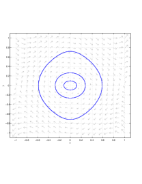
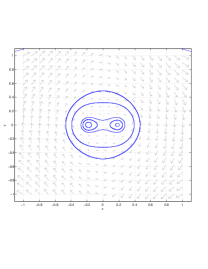
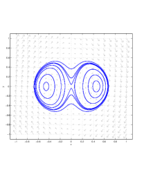
Figure 1. Symmetric state for $N-N_{cr}^{FD}<0$ corresponds to an equilibrium elliptic point $(\alpha,\beta)=(0,0)$ and asymmetric states for $N-N_{cr}^{FD}>0$ correlate to equilibrium points at $(\alpha,\beta)=(\pm\alpha_{cr},0)$. Plotted phase portrait corresponds to parameter values $\omega_{0}-\omega_{1}=.1$ and $N=.1,.2,.5$ respectively.

Appendix B Numerical Verification of Hypotheses

For a potential well

$$V(x)=\phi_{\sigma}(x-L)+\phi_{\sigma}(x+L)$$

with

$$\phi_{\sigma}(x)=\frac{e^{-\frac{x^{2}}{2*\sigma^{2}}}}{\sqrt{2\pi\sigma^{2}}},$$

where $\sigma=.001$, $L=7.5$. We discretize using a finite element method as in [MW] on a finer and finer set of grids that are concentrated near the peaks of the delta functions, we compute using the standard eigenvalue and eigenfunction solvers from Matlab the values from (1.2), (1.3) from hypothesis $(H4)$ are computed as

$$5\langle\psi_{0}^{4},\psi_{1}^{2}\rangle-\langle\psi_{0}^{6},1\rangle\approx.3305$$

and

$$20\frac{5\langle\psi_{0}^{4},\psi_{1}^{2}\rangle^{2}-\langle\psi_{0}^{6},1\rangle\langle\psi_{0}^{2},\psi_{1}^{4}\rangle}{5\langle\psi_{0}^{4},\psi_{1}^{2}\rangle-\langle\psi_{0}^{6},1\rangle}\!\!\!\!\! + \!\!\!\!\!160\frac{\langle\psi_{0}^{4},\psi_{1}^{2}\rangle^{2}}{\langle\psi_{0}^{6},1\rangle}-60\langle\psi_{0}^{2},\psi_{1}^{4}\rangle$$

$$\approx 9.9143$$

respectively, showing that computationally at least our hypotheses are valid for a particularly interesting symmetric potential.

References

• [BP1] V.Buslaev, G.Perelman, Scattering for the nonlinear Schrödinger equation: states close to a soliton, St. Petersburg Math.J., 4 (1993), pp. 1111–1142.
• [BP2] V.Buslaev, G.Perelman, On the stability of solitary waves for nonlinear Schrödinger equations, Nonlinear evolution equations, editor N.N. Uraltseva, Transl. Ser. 2, 164, Amer. Math. Soc., pp. 75–98, Amer. Math. Soc., Providence (1995).
• [CK] M.Christ, A.Kieslev, Maximal functions associated with filtrations, J. Funct. Anal. 179 (200). pp.s 409–425.
• [Cu1] S.Cuccagna, The Hamiltonian structure of the nonlinear Schrödinger equation and the asymptotic stability of its ground states, arXiv:0910.3797.
• [Cu2] S.Cuccagna, On asymptotic stability in energy space of ground states of NLS in 1D, J. Differential Equations, 245 (2008), pp. 653-691
• [Cu3] S.Cuccagna, A revision of ”On asymptotic stability in energy space of ground states of NLS in 1D”, arXiv:0711.4192 .
• [Cu4] S.Cuccagna, Stability of standing waves for NLS with perturbed Lamé potential, J. Differential Equations, 223 (2006), pp. 112-160
• [CM] S.Cuccagna, T.Mizumachi, On asymptotic stability in energy space of ground states for Nonlinear Schrödinger equations, Comm. Math. Phys., 284 (2008), pp. 51–87.
• [CPV] S.Cuccagna, D.Pelinovsky, V.Vougalter, Spectra of positive and negative energies in the linearization of the NLS problem, Comm. Pure Appl. Math. 58 (2005), pp. 1–29.
• [CT] S.Cuccagna, M.Tarulli, On asymptotic stability of standing waves of discrete Schrödinger equation in $Z$ , SIAM J. Math. Anal. 41, (2009), pp. 861-885
• [DMW] V.Duchêne, J.L.Marzuola and M.I.Weinstein, Wave operator bounds for $1$-dimensional Schrödinger operators with singular potentials and applications, to appear in J. Math. Phys. (2011).
• [GS] Zhou Gang, I.M.Sigal, Relaxation of Solitons in Nonlinear Schrödinger Equations with Potential , Advances in Math., 216 (2007), pp. 443-490.
• [GSc] M.Goldberg, W.Schlag, Dispersive estimates for Schrödinger operators in dimensions one and three, Comm. Math. Phys., 251 (2004), pp. 157–178.
• [H] E.M. Harrell. Double Wells, Comm. Math. Phys., 75 (1980), 239-261.
• [K] T.Kato, Wave operators and similarity for some non-selfadjoint operators , Math. Annalen, 162 (1966), pp. 258–269.
• [KPS] P.G. Kevrekidis, D.E. Pelinovsky, A. Stefanov Asymptotic stability of small solitons in the discrete nonlinear Schrödinger equation in one dimension SIAM J. Math. Anal. 41 (2009),pp. 2010–2030.
• [KKSW] E.Kirr, P.G.Kevrekidis, E.Shlizerman, M.I.Weinstein. Symmetry breaking bifurcation in Nonlinear Schrödinger/Gross-Pitaevskii Equations SIAM J. Math. Anal. 40 (2008), no. 2, 566–604.
• [KKP] E.Kirr, P.G.Kevrekidis, D.E. Pelinovsky. Symmetry breaking bifurcation in Nonlinear Schrödinger equation with symmetric potentials, preprint ArXiv:1012.3921 (2010).
• [KS] J.Krieger, W.Schlag, Stable manifolds for all monic supercritical focusing nonlinear Schrödinger equations in one dimension, J. Amer. Math. Soc., 19 (2006), pp. 815–920.
• [MW] J.Marzuola, M.I.Weinstein , Long time dynamics near the symmetry breaking bifurcation for nonlinear Schrödinger / Gross-Pitaevskii equations , Discrete and Continuous Dynamical Systems- A, 28 (2010), pp. 1505–1554.
• [M] T.Mizumachi, Asymptotic stability of small solitons to 1D NLS with potential , Jour. of Math. Kyoto University, 48 (2008), pp. 471-497.
• [NVT] K.Nakanishi, T. Van Phan, T.P. Tsai, Small solutions of nonlinear Schrödinger equations near first excited states, arXiv:1008.3581 .
• [PS] D. Pelinovsky, A. Stefanov, Asymptotic stability of small gap solitons in the nonlinear Dirac equations, arXiv:1008.4514.
• [SW1] A.Soffer, M.I.Weinstein, Multichannel nonlinear scattering for nonintegrable equations , Comm. Math. Phys., 133 (1990), pp. 116–146
• [SW2] A.Soffer, M.I.Weinstein, Multichannel nonlinear scattering II. The case of anisotropic potentials and data , J. Diff. Eq., 98 (1992), pp. 376–390.
• [SW3] A.Soffer, M.I.Weinstein, Selection of the ground state for nonlinear Schrödinger equations , Rev. Math. Phys. 16 (2004), pp. 977–1071.
• [TY] T.P.Tsai, H.T.Yau, Classification of asymptotic profiles for nonlinear Schrödinger equations with small initial data, Adv. Theor. Math. Phys. 6 (2002), pp. 107–139.
• [W] M.I.Weinstein, Lyapunov stability of ground states of nonlinear dispersive equations, Comm. Pure Appl. Math. 39 (1986), pp. 51–68.