Hole Dispersions for Antiferromagnetic Spin-$\frac{1}{2}$ Two-Leg Ladders by Self-Similar Continuous Unitary Transformations

Abstract

The hole-doped antiferromagnetic spin-$\frac{1}{2}$ two-leg ladder is an important model system for the high-$T_{c}$ superconductors based on cuprates. Using the technique of self-similar continuous unitary transformations we derive effective Hamiltonians for the charge motion in these ladders. The key advantage of this technique is that it provides effective models explicitly in the thermodynamic limit. A real space restriction of the generator of the transformation allows us to explore the experimentally relevant parameter space. From the effective Hamiltonians we calculate the dispersions for single holes. Further calculations will enable the calculation of the interaction of two holes so that a handle of Cooper pair formation is within reach.

I Introduction

The hole-doped antiferromagnetic spin-$\frac{1}{2}$ two-leg ladder is used as a model system, theoretically as well as experimentally, for the two-dimensional cuprate superconductors. Because the spin ladder is quasi one-dimensional it can more easily be treated by numerical and analytical approaches than the full two-dimensional model. For this reason the spin ladder was subject to many theoretical investigations in recent years Dagotto and Moreo (1988); Dagotto et al. (1992); Barnes et al. (1993); Dagotto and Rice (1996); Troyer et al. (1996); White and Scalapino (1997); Jeckelmann et al. (1998); Oitmaa et al. (1999); Sushkov (1999); Johnston et al. (2000); Brunner et al. (2001); Jurecka and Brenig (2001, 2002); Schmidt and Uhrig (2005); Roux et al. (2005); Bouillot et al. (2011). From a strong coupling perspective it is reasonable to describe the doped spin ladder by a $t$-$J$-model Harris and Lange (1967); Zhang and Rice (1988).

In this paper, our aim is to derive an effective Hamiltonian which describes not only the motion of the magnetic degrees of freedom, i.e., the triplons Schmidt and Uhrig (2003), but also of the charges, i.e., of the doped holes. This task is more challenging than the description of the triplons alone because the two kinds of excitations interact strongly and their energy ranges are not separated but they strongly overlap. Hence the excitations are not infinitely long-lived but they decay, at least in certain regions of the Brillouin zone.

The technique employed here is the approach of self-similar continuous unitary transformations (SCUT). In this approach the mapping of the true ground state to a vacuum of elementary excitations is constructed systematically, details will be explained in Sect. III. The basic idea is to implement a transformation that adjusts itself during the procedure of the diagonalisation depending on the current form of the Hamiltonian at this instant of the continuous transformation. The change of the Hamiltonian induced by the transformation is determined by the current magnitude of the non-diagonal elements. The flowing Hamiltonian is given in second quantization, i.e., it has a certain structure in terms of elementary creation and annihilation operators Knetter et al. (2003). This formulation incorporates the linked cluster property J. Oitmaa and Zheng (2006) automatically. The SCUT systematically defines a set of differential equations for the prefactors of the monomials of the creation and annihilation operators.

The key issue is to construct the flow to the effective Hamiltonian in a robust way. Due to the energetically overlapping states this goal required modifications Fischer et al. (2010) with respect to the previously performed unitary transformations. Thereby we achieved the successful calculation of the dispersion of a single hole.

In Sects. IV and V we investigate the dispersions of single hole excitations obtained from the effective Hamiltonians, which are results of the SCUT. We also compare our results to the results of other methods.

Sects. VI and VII conclude this article with a summary and perspectives for future work.

II Spin-$\frac{1}{2}$ Ladders

\psfrag{u}{u}\psfrag{l}{l}\psfrag{ri}{$n$}\psfrag{ri1}{$n+1$}\psfrag{Js}{$J_{\perp},t_{\perp}$}\psfrag{Jp}{$J_{\parallel},t_{\parallel}$}\psfrag{Jc}{$J_{\square}$}\includegraphics[scale={0.6}]{fig1.eps}

Figure 1: Spin-$\frac{1}{2}$ ladder consisting of the upper leg u, the lower leg l and the rungs $n$. The magnetic couplings are the nearest neighbor coupling on the rungs $J_{\perp}$, the nearest neighbor coupling along the legs $J_{\parallel}$ and the four spin coupling $J_{\square}$ for the ring exchange. The nearest neighbor hopping is described by the constants $t_{\perp}$ (on the rungs) and $t_{\parallel}$ (along the legs). The symmetry axis of the ladder is depicted by the dashed line.

The spin-$\frac{1}{2}$ ladder is realised in the so called telephone number compounds $\mathrm{(Sr,La,Ca,Y)}_{14}\mathrm{Cu}_{24}\mathrm{O}_{41}$ Vuletić et al. (2006). For these systems superconductivity can be detected under high pressure Uehara et al. (1996). Interactions between the ladders are weak because they result from $90^{\circ}$ exchange Gopalan et al. (1994); Matsuda et al. (2000). Thus the ladders can be considered to be isolated from one other. Even if the interladder coupling is taken into account, the strong frustration of the lattice causes the system to be effectively one-dimensional Schmidt and Uhrig (2007). The dispersions of the magnetic excitations of the complete layer with interladder coupling are similar to those of a single spin ladder. Important magnetic properties of the ladders are investigated in Refs. Dagotto and Moreo, 1988; Dagotto et al., 1992; Barnes et al., 1993; Dagotto and Rice, 1996; Johnston et al., 2000; Schmidt and Uhrig, 2005.

The focus of the present article is the lightly doped spin ladder because this will allow us to address the dynamics of charges. Of course, this system has been investigated previously by many techniques, for instance exact diagonalization Troyer et al. (1996); Roux et al. (2005), density-matrix renormalization White and Scalapino (1997); Jeckelmann et al. (1998); Roux et al. (2005), high-order series expansion Oitmaa et al. (1999), diagrammatic approaches Sushkov (1999); Jurecka and Brenig (2001, 2002), and quantum Monte Carlo Brunner et al. (2001). Hence much is known about the dynamics of a single hole, i.e., its dispersion, its spectral density and to some extent also about the bound states of two holes. The aim of the present paper is to establish an approach which generates an effective model for the motion of holes and their interaction with magnetic excitations and other holes. Such a model can be expressed in terms of creation and annihilation operators which create and annihilate holes, i.e., charge excitations, and triplons, i.e., magnetic excitations. The techniques used so far do not yield such an effective model but numerical data for eigen energies and spectral weights. For this reason we here use the complementary approach of self-similar continuous unitary transformations.

The spin sites in our model (see Fig. 1) are the $3d_{x^{2}-y^{2}}$ orbitals of the copper atoms coupled via the $2p_{x}$ or $2p_{y}$ orbitals of the oxygen atoms, which hybridise with the copper $3d_{x^{2}-y^{2}}$ orbitals so that an antiferromagnetic superexchange Anderson (1950) is possible. The Hamiltonian in the usual form of a $t$-$J$-model, for derivations see Ref. Hamerla et al., 2010 and references therein, reads

$$H = J_{\perp}\sum_{n}\vec{S}_{n,\mathrm{u}}\cdot\vec{S}_{n,\mathrm{l}}+J_{\parallel}\sum_{n,\alpha=\mathrm{u,l}}\vec{S}_{n,\alpha}\cdot\vec{S}_{n+1,\alpha}$$

$$+J_{\square}\sum_{n}\left[\left(\vec{S}_{n,\mathrm{u}}\cdot\vec{S}_{n+1,\mathrm{u}}\right)\left(\vec{S}_{n,\mathrm{l}}\cdot\vec{S}_{n+1,\mathrm{l}}\right)\right.$$

$$+\left(\vec{S}_{n,\mathrm{u}}\cdot\vec{S}_{n,\mathrm{l}}\right)\left(\vec{S}_{n+1,\mathrm{u}}\cdot\vec{S}_{n+1,\mathrm{l}}\right)$$

$$\left.-\left(\vec{S}_{n,\mathrm{u}}\cdot\vec{S}_{n+1,\mathrm{l}}\right)\left(\vec{S}_{n,\mathrm{l}}\cdot\vec{S}_{n+1,\mathrm{u}}\right)\right]$$

$$-t_{\perp}\sum_{n,\alpha=\mathrm{u,l}}c^{\dagger}_{\sigma,\alpha,n}c^{\phantom{\dagger}}_{\sigma,\overline{\alpha},n}-t_{\parallel}\sum_{n,\alpha=\mathrm{u,l}}c^{\dagger}_{\sigma,\alpha,n}c^{\phantom{\dagger}}_{\sigma,\alpha,n\pm 1}.$$

The nearest neighbor terms with the couplings $J_{\perp}$ and $J_{\parallel}$ (see Fig. 1) are not sufficient to describe the magnetic interactions in the system. Because the hybridization path around the $\mathrm{Cu}_{4}\mathrm{O}_{4}$ square plaquettes is strong, the influence of the four-spin interactions belonging to these plaquettes (i.e. two neighboring rungs) is not negligible Coldea et al. (2001). These interactions are referred to as ring exchange (also cyclic exchange) with the coupling $J_{\square}$ (see Fig. 1). Actually the complete ring exchange also includes two-spin terms for all two-spin combinations of the four spins on two neighboring rungs. Yet the contributions from the terms coupling the spins along the rungs and parallel to the legs are merged with the nearest neighbor terms so that the coupling constants $J_{\perp}$ and $J_{\parallel}$ include these contributions, whereas the terms coupling the spins diagonally can be neglected because their prefactor is only of the order of $3\%$ of $J_{\perp}$ Mizuno et al. (1999). The complete representation of the ring exchange using spin operators can be found in Ref. Brehmer et al., 1999.

The hopping of the spins is described by the constants $t_{\perp}$ and $t_{\parallel}$ (see Fig. 1). The creation and annihilation operators $c^{\dagger}$ and $c^{\phantom{\dagger}}$ already incorporate hardcore properties so that double occupancy is forbidden.

We define the dimensionless quantities

$$x=\frac{J_{\parallel}}{J_{\perp}},\,x_{\square}=\frac{J_{\square}}{J_{\perp}},\,\lambda_{\perp}=\frac{t_{\perp}}{J_{\perp}},\,\lambda_{\parallel}=\frac{t_{\parallel}}{J_{\perp}},$$ (2)

which are normalized to $J_{\perp}$.

It is convenient to treat the ladder as a one-dimensional chain of rungs. There are nine possible local states on a rung $n$ of the ladder.

$$\left|s\right\rangle_{n}=\frac{1}{\sqrt{2}}\left(\left|\uparrow\downarrow\right\rangle-\left|\downarrow\uparrow\right\rangle\right)_{n}$$ (3a)

$$\left|t_{x}\right\rangle_{n}=\frac{-1}{\sqrt{2}}\left(\left|\uparrow\uparrow\right\rangle-\left|\downarrow\downarrow\right\rangle\right)_{n}$$ (3b)

$$\left|t_{y}\right\rangle_{n}=\frac{\mathrm{i}}{\sqrt{2}}\left(\left|\uparrow\uparrow\right\rangle+\left|\downarrow\downarrow\right\rangle\right)_{n}$$ (3c)

$$\left|t_{z}\right\rangle_{n}=\frac{1}{\sqrt{2}}\left(\left|\uparrow\downarrow\right\rangle+\left|\downarrow\uparrow\right\rangle\right)_{n}$$ (3d)

$$\left|a_{\tau=1,\sigma=1}\right\rangle_{n}=\frac{1}{\sqrt{2}}\left(\left|\uparrow 0\right\rangle+\left|0\uparrow\right\rangle\right)_{n}$$ (3e)

$$\left|a_{\tau=-1,\sigma=1}\right\rangle_{n}=\frac{1}{\sqrt{2}}\left(\left|\uparrow 0\right\rangle-\left|0\uparrow\right\rangle\right)_{n}$$ (3f)

$$\left|a_{\tau=1,\sigma=-1}\right\rangle_{n}=\frac{1}{\sqrt{2}}\left(\left|\downarrow 0\right\rangle+\left|0\downarrow\right\rangle\right)_{n}$$ (3g)

$$\left|a_{\tau=-1,\sigma=-1}\right\rangle_{n}=\frac{1}{\sqrt{2}}\left(\left|\downarrow 0\right\rangle-\left|0\downarrow\right\rangle\right)_{n}$$ (3h)

$$\left|2h\right\rangle_{n}=\left|00\right\rangle_{n}$$ (3i)

The states without holes are the singlet (3a) and the triplet states (3b-3d), for which we use the representation from Ref. Sachdev and Bhatt, 1990 because the symmetry in spin space is manifest in this representation. The states consisting of one hole and one spin $\frac{1}{2}$ (3e-3h) have the quantum numbers $\tau$, which is the parity of the state with respect to the symmetry axis of the ladder (see dashed line in Fig. 1), and $\sigma$, which indicates whether the $S_{z}$ component of the spin is up or down. The double hole state (3i) is neglected here because only one-hole states will be considered. The local energy of $\left|2h\right\rangle$ is also larger than the energy of the other states. Therefore $\left|2h\right\rangle$ is expected to be also less important for ladders with low, but macroscopic doping, though it will influence the quantitative results for hole-hole scattering and hole-hole binding.

For the application of the continuous unitary transformation a representation using the creation and annihilation operators for the local states (3a-3h) is indicated. The complete Hamiltonian (II) in the respresentation using these operators can be found in Ref. Duffe, 2010. Note that the local rung states incorporate hardcore properties. Also the fermionic states exhibit additional hardcore properties which simply result from the fact that each rung can only be in one particular state.

The excitations are actually dominated by the local states as long as the couplings between the rungs are small. The magnetic excitations are triplons, i.e., triplet states dressed with the magnetic interactions with their environment Schmidt and Uhrig (2003). We do not want to use the term “magnon” for these magnetic excitations because this term is usually associated with quasiparticles in systems that exhibit long-range magnetic order (which is not the case for the spin ladder). Moreover triplons feature the appropriate threefold degeneracy based on their $S=1$ character Schmidt and Uhrig (2003).

III SCUT

We use the method of continuous unitary transformations (CUT) to obtain an effective Hamiltonian Głazek and Wilson (1993); Wegner (1994); Kehrein (2006). Instead of applying only a single constant unitary transformation that diagonalises the Hamiltonian at once or several constant unitary transformations successively, a unitary transformation depending on a continuous parameter is applied to the Hamiltonian. This transformation adjusts itself permanently during its application. Discrete transformations must be known explicitly before we can apply them, whereas for the continuous transformation it is sufficient to set up the infinitesimal generator of the transformation. The unitary operator $U$ depending on the continuous parameter $l$ transforms the Hamiltonian by

$$H(l)=U(l)HU^{\dagger}(l).$$ (4)

The generator of the transformation is defined by

$$\eta(l)=\frac{\partial U(l)}{\partial l}U^{\dagger}(l).$$ (5)

The generator defines the properties of the transformation. The derivative of $H$ with respect to $l$ is given by the so-called flow equation

$$\frac{\partial H(l)}{\partial l}=\left[\eta(l),H(l)\right]\,\mathrm{.}$$ (6)

This is actually a system of differential equations (generically highly coupled) for the coefficients of the operators appearing in $H(l)$. To achieve the effective Hamiltonian the flow equation has to be solved. For a self-similar application of the CUT Mielke (1997); Reischl et al. (2004); Fischer et al. (2010) the Hamiltonian is represented by a sum of different operators $\hat{o}_{i}$, which are products of local operators in second quantization, multiplied by prefactors $g_{i}$.

$$H(l)=\sum_{i}g_{i}(l)\hat{o}_{i}$$ (7)

The operators $\hat{o}_{i}$ determine the structure of $H(l)$. This is the reason why this formulation of the CUTs is called self-similar. In particular, we express the operators $\hat{o}_{i}$ in terms of creation and annihilation operators of charge excitations (holes) and spin excitations (triplons) in the manner introduced previously Knetter et al. (2003). A reference state, the vacuum, has to be chosen with respect to which these creation and annihilation processes are defined. In our case, this state is the product of local singlets on the rungs of the ladder. For the undoped ladder this state is a convenient starting point as seen in many high-order perturbative Uhrig and Schulz (1996); Trebst et al. (2000); Knetter et al. (2001) and diagrammatic approaches Jurecka and Brenig (2001, 2002). Since we focus in this work on single hole dynamics the use of the product of local singlets on the rungs as reference vacuum is well justified.

The differential equations for the $g_{i}(l)$ are given by the flow equation in the form

$$\frac{\partial g_{i}(l)}{\partial l}=\sum_{j,k}a_{i,j,k}g_{j}(l)g_{k}(l).$$ (8)

Because an infinite system yields an infinite number of differential equations which cannot be solved numerically, we have to apply a truncation to $H(l)$ so that a closed system of differential equations is obtained. We choose a real space truncation because the correlation length is finite for the spin ladder due to the energy gap Dagotto and Moreo (1988); Dagotto et al. (1992). The concrete truncation scheme is explained in Sect. III.3.

It should also be noted that the truncation is only restricted to operators. There is no truncation of the Hilbert space of the states. Thus although operators affecting higher numbers of particles are omitted, the number of particles that can be treated is arbitrarily large. To illustrate this we consider the action of a term in second quantisation, e.g., $a^{\dagger}_{i}a^{\dagger}_{j}a^{\phantom{\dagger}}_{k}$, which annihilates one particle and creates two. This term acts not only on the one-particle subspace, but also on the subspaces with more than one particle, e.g. it changes a four-particle into a five-particle state.

The solution of the flow equation is a rather straightforward numerical integration. The convergence is monitored during the integration. Since all contributions to the generator decrease in case of convergence, the absolute values of the concerning coefficients are squared and summed. The square root of this sum is defined as residual off-diagonality (ROD). It is the norm of the generator and also a measure for the convergence. The ROD is expected to tend to zero for $l\rightarrow\infty$. Note that the term “off-diagonality” is meant in a broader sense, i.e. the definition of the generator determines which elements shall be kept for $l\rightarrow\infty$ and these elements are defined as “diagonal” parts of the Hamiltonian. The RODs depicted in the following are always normalized to the initial ROD at $l=0$.

With the decrease of the ROD the wanted effective Hamiltonian is approached. If the relative ROD falls below a certain threshold specifying the precision of the result (usually $\approx 10^{-8}$), the integration can be considered to be completed. The number of coefficients treated in our actual calculations is of the order up to $10^{5}$ for the doped spin ladder.

III.1 Generator

\psfrag{l=0}{$l=0$}\psfrag{finite l}{finite $l$}\psfrag{l=inf}{$l=\infty$}\includegraphics[scale={0.4}]{fig2.eps}

Figure 2: (Color online) Schematic example for a transformation of $H(l)$ induced by the pc generator: Each coloured ($n_{c}$, $n_{a}$)-block represents contributions to $H$ creating $n_{c}$ particles after annihilating $n_{a}$ particles.

The particle conserving or pc generator

$$\eta_{\mathrm{pc},i,j}(l)=\mathrm{sign}(q_{i}-q_{j})H_{i,j}(l)$$ (9)

was introduced by Mielke for band matrices Mielke (1998) for $q_{i}=i$ and simultaneously by Knetter and Uhrig for many-body Hamiltonians where $q_{i}$ counts the number of elementary excitations Uhrig and Normand (1998); Knetter and Uhrig (2000). The indices $i$ and $j$ label the transition from state $j$ to state $i$. These states are eigenstates of an operator $Q$, which counts the number of elementary excitations, i.e., quasi-particles. The eigen value of $Q$ for the state $i$ is $q_{i}$.

The differences between the pc and the Wegner generator are discussed by means of simple Hamiltonians in Ref. Dusuel and Uhrig, 2004. In particular the convergence behavior is examined. The Wegner generator $\eta_{\text{Wegner}}=[H_{0},H]$ Wegner (1994) always leads to a fixed point, but it does not necessarily aim at a quasi-particle picture because degeneracies may hinder the diagonalisation. The pc generator is not sensitive to degeneracies, but the induced transformation does not always converge for infinite systems.

Due to the sign function the generator (9) contains only terms of the Hamiltonian that change the particle number. Terms which decrease the particle number acquire an additional minus sign. The resulting transformation yields an effective Hamiltonian for $l\rightarrow\infty$ which conserves the particle number (see Fig. 2). The asymptotic behavior Mielke (1998); Fischer et al. (2010) of the non-particle-conserving terms, i.e., $q_{i}\neq q_{j}$, is dominated by

$$\frac{\partial H_{i,j}(l)}{\partial l}\approx-\mathrm{sign}(q_{i}-q_{j})(H_{i,i}(l)-H_{j,j}(l))H_{i,j}(l)\,.$$ (10)

Because $H_{i,j}(l)$ tends to zero for $l\rightarrow\infty$ if $q_{i}\neq q_{j}$, the transformation tries to sort the eigenenergies $H_{i,i}$ according to the particle number $q_{i}$, i.e.,

$$\mathrm{sign}(q_{i}-q_{j})(H_{i,i}(l)-H_{j,j}(l))>0$$ (11)

holds true for large $l$.

Overlapping energies of states with different quasiparticles can hinder the convergence of the flow. This problem can be solved by excluding terms from the generator Fischer et al. (2010). The ground state or gs generator

$$\eta_{\mathrm{gs},i,j}(l)=(\delta_{j,0}-\delta_{i,0})H_{i,j}(l)$$ (12)

introduced in Ref. Fischer et al., 2010 includes only terms that couple to the vacuum $|i=0\rangle$ of excitations so that in the effective Hamiltonian only this vacuum is decoupled from the remaining Hilbert space. Then it has become the ground state. This is sufficient for the calculation of the hole dispersion for the spin ladder if the ground state can be continuously linked to the state without magnetic excitations for a given hole configuration. This is the case for a single hole at a given momentum close to the minimum of its band.

III.2 Real Space Restriction of the Generator

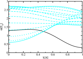
Figure 3: (Color online) Schematic example for an overlap between one- and two-particle energies. The black line is the one-particle dispersion, the solid cyan (gray) lines are the boundaries of the two-particle continuum and the dashed lines are the energies of the two-particle states which are actually affected by the terms $a^{\dagger}_{n}a^{\dagger}_{n+\Delta n}a_{m}$ and $a^{\dagger}_{m}a_{n+\Delta n}a_{n}$. The cyan (gray) dashed lines do not pose a problem because they do not cross the one-particle dispersion. Convergence problems can only be induced by the terms that act on the states with the cyan (gray) dotted dispersions, which cross the one-particle dispersion.

But even the gs generator encounters convergence problems if the interaction between the rungs becomes too strong, i.e., $x=1$, $\lambda_{\perp}=\lambda_{\parallel}>2$. Hence we have developed a generator adaption with a real space restriction of the generator terms.

Many terms that remain after the real space truncation of the Hamiltonian act on states with discrete energies within the continua (see Fig. 3). The divergence of the SCUT in case of an overlap is not induced by all terms that mediate between overlapping continua, but only by a part of these terms. Thus a stricter real space truncation of the Hamiltonian can induce convergence. However, a stricter truncation causes a larger error for the results of the SCUT.

Therefore we do not apply a stricter truncation to the Hamiltonian but we choose a stricter generator. We emphasize that a restriction of the generator does not imply an approximation. It only changes the direction of the unitary rotation. This restriction of the generator is not based on the total extension of the terms, but on the extension of the creation operators and on the extension of the annihilation operators separately.

Let us consider the example of an overlap between one- and two-particle energies shown in Fig. 3. The terms $a^{\dagger}_{n}a^{\dagger}_{n+\Delta n}a^{\phantom{\dagger}}_{m}$ and $a^{\dagger}_{m}a^{\phantom{\dagger}}_{n+\Delta n}a^{\phantom{\dagger}}_{n}$ are responsible for transitions between the one- and the two-particle subspace. We choose to restrict the generator based on $|\Delta n|$, which is the distance between the two particles which are created or annihilated. Because the one-particle state does not have an extension, it is not relevant for the restriction of the generator. All terms that have a larger $|\Delta n|$ than a certain $\Delta n_{\mathrm{max}}$ are excluded from the generator. Note that they are still part of the Hamiltonian as long as they meet the truncation criteria for the Hamiltonian.

The transformation induced by this restricted generator does not try to sort all eigenenergies (cf. Eq. 11), but only those which are captured by the terms in the generator. Therefore the flow may also converge in case of overlapping energies. The price to be paid is that the subspaces affected by the omitted terms are not completely decoupled from the remaining Hilbert space. Thus either an additional diagonalization or a diagrammatic analysis has to be applied to the effective Hamiltonian from this SCUT or the results have to be considered as upper limit for the actual results. The restriction of the generator can be applied to the pc generator or to any of its adaptions, e.g., to the gs generator.

III.3 Truncation Scheme

The finite energy gap $\Delta$ of the triplons Dagotto and Moreo (1988); Dagotto et al. (1992) is equivalent to a correlation function which is exponentially decreasing with respect to the distance. Hence a truncation in real space is appropriate. The extension in real space shall be used as a measure for the physical importance of a term of the Hamiltonian. In our quasi one-dimensional spin ladder the extension of a term is defined as the difference between the smallest and the largest rung index of the local operators within the term.

The simplest way of truncating would be one maximal extension in real space for all terms. Terms exceeding this limit would be omitted. But this approach is not reasonable in our case. The number of possible terms increases much more strongly with the maximal extension for terms consisting of more local operators. However, terms consisting of less operators are usually more important. Hence higher extensions should be taken into account for terms with less operators. For instance, the coefficient of a one-particle hopping term consisting of two local operators is usually larger than the coefficient of a two-particle interaction term consisting of four local operators if they both have the same extension. Therefore, for the pure triplon terms different maximal extensions $d_{n}$ are defined in units of the rung distance where $n$ is the total number of local operators of the term under study. Because only terms changing the particle number by two or conserving the particle number occur in the initial magnetic Hamiltonian, only the $d_{n}$ with even $n$ are meaningful .

By $h_{n^{\prime}}$ we denote the maximal extension for $n^{\prime}$ hole state operators. It does not matter if the term concerned contains additional triplon operators. For terms with triplon and hole state operators, $h_{n^{\prime}}$ affects only the hole state operators. The total maximal extension $t_{n^{\prime\prime}}$ for these mixed terms depends on the number of triplon operators $n^{\prime\prime}$. The parameter $N_{t}$ denotes the maximal number of triplons interacting with holes. Note that $t_{n^{\prime\prime}}$ with odd $n^{\prime\prime}$ have to be taken into account because the triplon number is changed by an odd number if the hole state parity is altered.

Additionally a maximal triplon number $N$ and a maximal hole number $N_{h}$ are defined for the operators, i.e., terms affecting higher triplon numbers than $N$ or higher hole numbers than $N_{h}$ are completely omitted. This truncation scheme is not compulsory. Other schemes could be implemented which use different classifications for the groups of terms sharing the same maximal extension.

Since the size of the system of differential equations for the doped ladder grows exponentially with increasing extensions, the truncation for our calculations is fairly strict. The parameters $N=4$, $d_{2}=10$, $d_{4}=6$, $d_{6}=4$ and $d_{8}=3$ were used for the pure triplon terms because these maximal extensions are sufficient for the undoped case up to $x=1$.

For the terms including hole operators the truncation used for the SCUT is given by $N_{h}=1$, $N_{t}=2$, $h_{2}=3$, $t_{1}=6$, $t_{2}=6$, $t_{3}=5$, $t_{4}=5$, $t_{5}=4$ and $t_{6}=4$. All results shown in the sequel are obtained with these parameters unless stated otherwise.

IV Hole Dispersions without Ring Exchange

IV.1 Calculations with Unrestricted Generators

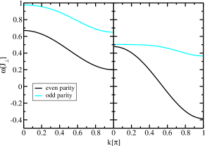
Figure 4: (Color online) One-hole dispersion for $x=x_{\square}=0$ calculated with the pc generator; left: $\lambda=0.25$, right: $\lambda=0.5$. The curves coincide well with the series expansion results from Oitmaa et al., 1999.

The dispersion of a single hole in the absence of triplons can be easily derived from the effective Hamiltonian by means of Fourier transformation. The part of the Hamiltonian to be diagonalised

$$H_{\mathrm{1h}}=\sum_{d=-h_{2}}^{h_{2}}\sum_{\tau,\sigma,n}b_{d}\,a^{\dagger}_{\tau,\sigma,n+d}a^{\phantom{\dagger}}_{\tau,\sigma,n}$$ (13)

contains the one-hole terms restricted by $h_{2}$ and characterised by the coefficients $b_{d}$. The one-hole dispersion

$$\omega_{\mathrm{1h},\tau}(k)=b_{0}+\sum_{d=1}^{h_{2}}2b_{d}\cos(dk)$$ (14)

only depends on the parity $\tau$ and it is degenerate concerning the spin $\sigma$.

If $\lambda_{\parallel}$ and $\lambda_{\perp}$ are small while $x=x_{\square}=0$, the dispersion reads

$$\frac{\omega_{\mathrm{1h},\pm 1}(k)}{J_{\perp}}=\frac{3}{4}\mp\lambda_{\perp}+\lambda_{\parallel}\cos(k)+\mathcal{O}(\lambda_{\perp}^{2},\lambda_{\parallel}^{2},\lambda_{\perp}\lambda_{\parallel}).$$ (15)

In the following we only consider the isotropic case $\lambda_{\perp}=\lambda_{\parallel}=\lambda$. For small values of the parameters $x$, $x_{\square}$ and $\lambda$ the deviations from Eq. (15) are actually small. In Fig. 4 two values of $\lambda$ are considered for $x=x_{\square}=0$. The result for $\lambda=0.25$ already exhibits deviations from the relation (15) for small hopping constants. Both bandwidths are smaller than $2\lambda=0.5$. The odd band is narrower than the even band. Moreover the odd band is shifted upwards by less than $\lambda$, while the even band is shifted downwards by slightly more than $\lambda$.

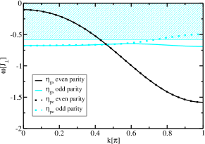
Figure 5: (Color online) One-hole dispersion for $x=x_{\square}=0$, $\lambda=1$ calculated with the gs generator and the pc generator. The results for the even bands coincide so that the curves cannot be distinguished. The cyan (gray) shaded area is the continuum formed by one triplon and one even hole state.

The increase of $\lambda$ to $0.5$ yields a result with obvious deviations relative to Eq. (15). The odd band becomes lower and narrower with growing $\lambda$ in this region. The cosine shape of both dispersions is – for $\lambda=0.25$ as well as for $\lambda=0.5$ – not deformed by higher harmonics. The results of the series expansion Oitmaa et al. (1999) exhibit the same behavior for these parameters in good agreement with the SCUT results. However, it has to be pointed out that the convergence of the SCUT is much worse for $\lambda=0.5$ than for $\lambda=0.25$. The residual off-diagonality (ROD) defined in Sect. III and used as a measure for the convergence is decreasing very slowly for $\lambda=0.5$. While the ROD is smaller than $10^{-6}$ at $lJ_{\perp}=200$ for $\lambda=0.25$, it is still larger than $10^{-3}$ at $lJ_{\perp}=200$ for $\lambda=0.5$. Both RODs are decreasing exponentially for large $l$. Theses RODs are not shown here.

For $x=x_{\square}=0$, $\lambda=1$ the pc generator yields results for the even band that still agree very well with the series expansion. For the odd band there are no series expansion results available. Fig. 5 shows the comparison of the results for the pc generator and for the gs generator. The even band results lie on top of each other, but the odd band exhibits deviations for $k\gtrsim 0.57\pi$. While the gs generator produces an almost featureless dispersion (compared to the even band), the pc generator causes a pronounced maximum at $k=\pi$. These differences are due to the position of the lower boundary of the continuum formed by one triplon and one even hole state (see also Fig. 5). This is the odd continuum due to the odd parity of the triplon. An overlap between the odd dispersion and this continuum is present for the pc result. The deviating odd band from the gs generator avoids this overlap. For both generators the even and the odd band cross at $k\approx 0.46\pi$. While the even band keeps its cosine shape, the second harmonic for the odd band is no longer negligible for both the pc and the gs generator.

Figure 6: ROD for the SCUT for $x=x_{\square}=0$, $\lambda=1$ induced by the pc generator (solid line) and by the gs generator (dashed line).

For $x=x_{\square}=0$, $\lambda=1$ the transformation does not converge for the pc generator, while the gs generator induces convergence (see Fig. 6). The overlap hinders the convergence for the pc generator. The kink at $lJ_{\perp}\approx 120$ in the gs ROD is probably due to numerical inaccuracies that are amplified via a feedback within the flow equation. Since the relative ROD is already $\approx 10^{-7}$ at the kink we can stop the transformation at this point and neglect the remaining off-diagonal terms, i.e., we consider the transformation to be converged. For the calculation of the hole dispersions the pc SCUT was stopped at $lJ_{\perp}\approx 50$ where the ROD is still $\approx 10^{-2}$ and thus not negligible. Therefore the result from the gs generator is more trustable than the result from the pc generator. The parameters $x=x_{\square}=0$, $\lambda=2$ lead to divergence for either generator.

IV.1.1 Finite Coupling Ratio $x=J_{\parallel}/J_{\perp}$

Here we want to consider $x>0$. For $\lambda=0$ the energy of the hole states, which is independent of momentum $k$ and parity $\tau$, decreases with increasing $x$. Already for small finite $\lambda$ the deviations from the simple cosine shape appear for the odd band. This can be seen in Fig. 7 where the one-hole dispersions for $x=0.5$ and $\lambda=0.25$ are depicted. The odd band agrees well with the series expansion; only slight deviations at $k=0$ occur. For the even band no series expansion data are available.

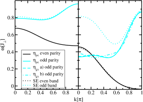
Figure 7: (Color online) Left panel: One-hole dispersion for $x=0.5$, $x_{\square}=0$, $\lambda=0.25$ calculated with the pc generator. The series expansion result for the odd band is also shown, while the result for the even band is not available. Right panel: One-hole dispersion for $x=0.5$, $x_{\square}=0$, $\lambda=0.5$ calculated with the pc generator and the gs generator. For case a) in the legend the usual truncation was used. For case b) in the legend $h_{2}$ was increased to $4$, $t_{1}$ and $t_{2}$ to $8$ as well as $t_{3}$ and $t_{4}$ to $6$. The dotted curves are extrapolations from the series expansion data.

For $x=0.5$ and $\lambda=0.5$ , see also Fig. 7, the result for the even band agrees again well with the series expansion result Oitmaa et al. (1999), but the odd band behaves differently. Only for large $k$ the behavior is similar although also in this region the SCUT result is slightly lower. The series expansion result exhibits a local maximum at $k=0$ and a global minimum at $k\approx 0.58\pi$, while the SCUT result hardly changes in the region $0<k<\frac{\pi}{2}$. The gs generator yields the same result as the pc generator apart from minimal deviations ($<2\%$) at $k=0$. However, the gs generator allows us to extend the truncation scheme: $h_{2}$ was increased to $4$, $t_{1}$ and $t_{2}$ to $8$ as well as $t_{3}$ and $t_{4}$ to $6$. In the result the shape of the odd band changes mainly for small $k$. Thus the odd dispersion still changes with increasing maximal extensions.

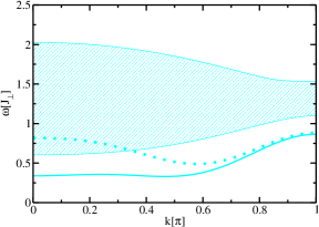
Figure 8: (Color online) Comparison of the odd hole dispersion and the continuum formed by one triplon and one even hole state for $x=0.5$, $x_{\square}=0$, $\lambda=0.5$. The odd hole dispersion was derived from SCUT using the pc generator (cyan/gray solid) and by series expansion (cyan/gray dotted). The cyan (gray) shaded area is the continuum (derived from the same SCUT calculation).

We can understand these differences between SCUT and series expansion by looking at the position of the continuum formed by one triplon and one even hole state (see Fig. 8). The series expansion result crosses the lower boundary of this continuum at $k\approx 0.34\pi$. Assuming that the series expansion yields a result close to the actual odd hole dispersion it is cogent that the SCUT based on the pc generator is not able to sort the eigen values properly for small $k$ because creating one triplon does not necessarily increase the energy.

Since the problematic overlap concerns the zero- and the one-triplon space, the use of the gs generator is no remedy here. This may come as a surprise at first since it was shown in Ref. Fischer et al., 2010 that the gs generator always implies a robust flow. This statement applies if the hole is put in its band minimum because this is by construction the lowest eigen state of the ladder doped with one hole. But for other energies of the hole dispersion this does not need to be the case so that the energy of one hole may lie higher than the energy of one hole and one triplon. Hence the gs generator yields mainly the same result and suffers from the same problems as the pc generator. A robust extrapolation of the series can still yield reasonable results because the series is not fully sensitive to the overlap of states at higher values of the expansion parameters.

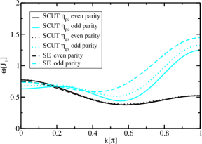
Figure 9: (Color online) One-hole dispersion for $x=1$, $x_{\square}=0$, $\lambda=0.5$ calculated with the pc generator and the gs generator. The dashed curves are extrapolations from the series expansion data.

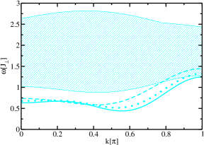
Figure 10: (Color online) Comparison of the odd hole dispersion and the continuum formed by one triplon and one even hole state for $x=1$, $x_{\square}=0$, $\lambda=0.5$. The odd hole dispersion was derived from SCUT using the pc generator (cyan/gray solid), using the gs generator (cyan/gray dotted) and by series expansion (cyan/gray dashed). The cyan (gray) shaded area is the continuum (derived from the same pc SCUT calculation).

For $x=1$ and $\lambda=0.5$ (see Fig. 9) the SCUT results for the odd band again show distinct deviations from the series expansion results. The even band exhibits a maximal deviation at $k=0$ of only $\approx 1\%$. The deviations of the energetically higher odd band are larger, but still well tolerable for the gs generator. All in all the deviations are not as pronounced as for $x=0.5$ and $\lambda=0.25$. A comparison with the continuum formed by one even hole and one triplon (see Fig. 10) shows that an overlap exists around $k=\pi$ for the series expansion result and for the gs result. This explains again the deviations in this region. As this overlap is not as strong as the overlap for $x=0.5$ and $\lambda=0.5$ the deviations are smaller. Even if there is no actual overlap, the continuum is at least very close. Hence it is to be expected that the actual odd hole dispersion is lowered for $k\approx\pi$ due to this reason.

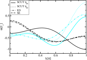
Figure 11: (Color online) One-hole dispersion for $x=1$, $x_{\square}=0$, $\lambda=1$ calculated with the pc generator and the gs generator. The dashed curve is the result from the series expansion, for which only the even band is available. The dashed-dotted curves are exact diagonalization results.

For $x=1$ and $\lambda=1$ (see Fig. 11) no one-hole dispersion with odd parity is available from series expansion. Thus we look at the even band including results from exact diagonalization. For the exact diagonalization a finite ladder with $14$ rungs was examined and the resulting eigenenergies were fitted by a sum of three cosine terms for both bands, see Eq. (14). The pc result for the even band differs completely from the gs result. For the odd band the pc result lies below the gs result and the deviations grow with increasing momentum. The comparison with the series expansion and with the exact diagonalization suggests that the gs result is more reliable because the deviations are smaller than $1\%$ for the even band. Also for the odd band the gs result is closer to the exact diagonalization result. The odd band is more difficult to assess due to the vicinity to the odd continuum.

It should be noted that the diagrammatic approach from Ref. Jurecka and Brenig, 2001 yields bands that show qualitative deviations from the SCUT and from the exact diagonalization concerning the shape for small $k$. The authors state that this regime actually exceeds the applicability of their approach. The quantum Monte Carlo result from Ref. Brunner et al., 2001 is in very good agreement with our result. For the even band the agreement is even excellent and comparable to the agreement between SCUT and exact diagonalization.

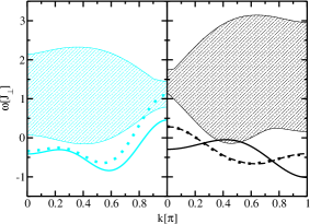
Figure 12: (Color online) Comparison of the hole dispersions and the continua formed by one triplon and one hole state for $x=1$, $x_{\square}=0$, $\lambda=1$. Left: The odd hole dispersion was derived from SCUT using the pc generator (cyan/gray solid) and using the gs generator (cyan/gray dotted). The cyan (gray) shaded area depicts the continuum with one even hole and one triplon derived from the same gs SCUT calculation. Right: The even hole dispersion was derived from SCUT using the pc generator (black solid), using the gs generator (black dotted) and by series expansion (black dashed). The black shaded area depicts the continuum with one odd hole and one triplon derived from the same gs SCUT calculation.

The odd band result from the gs SCUT enters the continuum formed by one triplon and one even hole state for $k\gtrsim 0.83\pi$ (see Fig. 12), while the pc result lies always below this continuum. This overlap is also present in the exact diagonalization result and in the quantum Monte Carlo result Brunner et al. (2001). A comparison of the even one-hole dispersion and the even continuum formed by one triplon and one odd hole state (see also Fig. 12) supports the assumption that the gs result is more reliable than the pc result. The dispersion induced by the gs SCUT exhibits a shape that appears as if it were formed by the lower boundary of the approaching continuum. This is plausible because the vicinity of the continuum lowers the dispersion. The pc result, however, stays away from the continuum at $k=0$ and at the boundary of the Brillouin zone. The overlap with the continuum around $k\approx 0.44\pi$ occurs in the pc calculation only due to truncation.

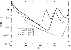
Figure 13: ROD for the SCUT calculated with the pc generator for various parameters.

At this point we compare the convergence behavior for $x=0.5$, $\lambda=0.5$; $x=1$, $\lambda=0.5$ and $x=1$, $\lambda=1$ for the pc generator. The corresponding RODs are depicted in Fig. 13. All three curves exhibit a kink with non-converging behavior afterwards. This is typical for cumulating rounding errors because of a symmetry breaking due to numerical inaccuracies. Such a symmetry breaking is not unlikely because the full spin symmetry could not be used explicitly.

It is surprising that the ROD for $x=1$, $\lambda=0.5$ reaches a lower minimum than the one for the lower parameter set $x=0.5$, $\lambda=0.5$. This seems to contradict the expectation that larger values of the interdimer processes imply a more difficult CUT. But inspecting the slope of the RODs in Fig. 13 before reaching their minima one sees that these slopes, i.e., the convergence velocities, are indeed largest for the smallest values for the interdimer processes.

IV.1.2 Strong Hopping $\lambda=t/J_{\perp}>1$

For $x=1$ and $\lambda>1$ the parameters are entering a region which is expected to reflect realistic relations of the constants in the telephone number compounds. The results for $x=1$ and $\lambda=2$ are shown in Fig. 14. Again we compare with results from series expansion and from exact diagonalization for $14$ rungs.

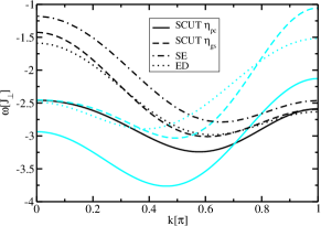
Figure 14: (Color online) One-hole dispersion for $x=1$, $x_{\square}=0$, $\lambda=2$ calculated with the pc generator and the gs generator. The graph also shows the exact diagonalization data (ED) and the series expansion data (SE) Oitmaa et al. (1999). For the latter only the even band is available. The even band results are black, the odd band results are cyan (gray).

Approximate analytic results were obtained in Ref. Sushkov, 1999 by perturbation theory improved by a variational ansatz. These results lie even above the series expansion results but confirm the qualitative shape for the even band. The pc result for both the even and the odd band is again very distinct from the other results comparable to $x=1$, $\lambda=1$. The gs result, however, is in better agreement with the data from the series expansion and especially with the exact diagonalization result in accordance with our previous observations.

Apart from the pc result the dispersions exhibit the same features. The even band has a global maximum at $k=0$ and a local maximum at $k=\pi$, while it is vice versa for the odd band. Because both bands lie in the same energy range, they cross in the middle between $k=0$ and $k=\pi$. The exact diagonalization predicts the crossing to be at $k\approx 0.48\pi$, but the gs SCUT finds the crossing at $k\approx 0.55\pi$. The even band calculated by series expansion is located above both the series expansion and the gs SCUT result for all $k$. This is further evidence that the extrapolation used to correct the bare series underestimates the lowering of the band induced by the hybridisation with the hole-triplon continuum.

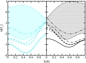
Figure 15: (Color online) Comparison of the hole dispersions and the continua formed by one triplon and one hole state for $x=1$, $x_{\square}=0$, $\lambda=2$. Left: The odd hole dispersion was derived from pc SCUT (cyan/gray solid), gs SCUT (cyan/gray dashed) and by exact diagonalization (cyan/gray dotted). The cyan (gray) shaded area depicts the continuum with one even hole and one triplon (derived from the same gs SCUT calculation). The cyan (gray) dash dot dot line is the lower boundary of the continuum formed by two triplons and one odd hole. Right: The even hole dispersion was derived from pc SCUT (black solid), gs SCUT (black dashed), by exact diagonalization (black dotted) and by series expansion (black dashed-dotted). The black shaded area depicts the continuum with one odd hole and one triplon (derived from the same gs SCUT calculation). The black dash dot dot line is the lower boundary of the continuum formed by two triplons and one even hole.

Let us consider the continua formed by one hole and one triplon. The continua consisting of one hole and one triplon are compared to the one-hole dispersions in Fig. 15. The continua do not overlap with the hole dispersions, but they are very close to them. The only exception is the series expansion result for the odd band which actually exhibits an overlap with the continuum formed by a triplon and an even hole state.

Figure 16: ROD for the SCUT for $x=1$, $x_{\square}=0$, $\lambda=2$ induced by the pc generator (solid line) and by the gs generator (dashed line).

The behavior of the ROD yields further evidence why the gs results should be preferred to the pc results for this parameter regime. Fig. 16 depicts the evolution of the ROD during the flow for both generators. Not only that the pc SCUT converges extremely slowly, the shape of the curve for $lJ_{\perp}<100$ is an indicator for a problem with respect to the sorting of the eigenenergies. It is a generic behavior of the ROD that the sorting of the eigen values (cf. Eq. (11)) is reflected by features for small values of $l$. When the sorting is completed the ROD decreases exponentially with a constant rate. For the gs generator the decrease of the ROD attains this rate not later than at $lJ_{\perp}=5$. Before this point the decrease is slower . The kink of the gs ROD at $lJ_{\perp}\approx 110$ with the subsequent upturn is again most probably due to cumulating numerical inaccuracies. This is no real problem because the gs ROD has already fallen below a value of less than $10^{-16}$ at $lJ_{\perp}\approx 110$ and can hence be neglected. However, the pc ROD exhibits several humps and a pronounced rise at $lJ_{\perp}=34$ before a decrease with a constant rate is achieved. This is a typical indication for a suppressed divergence that would actually occur for a less strict truncation. If such a behavior occurs the transformation is susceptible to truncation errors. The physical origin of these problems is the strong overlap between the one-hole-one-triplon continuua and the one-hole-two-triplon continua (see Fig. 15).

IV.2 Calculations with Restricted Generators

Results from exact diagonalization are available for $x=1$ and $\lambda=3$, but even the gs generator does not induce convergence for this case. However, if we apply the generator restriction introduced in Sect. III.2 to the gs generator, it yields convergence for $\Delta n_{\mathrm{max}}\leqslant 2$. Then some coupling between one hole and one hole plus one triplon $1\text{h}\to 1\text{h}+1\text{t}$ is not eliminated completely. Because the Hamiltonian is not diagonalised with respect to the terms omitted from the generator, the hole dispersions we obtain from a Fourier transformation are only upper limits for the actual result. But this is a minor problem since the remaining matrix elements are small. Another way of improvement (not followed here) would be to use self-consistent Born approximation to deal with the remaining coupling $1\text{h}\to 1\text{h}+1\text{t}$.

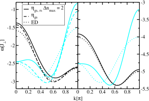
Figure 17: (Color online) Comparison of the one-hole dispersions from the restricted generator with the gs and the exact diagonalization results. Left panel: $x=1$, $x_{\square}=0$, $\lambda=2$. Right panel: $x=1$, $x_{\square}=0$, $\lambda=3$. The black lines represent the even hole dispersion and the cyan (gray) lines represent the odd hole dispersion.

Here we compare the results for upper limits from the restricted generator for $x=1$ and $\lambda=2$ with the gs results before we investigate the results for $x=1$ and $\lambda=3$. The left panel of Fig. 17 shows the comparison of the one-hole dispersions for $x=1$ and $\lambda=2$. We see that for $\Delta n_{\mathrm{max}}\leqslant 2$ the upper boundary from the restricted gs generator is close to the result from the full gs generator. In the right panel of Fig. 17 the results from the restricted gs generator are compared to the exact diagonalization results for $x=1$ and $\lambda=3$. For the even hole dispersion the agreement between the result from the restricted gs generator and the exact diagonalization result is almost perfect. Also the agreement for the odd hole dispersion is good. The deviations are comparable to the deviations of the result by the full gs generator from the exact diagonalization result for $x=1$ and $\lambda=2$.

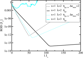
Figure 18: (Color online) ROD for the SCUT calculated with the full gs generator and with the restricted gs generator for different parameters.

The investigation of the ROD shows that the restricted gs generator yields a faster convergence than the full gs generator for $x=1$ and $\lambda=2$ (see Fig. 18). For $x=1$ and $\lambda=3$ the ROD diverges for the full generator, while the restricted generator induces convergence (see also Fig. 18). Note that the kinks of the RODs in Fig. 18 with an increase afterwards are again probably due to a feedback of numerical inaccuracies. But all the kinks appear at values where the ROD is already smaller than $10^{-12}$. So the flow can be considered to be converged at the kinks for practical purposes.

The terms left out from the restricted generator still contribute to the Hamiltonian after the transformation. These contributions yield an estimate of the difference between the actual energy and the upper boundary for the energy resulting from the restricted generator. For the $432$ terms of the form $a^{\dagger}_{\tau,\sigma,n}t^{\dagger}_{\alpha,n+\Delta n}a^{\phantom{\dagger}}_{\tau^{\prime},\sigma^{\prime},m}$ or $a^{\dagger}_{\tau,\sigma,m}t^{\phantom{\dagger}}_{\alpha,n}a^{\phantom{\dagger}}_{\tau^{\prime},\sigma^{\prime},n+\Delta n}$ the sum over their squared coefficients is $\approx 0.48\,\mathrm{J}_{\perp}^{2}$; its square root yields $\approx 0.16\,\mathrm{J}_{\perp}$.

Figure 19: (Color online) Comparison of gs SCUT (solid lines) and exact diagonalization for various finite ladders with $L$ rungs (discrete points) for $x=1$, $\lambda=1$. The lower boundaries of the continua calculated by gs SCUT are shown as dashed lines. The results for the even hole state are black, the results for the odd hole state are cyan (gray).

To understand the deviations between SCUT and exact diagonalization we also compare our results to the complete spectrum from exact diagonalization. In Fig. 19 the results of the exact diagonalization for various finite ladders with $L$ rungs are compared to the results from the gs generator for $x=1$ and $\lambda=1$. For the even band the lowest lying eigen value can be clearly distinguished from the larger eigen values, which are the precursor of the continuum. This holds true for all momenta. In the case of the odd band the lowest eigen value is very close to the higher ones for large momenta. Our calculation of the continuum predicts that the dispersion merges with the continuum in this region. Also the quantum Monte Carlo result for the spectral weight Brunner et al. (2001) exhibits no peak below the continuum around $k\approx\pi$.

Our result for the even band is in excellent agreement with the exact diagonalization result. Around $k\approx 0.25\pi$ our result for the odd band lies above the exact diagonalization result while it lies below the exact diagonalization result around $k\approx 0.6\pi$.

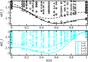
Figure 20: (Color online) Comparison of gs SCUT (solid lines) and exact diagonalization for various finite ladders with $L$ rungs (discrete points) for $x=1$, $\lambda=2$. The lower boundaries of the continua calculated by gs SCUT are shown as dashed lines. The results for the even hole state are black, the results for the odd hole state are cyan (gray).

In Fig. 20 we compare the results of the exact diagonalization with the results from the gs generator for $x=1$ and $\lambda=2$. For the even band for large momenta the lowest lying eigen value is clearly distinguishable from the larger eigen values, which are again the precursor of the continuum. The same is true for the odd band for small momenta. But for small momenta in case of the even band and for large momenta in case of the odd band the lowest eigen value is very close to the higher ones. Hence the distinction between hole dispersion and continuum becomes difficult in these regions. It is even questionable if they are actually distinct or if the dispersion merges with the continuum. In these regions the deviations between SCUT and exact diagonalization are the largest. We conclude that the SCUT suffers from truncation errors if the dispersion runs close to continua or even enters them. Also the lower boundary of the continuum that we calculated from the gs result is higher at $k=0$ for the even band and at $k=\pi$ for the odd band than we would expect from the exact diagonalization data.

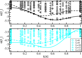
Figure 21: (Color online) Comparison of SCUT from the restricted gs generator with $\Delta n_{\mathrm{max}}=2$ (solid lines) and exact diagonalization for various numbers or rungs $L$ (symbols) for $x=1$, $\lambda=3$. The dashed lines are estimates for the lower boundaries of the continua based on the result from the restricted gs generator. The results for the even hole state are black, the results for the odd hole state are cyan (gray).

For $x=1$ and $\lambda=3$ the exact diagonalization results are shown in Fig. 21 for various finite ladders with $L$ rungs. The odd hole dispersion is more difficult to distinguish from the continuum than for $x=1$ and $\lambda=2$. Also for small momenta the lowest eigen value is very close to the higher ones. The hole dispersions from the restricted gs generator with $\Delta n_{\mathrm{max}}=2$ is also depicted in Fig. 21. In the region $0.5\pi\lesssim k\lesssim 0.8\pi$ this dispersion lies below the exact diagonalization data.

V Hole Dispersions with Ring Exchange

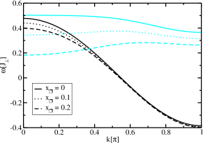
Figure 22: (Color online) One-hole dispersions with even parity (black) and odd parity (cyan/gray) for $x=0$, $\lambda_{\perp}=\lambda_{\parallel}=0.5$ and various values for $x_{\square}$.

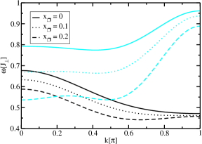
Figure 23: (Color online) One-hole dispersions with even parity (black) and odd parity (cyan/gray) for $x=0.5$, $\lambda_{\perp}=\lambda_{\parallel}=0.25$ and various values for $x_{\square}$.

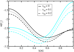
Figure 24: (Color online) One-hole dispersions with even parity (black) and odd parity (cyan/gray) for $x=1$, $\lambda_{\perp}=\lambda_{\parallel}=2$ and various values for $x_{\square}$.

Since the ring exchange is needed for an adequate description of the experimentally available systems, we also investigate the influence of the ring exchange on the doped ladder, see Ref. Schmidt and Uhrig, 2005 and references therein. A typical value is $x_{\square}\approx 0.2$ Nunner et al. (2002); Schmidt and Uhrig (2005). As for the examination of the anisotropic hopping we take the reliable results for $x=0$, $\lambda_{\perp}=\lambda_{\parallel}=0.5$; $x=0.5$, $\lambda_{\perp}=\lambda_{\parallel}=0.25$ and $x=1$, $\lambda_{\perp}=\lambda_{\parallel}=2$ without ring exchange as starting point for our investigation.

For the first case $x=0$, $\lambda_{\perp}=\lambda_{\parallel}=0.5$ the influence of the ring exchange is the weakest (see Fig. 22). The odd band hardly changes. It is slightly lowered – only the maximum is decreased more strongly. For the even band, however, the changes are more pronounced. It is strongly lowered so that a band crossing occurs and the shape changes. A local miminum appears at $k=0$ developing into the global minimum with growing $x_{\square}$.

Fig. 23 depicts the case $x=0.5$, $\lambda_{\perp}=\lambda_{\parallel}=0.25$. Both bands are lowered stronger for small $k$ than for large $k$. Also the shape of both bands changes. While the minimum of the even band moves to $k\approx 0.65\pi$ for $x_{\square}=0.2$ and a local maximum occurs at $k=\pi$, the local maximum at $k=0$ of the odd band moves to $k\approx 0.55\pi$ and a local minimum at occurs $k=0$.

For $\lambda_{\perp}=\lambda_{\parallel}=2$ and $x=1$ only the gs results are discussed because the pc generator yields no conclusive results for these parameters without ring exchange. The resulting one-hole dispersions are shown in Fig. 24. The increase of $x_{\square}$ yields a lowered dispersion for both bands. The shape of the bands is conserved, but for the odd band the decrease is pronounced around $k=\pi$. Even an increase of the energy can be observed for the even band around $k=\pi$.

VI Summary

The aim of the present paper was to establish an approach for doped low-dimensional quantum antiferromagnets which yields an effective model for the motion of charges. To this end, we employed a self-similar continuous unitary transformation (SCUT) to lightly doped spin ladders. The method is particularly suited to provide effective models beyond numerical results for special quantities. Spin ladders are a particularly well suited system because their magnetic excitations are very well understood Schmidt and Uhrig (2005); Bouillot et al. (2011).

We are able to calculate the one-hole dispersions by means of SCUT. The agreement with results from series expansion is very good for small parameters. Even in the regime $x=1$, $x_{\square}=0$, $2<\lambda<3$ the agreement with the exact diagonalisation results is still very good for the even band and satisfactory for the odd one. The hole dispersions are strongly influenced by the triplons. Because the one-hole dispersion with odd parity has a larger local energy which is influenced more strongly by the higher lying continuum, it changes more explicitly with increasing hopping constants. Therefore the deviations from the simple cosine shape are more pronounced for the odd band. These deviations grow if either the magnetic coupling or the strength of the hopping is increased:

• The broadening of the odd band is slowing down, then turning into a narrowing. Finally the shape changes completely under the influence of the second harmonic so that the maximum at $k=0$ is only local, the total maximum occurs at $k=\pi$ and the minimum lies between $0$ and $\pi$.

• The shift upwards is also slowing down and then turning into a shift downwards due to the influence of the continuum formed by one triplon and one even hole state. In the regime around $x=1$ and $\lambda_{\perp}=\lambda_{\parallel}=2$ the average odd dispersion is approximately as low as the average even dispersion.

For the even band the deviations from the cosine shaped dispersion consist essentially in the growth of the second harmonic. For $x=1$ and $\lambda_{\perp}=\lambda_{\parallel}=2$ the minimum moves from $k=\pi$ into the region $k\approx\frac{\pi}{2}$. A local maximum at $k=\pi$ occurs. But the absolute maximum remains at $k=0$.

The combination of these effects for $x=1$ and $\lambda_{\perp}=\lambda_{\parallel}=2$ yields a crossing of the two dispersions. The crossing point lies between the minima of the bands. However, the pc generator is not applicable for the SCUT if the parameters are in this region. This is suggested by the deviations from the series expansion and from exact diagonalisation as well as by the peculiar convergence behavior of the SCUT.

In the regime $x\approx 1$ and $\lambda_{\perp}=\lambda_{\parallel}\gtrsim 1$ the pc generator is no longer suitable because the convergence of the flow is hindered by the overlap between the one-hole-one-triplon continuua and the one-hole-two-triplon continua. The pc results deviate from the series expansion and exact diagonalisation results. Furthermore the convergence is very slow and exhibits features that indicate problems in the sorting of the eigen values.

The remedy is to use the gs generator which only decouples the zero-triplon subspace from the remaining Hilbert space. Then the hole dispersions are similar to the exact diagonalisation results. Although there are small deviations from the series expansion, the agreement is astonishingly good. Because the exact diagonalisation studies a ladder with fourteen rungs, finite size effects are present so that a part of the deviations stem from them. The remaining deviations are probably due to truncation errors . Another aspect in favour of the gs generator is the satisfactory convergence behavior.

The treatment of the case $\lambda_{\perp}=\lambda_{\parallel}>2$ is problematic even for the gs generator because the convergence is hindered by the overlap between the odd one-hole dispersion and the continuum formed by one even hole and one triplon. To achieve convergence in this regime we have developed the following restriction for the gs generator. A term affecting the hole-triplon continuum is omitted, if the distance between the triplon and the hole state on which the term acts is larger than $\Delta n_{\mathrm{max}}$. Strictly, the effective Hamiltonian yields an upper boundary for the hole dispersions. The comparison of the results from the full gs generator and from the restricted gs generator for $x=1$ and $\lambda_{\perp}=\lambda_{\parallel}=2$ shows that the upper boundary given by the result from the restricted generator is already very close to the result from the full generator for $\Delta n_{\mathrm{max}}=2$. For $x=1$ and $\lambda_{\perp}=\lambda_{\parallel}=3$ this restriction induces convergence, while the flow diverges for $\Delta n_{\mathrm{max}}>2$. The estimates we obtain for the hole dispersions agree again well with the exact diagonalisation results.

If $x=1,x_{\square}=0$ and $\lambda=\lambda_{\perp}=\lambda_{\parallel}=3$ or $\lambda=\lambda_{\perp}=\lambda_{\parallel}=2$ the bands exhibit a similar shape and relative position to each other so that still a crossing at $k\approx 0.5\pi$ occurs. But the energy is lowered and the bandwith of both bands is increased by a factor of $\approx 1.5$ if $\lambda$ is changed from 2 to 3. The results from the restricted gs generator yield an estimate for the even band which is in good agreement with the exact diagonalisation result, while the odd hole dispersion exhibits deviations that are very similar to the deviations between the exact diagonalisation and the full gs generator for $\lambda_{\perp}=\lambda_{\parallel}=2$.

The case $x=\lambda_{\perp}=\lambda_{\parallel}=0.5$ is a special one. Both the pc and the gs generator (even with increased maximal extensions) exhibit deviations from the series expansion results for the odd hole state. These deviations stem apparently from the closeness (or even overlap) of the continuum formed by one even hole and one triplon. If the lowering of the odd band is overestimated by the SCUT or underestimated by the series expansion is not clear.

The ring exchange leads to a lowering of the hole dispersions. This effect is least pronounced for the even band around $k=\pi$. The deformation of the band shape is most pronounced for the odd band.

Summarizing, the essential achievement of this paper is the development of a unitary transformation which allows us to disentangle the motion of the doped charges, the holes, and the magnetic excitations, triplons. Thereby an effective model for the motion of the holes and the triplons has been derived. The challenge was to systematically derive this effective model even in the experimentally relevant regime $\lambda\approx 3$ where the hopping takes about three times the value of the magnetic exchange constants. This challenge could only be met by modification of the unitary transformation in the spirit of what was done in Ref. Fischer et al., 2010.

VII Outlook

Ladders doped with more than one hole have not yet been treated by the SCUT. To do so the approach presented here has to be extended to include also interaction terms between two holes. This step will be subject of future research because it will address the key question how large the attractive forces between two doped charges are. In view of the Cooper pair formation in doped cuprate superconductors this is a very interesting issue. Of course, numerical and diagrammatic results for bound states of two holes exist White and Scalapino (1997); Jeckelmann et al. (1998); Jurecka and Brenig (2002); Roux et al. (2005). But so far no effective model has been derived which incorporates the attractive potential explicitly.

The fact that we could realize a systematic mapping of the initial doped spin ladder to an effective model for the motion of single excitations is encouraging for the next step incorporating the hole-hole interaction. The additionally required resources, for instance the increase in the number of coefficients, are significant. We estimate that about six times more terms have to be kept track of. Still this should be realizable in the near future.

We expect that a substantial gain in the understanding of Cooper pair formation and thus of superconductivity in doped Mott insulators will be possible.

Appendix A Finite Size Scaling of the Exact Diagonalisation Results

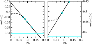
Figure 25: (Color online) Finite size scaling of the exact diagonalization results for $x=1$ $\lambda=1$ in case of the odd band at $k=0$ and at $k=0.5\pi$. The cyan (gray) circles depict the exact diagonalization results for finite ladders with various numbers of rungs $L$. The solid black line is a linear extrapolation with respect to $\frac{1}{L}$ and the dashed line is an extrapolation based on exponential saturation (see Eq. (16)). For comparison the result from the gs SCUT is also shown (solid cyan/gray).

To understand the deviations between SCUT and exact diagonalization in case of the odd band we also study the finite size scaling of the exact diagonalization. First we consider the exact diagonalization results for $x=1$ and $\lambda=1$ shown in Fig. 19. Around $k\approx 0.25\pi$ our result for the odd band lies above the exact diagonalization result, while it lies below the exact diagonalization result around $k\approx 0.6\pi$.

An investigation of the finite size scaling for the exact diagonalization data in these regions is difficult because we have two points at most for an extrapolation. Thus we consider $k=0$, where an extrapolation is conclusive. The result of this extrapolation is used to support an extrapolation in the region where the deviations are observed. The left panel of Fig. 25 shows the finite size scaling for $k=0$ using two kinds of extrapolation. The first is a simple linear extrapolation with respect to $\frac{1}{L}$, while the second assumes an exponential saturation with increasing $L$ so that

$$\Delta\omega\propto\mathrm{e}^{-\frac{L}{\xi}}$$ (16)

holds true for the difference $\Delta\omega$ from the limit for $L\rightarrow\infty$. The correlation length $\xi$ is determined to be $\approx 4.32$ by this extrapolation. The correlation length can be used to apply the second extrapolation also for $k=0.5\pi$ where only two results are obtained by exact diagonalization.

The finite size scaling for $k=0.5\pi$ in case of the odd band is investigated by both extrapolations in the right panel of Fig. 25. The extraploation results at $k=0$ are still close to the gs SCUT result and the extrapolation results at $k=0.5\pi$ are in good agreement with the gs SCUT result. The linear extrapolation is even in excellent agreement with our result. Note that the points from the $L=6$ calculation are omitted for the extrapolations because they deviate from the behavior of the other points due to the very small size.

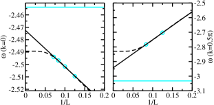
Figure 26: (Color online) Finite size scaling of the exact diagonalization results for $x=1$ $\lambda=2$ in case of the odd band at $k=0$ and at $k=0.5\pi$. The cyan (gray) circles depict the exact diagonalization results for finite ladders with various numbers of rungs $L$. The solid black line is a linear extrapolation with respect to $\frac{1}{L}$ and the dashed line is an extrapolation based on exponential saturation (see Eq. (16)). For comparison the result from the gs SCUT is also shown (solid cyan/gray).

For $x=1$ and $\lambda=2$ the SCUT result for the dispersions comes close to the extrapolation of exact diagonalization results in the regions where the continuum is distinguishable from the hole dispersion. This is most obvious for the odd band at $k=0$. The left panel of Fig. 26 shows the finite size scaling for this case using the same extrapolations like for $x=1$ and $\lambda=1$. We determine $\xi$ to be $\approx 4.03$ by the extrapolation based on exponential saturation. The correlation length is again used to apply this kind of extrapolation also for $k=0.5\pi$.

The finite size scaling for $k=0.5\pi$ in case of the odd band is investigated by both extrapolations in the right panel of Fig. 26. For both momenta the linear extrapolation comes close to the SCUT result, but also the extrapolation based on exponential saturation does not exhibit large deviations from the SCUT result. The deviation for $k=0$ is $\approx 2\%$ and the deviation for $k=0.5\pi$ is $\approx 7\%$. The points from the $L=6$ calculation are omitted for the extrapolations because they deviate from the behavior of the other points due to the small size of the system.

For $x=1$ and $\lambda=3$ the tendency of the finite size scaling at $k=0.5\pi$ indicates that the exact diagonalization results overestimate the energy of the odd band in this region so that one can expect that a proper finite size scaling yields a dispersion that lies completely below the upper boundary provided by the restricted SCUT energies.

However, an extrapolation from the two points ($L=8$ and $L=12$) at $k=0.5\pi$ is not conclusive. We have several points for an extrapolation for $k=0$ and $k=\pi$, but there the distinction between continuum and dispersion is difficult. Because the gs SCUT diverges without restriction of the generator, we actually expect that a strong overlap of the energies of single holes and of the energies of hole plus triplon states is present.

References

- Dagotto and Moreo (1988) E. Dagotto and A. Moreo, Phys. Rev. B 38, 5087 (1988).
- Dagotto et al. (1992) E. Dagotto, J. Riera, and D. Scalapino, Phys. Rev. B 45, 5744 (1992).
- Barnes et al. (1993) T. Barnes, E. Dagotto, J. Riera, and E. S. Swanson, Phys. Rev. B 47, 3196 (1993).
- Dagotto and Rice (1996) E. Dagotto and T. M. Rice, Science 271, 618 (1996).
- Troyer et al. (1996) M. Troyer, H. Tsunetsugu, and T. M. Rice, Phys. Rev. B 53, 251 (1996).
- White and Scalapino (1997) S. R. White and D. J. Scalapino, Phys. Rev. B 55, 6504 (1997).
- Jeckelmann et al. (1998) E. Jeckelmann, D. J. Scalapino, and S. R. White, Phys. Rev. B 58, 9492 (1998).
- Oitmaa et al. (1999) J. Oitmaa, C. J. Hamer, and Z. Weihong, Phys. Rev. B 60, 16364 (1999).
- Sushkov (1999) O. P. Sushkov, Phys. Rev. B 60, 14517 (1999).
- Johnston et al. (2000) D. C. Johnston, M. Troyer, S. Miyahara, D. Lidsky, K. Ueda, M. Azuma, Z. Hiroi, M. Takano, M. Isobe, Y. Ueda, et al., condmat/0001147 (2000).
- Brunner et al. (2001) M. Brunner, S. Capponi, F. F. Assaad, and A. Muramatsu, Phys. Rev. B 63, 180511 (2001).
- Jurecka and Brenig (2001) C. Jurecka and W. Brenig, Phys. Rev. B 63, 94409 (2001).
- Jurecka and Brenig (2002) C. Jurecka and W. Brenig, J. Low Temp. Phys. 126, 1165 (2002).
- Schmidt and Uhrig (2005) K. P. Schmidt and G. S. Uhrig, Mod. Phys. Lett. B 19, 1179 (2005).
- Roux et al. (2005) G. Roux, S. R. White, S. Capponi, A. Läuchli, and D. Poilblanc, Phys. Rev. B 72, 014523 (2005).
- Bouillot et al. (2011) P. Bouillot, C. Kollath, A. M. Läuchli, M. Zvonarev, B. Thielemann, C. Rüegg, E. Orignac, R. Citro, M. Klanjšek, C. Berthier, et al., Phys. Rev. B 83, 054407 (2011).
- Harris and Lange (1967) A. B. Harris and R. V. Lange, Phys. Rev. 157, 295 (1967).
- Zhang and Rice (1988) F. C. Zhang and T. M. Rice, Phys. Rev. B 37, 3759 (1988).
- Schmidt and Uhrig (2003) K. P. Schmidt and G. S. Uhrig, Phys. Rev. Lett. 90, 227204 (2003).
- Knetter et al. (2003) C. Knetter, K. P. Schmidt, and G. S. Uhrig, J. Phys. A: Math. Gen. 36, 7889 (2003).
- J. Oitmaa and Zheng (2006) C. H. J. Oitmaa and W. Zheng, Series Expansion Methods for Strongly Interacting Lattice Models (Cambridge University Press, Cambridge, UK, 2006).
- Fischer et al. (2010) T. Fischer, S. Duffe, and G. S. Uhrig, New J. Phys. 10, 033048 (2010).
- Vuletić et al. (2006) T. Vuletić, B. Korin-Hamzić, T. Ivek, S. Tomić, B. Gorshunov, M. Dressel, and J. Akimitsu, Phys. Rep. 428, 169 (2006).
- Uehara et al. (1996) M. Uehara, T. Nagata, J. Akimitsu, H. Takahashi, N. Môri, and K. Kinoshita, J. Phys. Soc. Jpn. 65, 2764 (1996).
- Gopalan et al. (1994) S. Gopalan, T. M. Rice, and M. Sigrist, Phys. Rev. B 49, 8901 (1994).
- Matsuda et al. (2000) M. Matsuda, K. Katsumata, R. S. Eccleston, S. Brehmer, and H.-J. Mikeska, Phys. Rev. B 62, 8903 (2000).
- Schmidt and Uhrig (2007) K. P. Schmidt and G. S. Uhrig, Phys. Rev. B 75, 224414 (2007).
- Anderson (1950) P. W. Anderson, Phys. Rev. 79, 350 (1950).
- Hamerla et al. (2010) S. A. Hamerla, S. Duffe, and G. S. Uhrig, Phys. Rev. B 82, 235117 (2010).
- Coldea et al. (2001) R. Coldea, S. M. Hayden, G. Aeppli, T. G. Perring, C. D. Frost, T. E. Mason, S. W. Cheong, and Z. Fisk, Phys. Rev. Lett. 86, 5377 (2001).
- Mizuno et al. (1999) Y. Mizuno, T. Tohyama, and S. Maekawa, J. Low Temp. Phys. 117, 389 (1999).
- Brehmer et al. (1999) S. Brehmer, H. Mikeska, M. Müller, N. Nagaosa, and S. Uchida, Phys. Rev. B 60, 329 (1999).
- Sachdev and Bhatt (1990) S. Sachdev and R. N. Bhatt, Phys. Rev. B 41, 9323 (1990).
- Duffe (2010) S. Duffe, Effective Hamiltonians for Undoped and Hole-Doped Antiferromagnetic Spin- Ladders by Self-Similar Continuous Unitary Transformations in Real Space (PhD Thesis, available at http://t1.physik.tu-dortmund.de/uhrig/phd.html, TU Dortmund, 2010).
- Głazek and Wilson (1993) S. D. Głazek and K. G. Wilson, Phys. Rev. D 48, 5863 (1993).
- Wegner (1994) F. J. Wegner, Ann. Physik 3, 77 (1994).
- Kehrein (2006) S. Kehrein, The Flow Equatin Approach to Many-Particle Systems, vol. 217 of Springer Tracts in Modern Physics (Springer, Berlin, 2006).
- Mielke (1997) A. Mielke, Ann. Physik 6, 215 (1997).
- Reischl et al. (2004) A. Reischl, E. Müller-Hartmann, and G. S. Uhrig, Phys. Rev. B 70, 245124 (2004).
- Uhrig and Schulz (1996) G. S. Uhrig and H. J. Schulz, Phys. Rev. B 54, 9624(R) (1996).
- Trebst et al. (2000) S. Trebst, H. Monien, C. J. Hamer, Z. Weihong, and R. Singh, Phys. Rev. Lett. 85, 4373 (2000).
- Knetter et al. (2001) C. Knetter, K. P. Schmidt, M. Grüninger, and G. S. Uhrig, Phys. Rev. Lett. 87, 167204 (2001).
- Mielke (1998) A. Mielke, Eur. Phys. J. B 5, 605 (1998).
- Uhrig and Normand (1998) G. S. Uhrig and B. Normand, Phys. Rev. B 58, R14705 (1998).
- Knetter and Uhrig (2000) C. Knetter and G. S. Uhrig, Eur. Phys. J. B 13, 209 (2000).
- Dusuel and Uhrig (2004) S. Dusuel and G. S. Uhrig, J. Phys. A: Math. Gen. 37, 9275 (2004).
- Nunner et al. (2002) T. S. Nunner, P. Brune, T. Kopp, M. Windt, and M. Grüninger, Phys. Rev. B 66, 180404(R) (2002).