A template of atmospheric $O_{2}$ circularly polarized emission for CMB experiments

Abstract

We compute the circularly polarized signal from atmospheric molecular oxygen. Polarization of $O_{2}$ rotational lines is caused by Zeeman effect in the Earth magnetic field. We evaluate the circularly polarized emission for various sites suitable for CMB measurements: South Pole and Dome C (Antarctica), Atacama (Chile) and Testa Grigia (Italy). An analysis of the polarized signal is presented and discussed in the framework of future CMB polarization experiments. We find a typical circularly polarized signal ($V$ Stokes parameter) of $\sim 50-300\ \mu$K at 90 GHz looking at the zenith. Among the other sites Atacama shows the lower polarized signal at the zenith. We present maps of this signal for the various sites and show typical elevation and azimuth scans. We find that Dome C presents the lowest gradient in polarized temperature: $\sim 0.3\ \mu$K$/^{\circ}$ at 90 GHz. We also study the frequency bands of observation: around $\nu\simeq 100$ GHz and $\nu\simeq 160$ GHz we find the best conditions because the polarized signal vanishes. Finally we evaluate the accuracy of the templates and the signal variability in relation with the knowledge and the variability of the Earth magnetic field and the atmospheric parameters.

1 Introduction

The observation of the Cosmic Microwave Background (CMB) from the ground can be performed inside the atmospheric windows, far from the main emission lines of the most abundant molecules. For the experiments devoted to the measurement of the polarization properties of the CMB it is mandatory to evaluate, in addition, the effects of the atmosphere. In a recent paper (Pietranera et al., 2007) the effects of ice crystal clouds in the upper troposphere have been considered, but the major effect arises from the polarized emission of the $O_{2}$ molecule. The relevance of this effect for CMB measurements has been pointed out by Hanany & Rosenkranz (2003), where for the first time a quantitative evaluation of the polarized signals has been presented. Also Keating et al. (1998) discuss the relevance of the polarized emission of the $O_{2}$ as a foreground for CMB observations.

Here we compute the polarized emission of the $O_{2}$ molecule, developing the formalism introduced in the pioneering works by Lenoir (1967, 1968). The interaction of the Earth magnetic field with the magnetic dipole moment of the atmospheric $O_{2}$ molecule induces Zeeman splitting onto the roto-vibrational lines. As a result of this interaction, radiation becomes weakly circularly polarized with a degree of polarization $\sim 10^{-4}-10^{-5}$. A linear polarization is also generated, but the signal is three or four orders of magnitude lower and still below the current detection sensitivity.

This circularly polarized signal can be considered a contaminant for CMB ground-based experiments for two reasons. The first one is that non-idealities in the instrument can produce conversion from circular to linear polarization: this leakage from the $V$ Stokes’ parameter to $\{Q,U\}$ can be the source of a spurious signal if the circularly polarized radiation of atmospheric oxygen is picked-up by the instrument. Here the effect on the recovery of the cosmological polarized signal is evident since CMB is expected to be only (weakly) linearly polarized (Hu & White, 1997).

The second one is that there is an increasing theoretical effort dedicated to the physical mechanisms able to create a non vanishing CMB circular polarization. In fact, there are several attempts to add terms to the standard electromagnetic lagrangian density, and to predict observable effects arising from these extensions. Among others, and without sake of completeness, we recall: test of the Shiff conjecture on the EEP (Carroll & Field, 1991); coupling between photons and slowly varying pseudoscalar fields (Harari & Sikivie, 1992), (Carlson & Garretson, 1994) and (Finelli & Galaverni, 2009); coupling between photons and pseudoscalar fields in presence of intergalactic magnetic fields (Agarwal et al., 2008); coupling between photons and vector fields to test Lorentz-invariance violating processes (Alexander et al., 2009). Authors, in all of these cases, show how a fundamental process induces optical activity in the Intergalactic Medium. In fact, the extensions of the standard lagrangian generate new terms in Maxwell’s equations (see eq. 3 in Harari & Sikivie (1992)), therefore leading to modified dispersion relations. We have to mention also the possibility of having a $V$-mode induced by last-scattering in a magnetized primordial plasma (see Giovannini (2009, 2010)) and, after recombination, by intergalactic magnetic fields through Faraday conversion (Cooray et al., 2003).

It is likely that, with increasing theoretical motivations, a dedicated experiment will be proposed in the near future to update the very early upper limits obtained by Lubin et al. (1983) and Partridge et al. (1988). The present work has been prepared also in this spirit.

In section 2 the basic physics of the process is presented, while in section 3 the tensor radiative transfer approach used to compute the atmospheric integrated signal is described. The analysis is applied to different sites: Dome C (Antarctica), South Pole, Atacama (Chile), Testa Grigia (Italian Alps), where mm-wave instruments are located. Results are reported in section 4. We compare the effect in different places and define the optimal observation bands in order to minimize the effect from this contaminant.

2 Polarized signal theory

$O_{2}$ is the only abundant atmospheric molecule with non-zero magnetic dipole moment, because the two electrons in the highest energy state couple with parallel spin. The presence of polarized radiation in the atmosphere is associated with the interaction of the magnetic dipole moment of the $O_{2}$ molecule and the Earth magnetic field. In the millimeter wave region of the electromagnetic spectrum, $O_{2}$ molecule presents a set of lines due to roto-vibrational transitions. The presence of the Earth magnetic field induces Zeeman splitting on these lines, which then become polarized.

Because of the Zeeman effect a quantum state represented by the quantum number $J$ is split in $2J+1$ states, each of them described by a different value of $M_{J}$, under the condition $|M_{J}|\leq J$. The selection rules permit the following transitions, $\Delta J=+1$ (called $L^{+}$) and $\Delta J=-1$ (called $L^{-}$):

$$\begin{array}[]{llllll}&\Delta J=+1\ :&\ J=L&\ \rightarrow&\ J=L+1&\ \ (L^{+})\\ &\Delta J=-1\ :&\ J=L&\ \rightarrow&\ J=L-1&\ \ (L^{-})\end{array}$$

Under these conditions, selection rules permit to have $\Delta M_{J}=0$ ($\pi$ transitions) and $\Delta M_{J}=\pm 1$ ($\sigma_{\pm}$ transitions). In Table 1 we report the frequencies of $O_{2}$ roto-vibrational transitions allowed by the Fermi Golden Rule and used for our calculation, together with their corresponding quantum number ($L^{\pm}$). We stop to $L^{\pm}=37$ because of lack of information about the line broadening and mixing parameters (see Liebe et al. (1992)) of higher orders. We also verified the effect of adding lines with $L^{\pm}>37$: far from the transition frequencies the difference is negligible ($\Delta V$/$V<10^{-5}$).

Table 1: Line frequency and corresponding quantum number $L^{\pm}$ used for the computation of the atmospheric $O_{2}$ polarized signal.

$L^{\pm}$	$\nu_{t}(L^{-})$  (GHz)	$\nu_{t}(L^{+})$  (GHz)
1	118.750343	56.264777
3	62.486255	58.446580
5	60.306044	59.590978
7	59.164215	60.434776
9	58.323885	61.150570
11	57.612480	61.800155
13	56.968180	62.411223
15	56.363393	62.997977
17	55.783819	63.568520
19	55.221372	64.127777
21	54.671145	64.678898
23	54.130002	65.224065
25	53.595751	65.764744
27	53.066908	66.302082
29	52.542392	66.836820
31	52.021405	67.369589
33	51.503339	67.900867
35	50.987728	68.431005
37	50.474204	68.960312

Radiation intensity and polarization direction are also determined by the angle ($\theta$) between the line of sight and the Earth magnetic field. We must define a reference system onto which the vector $\mn@boldsymbol{E}$ of the electromagnetic wave is projected. A good choice is the 3D geomagnetic system (see Lenoir (1968)) centered at the geographic Earth center: $z$ axis correspondes to the geomagnetic dipole axis and angles $\psi_{m}$ and $\phi_{m}$ identify the geomagnetic latitude and longitude respectively. Matrix representing the polarized intensity I can be evaluated through the coherence matrix ($\mn@boldsymbol{\rho}$) for the different transitions:

$$\textbf{I}_{\Delta M_{J}}(S,L,M_{J})=P_{trans,\Delta M_{J}}(S,L,M_{J})\ \mn@boldsymbol{\rho}_{\Delta M_{J}},$$

In this reference frame the matrices for the three different transitions become:

$$\Delta M_{J}=-1\ :\ \ \ \ \mn@boldsymbol{\rho}_{\sigma_{-}}=\left(\begin{array}[]{cc}1&i\cos\theta\\ -i\cos\theta&\cos^{2}\theta\\ \end{array}\right)$$ (5)

$$\Delta M_{J}=+1\ :\ \ \ \ \mn@boldsymbol{\rho}_{\sigma_{+}}=\left(\begin{array}[]{cc}1&-i\cos\theta\\ i\cos\theta&\cos^{2}\theta\\ \end{array}\right)$$ (8)

$$\Delta M_{J}=0\ :\ \ \ \ \ \ \mn@boldsymbol{\rho}_{\pi}\ \ =\left(\begin{array}[]{cc}0&0\\ 0&\sin^{2}\theta\\ \end{array}\right),$$ (11)

where $P_{trans}$ denotes the transition probability for the line identified by the quantum numbers $(S,L,J,M_{J})$ and fix their relative intensity. Equations (5) - (11) show that $\sigma_{-}$ and $\sigma_{+}$ lines produce circular polarization, due to the off-diagonal terms in the matrices. Besides the combination of the three transitions generate also a small fraction of linear polarization.

The total coherence matrix $\textbf{{A}}_{tot}$ can be derived by expressing the whole contribution given by the superposition of the different lines:

$$\textbf{{A}}_{tot}=\!C(\nu,P,T)\!\!\!\!\sum_{\Delta M_{J}=-1}^{\Delta M_{J}=+1}\!\!\!\mn@boldsymbol{\rho}_{\Delta M_{J}}\!\!\!\!\!\!\sum_{M_{J}=-J}^{+J}\!\!\!\!\!\!\!\!P_{trans}(S,L,M_{J},\Delta J,\Delta M_{J})$$

$$F(\nu,\nu_{k},\Delta\nu_{c}).$$

I matrices are multiplied by two weight factors: the first one, $C(\nu,P,T)$, takes into account the dependence on pressure, temperature and frequency (Lenoir, 1968):

$$C(\nu,T,P)=0.229\frac{P\nu^{2}}{T^{3}}e^{\frac{-E_{L}}{K_{B}T}};$$ (12)

the second function, $F(\nu,\nu_{k},\Delta\nu_{c})$, is the line profile. We neglect the Doppler effect and consider only the collisional line broadening, which is dominant in the lower layers of the atmosphere where most of the signal is generated. Therefore we use the collisional line profile (Van Vleck & Weisskopf, 1945) corrected for the line mixing effects as shown by Rosenkranz & Staelin (1988) and Liebe et al. (1992). The line profile used is then:

$$F(\nu,\nu_{k},\Delta\nu_{c})=F_{\Delta}-F_{Y}$$ (13)

where:

$$F_{\Delta}=\Delta\nu_{c}\left[\frac{1}{(\nu_{k}-\nu)^{2}+\Delta\nu_{c}^{2}}+\frac{1}{(\nu_{k}+\nu)^{2}+\Delta\nu_{c}^{2}}\right]$$

$$F_{Y}=Y_{k}\left[\frac{\nu_{k}-\nu}{(\nu_{k}-\nu)^{2}+\Delta\nu_{c}^{2}}+\frac{\nu_{k}+\nu}{(\nu_{k}+\nu)^{2}+\Delta\nu_{c}^{2}}\right]\ .$$

Here the line broadening is:

$$\Delta\nu_{c}=A_{0}\ P\left(\frac{300}{T}\right)^{0.8}$$ (14)

and the line mixing coefficient is:

$$Y_{k}=\left(A_{1}+A_{2}\frac{300}{T}\right)P\left(\frac{300}{T}\right)^{0.8}\ .$$ (15)

Here the coefficients $A_{0}$, $A_{1}$ and $A_{2}$, for each transition, are given in table 2 of Liebe et al. (1992), where calculations are compared with measurements. In eq. 13 $\nu_{k}=\nu_{t}+\delta_{\Delta M_{J}}$, where $\nu_{t}$ is the transition frequency, shown in table 1 and $\delta_{\Delta M_{J}}$ is a Zeeman induced frequency shift (Lenoir, 1968) given a magnetic field $\mn@boldsymbol{B}$ (nT):

$$\delta_{\Delta M_{J}}(MHz)=\left\{\begin{array}[]{ll}\frac{K_{0}B}{L+1}\left(\Delta M_{J}+M_{J}\displaystyle\frac{L-1}{L}\right)&\ \ (L^{+})\\ -\frac{K_{0}B}{L}\left(\Delta M_{J}+M_{J}\displaystyle\frac{L+2}{L+1}\right)&\ \ (L^{-})\end{array}\right.$$

Here $K_{0}=2.8026\times 10^{-5}$ and $\Delta M_{J}=0,\pm 1$. Taking into account all these relations and summarizing them, the total coherence matrix can be written as:

$$\textbf{{A}}_{tot}=a\mn@boldsymbol{\rho}_{\sigma_{-}}+b\mn@boldsymbol{\rho}_{\sigma_{+}}+c\mn@boldsymbol{\rho}_{\pi}=$$

$$\left(\begin{array}[]{cc}a+b&i(a-b)\cos\theta\\ -i(a-b)\cos\theta&(a+b)\cos^{2}\theta+c\sin^{2}\theta\\ \end{array}\right)=$$ (18)

$$\left(\begin{array}[]{cc}\alpha&i\beta\\ -i\beta&\gamma\end{array}\right)$$ (21)

This matrix expresses the coherence (polarization) properties of the signal coming from the Zeeman split $O_{2}$ lines. We get a matrix for a given atmospheric condition of pressure, temperature and height. In particular we notice that: 1) off-diagonal terms are non vanishing and conjugate purely imaginary complex numbers thus radiation is only circularly polarized ($V\neq 0$) since $U$ parameter is null; 2) circular polarization is larger when the line of sight is aligned with the Earth magnetic field: $V\propto\beta=(a-b)\cos\theta$; 3) the diagonal terms are still different ($\alpha\simeq\gamma$), so that Stokes’ parameter $Q\propto\alpha-\gamma\neq 0$; 4) linear polarization is larger when the line of sight is orthogonal to the Earth magnetic field: $Q\propto(a+b-c)\sin^{2}\theta$; 5) the component of non vanishing linear polarization ($Q$ parameter) is nearly aligned with the Earth magnetic field, even if a small Faraday rotation may occur (see Rosenkranz & Staelin (1988)). Actually it can be seen that the ratio of linear ($Q$) to circular ($V$) polarization is $Q/V\sim 10^{-4}$ (see Hanany & Rosenkranz (2003)). In the present paper we evaluate only the circularly polarized signal, as the linearly polarized one is still below the sensitivity of the current experiments (see section 4).

3 Coherence brightness temperature

3.1 Modeling the atmosphere

The propagation of radiation emitted by Oxygen molecules throughout atmosphere modifies its polarization properties. We compute the A matrix via a tensor radiative transfer approach. We compute the total coherence matrix in terms of brightness temperature and divide the atmosphere in $N$ layers of thickness $\Delta z=0.2$ km. We interpolate the atmospheric parameters profiles available in literature to fit this thickness. Than we take the average value of the physical parameters inside each layer and use the theory of radiative transfer, described in Lenoir (1968), to compute the signal emerging from one layer, taking into account all the layers lying above it:

$$\textbf{{T}}_{B}(z,\nu)=\sum_{i=1}^{N}\textbf{{WF}}(\Delta z_{i},\nu)T_{i}.$$ (22)

WF is a weight function for the physical temperature $T_{i}$ of the $i$-th layer, in which all the information about the transfer properties of the layer are encoded, according to the formalism developed in Lenoir (1967):

$$\textbf{{WF}}(\Delta z_{i},\nu)=\textbf{{P}}(\Delta z_{i},\nu)\left[\textbf{{I}}-e^{-2\textbf{{A}}_{i}(\nu)\Delta z_{i}}\right]\textbf{{P}}^{*}(\Delta z_{i},\nu).$$ (23)

In this relation $\textbf{{A}}_{i}$ expresses the total attenuation matrix of the i-th layer (see section 2) and P is the product of the exponential matrices taking into account the absorption of radiation through different layers, that is $\textbf{{P}}=\textbf{{I}}$ for $i=1$, $\displaystyle\textbf{{P}}=e^{-\textbf{{A}}(\nu)\Delta z_{i}}$ for $i=2$ while for $i>2$ we have:

$$\textbf{{P}}(\Delta z_{i},\nu)=e^{-\textbf{{A}}_{1}(\nu)\Delta z_{i}}\times....\times e^{-\textbf{{A}}_{i-1}(\nu)\Delta z_{i}}.$$ (24)

To quantify the brightness temperature matrix, we have developed a code in which we change the input parameters of the location (geographic co-ordinates) and of the instrument (pointing directions) considered. The brightness temperature is therefore computed including the contribution of all the transitions of the oxygen molecule, ranging from $\sim$ 50 GHz to 118.7 GHz shown in Table 1.

3.2 Atmospheric parameters and Magnetic Field

Vertical profiles for atmospheric pressure and temperature have been taken from Tomasi et al. (2006) for Dome C station, from De Petris (2008) for Testa Grigia, while for Atacama and South Pole sites atmospheric parameters are available on their related web sites.

The Earth magnetic field has been calculated with the NASA tool based on the IGRF-2010 model. IGRF is a model of the geomagnetic field close to Earth surface, generated inside the Earth body. The field can be roughly represented as a dipole. Its intensity on the Earth surface is $\sim 3-6\times 10^{4}$ nT. IGRF describes the lower spatial frequencies of the field: IGRF-2010 is truncated at the multipole $n=13$, corresponding to an angular scale of $\sim$ 15^∘ and to a typical wavelength of $\sim 3000$ km along the surface. Higher spatial frequencies, which represent a small scale correction to the model, are not accounted for. These components come mainly from the magnetized rocks of the crust and are typically $\sim$ 5-10 nT rms (see Hulot et al. (2002)). An additional contribution comes from the external ring currents present in the ionosphere and magnetosphere. The external field intensity, in quiet conditions of the solar activity, is only a few tens of nT. Earth magnetic field is also changing with time. The internal field is slowly changing with a global rate of $\sim 80$ nT/year. The external field is more rapidly changing and increases up to 2 orders of magnitude during magnetic storms. Uncertainty of IGRF-2010 model, in a typical quiet condition, for the current epoch is estimated to be $\sim 10$ nT rms for the total intensity and $\sim 1$ arcmin for the direction (see IGRF ”health” warning, by F.J. Lowes⁴, IAGA Working Group VMOD, January 2010).

Data concerning geographic, atmospheric and geomagnetic parameters of the different observing sites are reported in Table 2. Typical atmospheric data and magnetic field are evaluated on the ground. In Figure 1 a picture of the local reference frame used to describe the magnetic field $\mn@boldsymbol{B}$ direction is shown: $\hat{p}$ is the angle between $\mn@boldsymbol{B}$ and the local horizontal; $\hat{q}$ is the angle between the horizontal projection ($\mn@boldsymbol{H}$) and the local North. For South Pole X axes is pointing towards the geographic longitude $\ell=0$.

Table 2: Geographic and atmospheric data on the ground for the various sites considered. For a description of the magnetic field direction see Fig. 1. Magnetic field parameters are evaluated for 2010.

Site	Latitude (∘)	Longitude (∘)	h (km)	P (mb)	T (K)	B (nT)	$\hat{p}$ (∘)	$\hat{q}$ (∘)
Dome C	75.06 S	123.21 E	3.233	630	230	62713	-80.8	-140.4
South Pole	90.00 S	0	2.800	680	242	55849	-72.8	-28.2
Atacama	23.01 S	67.45 W	5.104	556	270	23296	-20.2	-6.3
Testa Grigia	45.56 N	7.48 E	3.480	655	260	46828	61.9	0.7

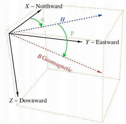
Figure 1: Reference system used to describe the magnetic field ($\mn@boldsymbol{B}$) direction: $\mn@boldsymbol{H}$ is the projection of $\mn@boldsymbol{B}$ onto the horizontal plane. The angles $\hat{q}$ and $\hat{p}$ define the direction with respect to the geographic North (X axis) and the inclination with respect to the local horizontal (orthogonal to Z axis). Downward directions mean positive values.

4 Results

4.1 Frequency templates

Using the procedure and the code described in the previous sections we have been able to evaluate the polarized signal of the atmospheric oxygen for each place on the Earth surface, assuming that the atmospheric parameters (basically pressure and temperature profiles) are available. Earth magnetic field parameters are computed for the year 2010.

We computed the circularly polarized contribution ($V$ Stokes parameter) for the various sites previously mentioned. The absolute value of the signal at the zenith vs frequency is shown in Figure 2. The strong contribution of the single line at 118 GHz and of the ensemble of lines around 60 GHz can be immediately noticed.

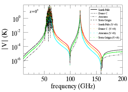
Figure 2: Polarized atmospheric $O_{2}$ signal emitted at the zenith for the various observing sites as a function of the frequency. The absolute value of $V$ is shown. Colored lines denote negative values. Values obtained at Dome C are very similar to those found at Testa Grigia, although the sign is the opposite.

Differences among the various sites are due to a number of reasons. Among them the most important are: 1. the altitude of the observing site since the lower layers of the atmosphere, having an higher pressure (see eq. 12), are the major contributors to the signal; 2. at mid and low latitudes (Atacama and Testa Grigia) the amplitude of the Earth magnetic field is a factor of two weaker than that at South Pole; 3. the amplitude of the effect depends on the scalar product between the line of sight and the Earth magnetic field direction. For sites close to the magnetic poles the magnetic field direction is almost vertical, while at lower latitudes the magnetic field direction is almost horizontal and aligned along the North-South direction.

Black lines in Figure 2 denote values $V>0$ (i.e. right handed circular polarization), while colored lines denote values $V<0$ (i.e. left handed circular polarization). We can notice that the polarized signal at Testa Grigia has a sign reversed respect to other places. This happens because the magnetic field B is directed downward in Testa Grigia (which is in the northern hemisphere), while B is directed upward elsewhere (all the other sites are located in the southern hemisphere). We can notice also a sign reversal at the frequencies $\nu\simeq 99$ GHz and $\nu\simeq 160$ GHz. The first null is originated by the 118 GHz line wing crossing the 50-70 GHz lines wings. The null at higher frequency is originated adding the contribution from lines with $L\geq 9$. Adding lines with higher $L$ the null frequency shifts to lower values, converging to the final value shown in Fig. 2. The coefficients $A_{0}$, $A_{1}$ and $A_{2}$ (see eq. 6 and 7), which assume different values line by line, seem to play an important role in this effect. Anyway, as discussed in section 4.4, it should be stressed that above $\sim$120 GHz the model is not yet validated, and calculation could be not accurate.

4.2 Angular templates

We then built the maps of the polarized signal as seen at the various sites in local alt-azimuthal coordinates. Maps of the polarized signal, at 90 GHz, seen at the selected sites are shown in Figures 3, 4, 5 and 6. Both positive and negative values indicate that both right and left handed circular polarization is present. We find $V=0$ in the maps (red contour) at the angular positions where B is orthogonal to the line of sight. Elevation cuts along the North-South direction and azimuth cuts at constant elevation of 45^∘ of these maps are presented respectively in Figures 7 and 8. Observing in directions different from the zenith the actual signal depends also on the atmospheric thickness. This effect is visible in the elevation scans that show a zenith-secant law dependence. The spatial structure of these maps is dominated by the combination of magnetic field direction and atmospheric thickness in the line of sight. Each map covers a surface, which has a typical scale length of $\sim 200$ km, at an altitude of $\sim 30$ km, corresponding to a multipole $n\sim 200$. The magnetic field components at these multipoles (or even higher) are negligible with respect to the longer wavelength components and not larger than the accuracy of the IGRF-2010 model ($\sim$ 10 nT).

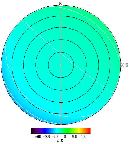
Figure 3: Map of the atmospheric $O_{2}$ circularly polarized signal at Dome C, at frequency $\nu=90$ GHz. The Lambert projection centered at the local zenith, down to 15^∘ of elevation, is shown: upward direction is the geographic North. Black circles denote elevation intervals of 15^∘. Color scale ranges from -750 $\mu K$ to +550 $\mu K$. White contours denote intervals of 50 $\mu K$ in brightness temperature.

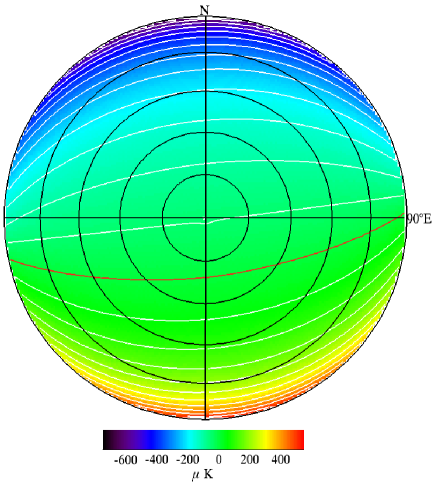
Figure 4: Map of the atmospheric $O_{2}$ circularly polarized signal at Atacama. The red contour denotes the null signal level. See caption of fig. 3 for details.

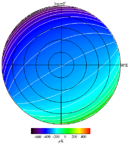
Figure 5: Map of the atmospheric $O_{2}$ circularly polarized signal at South Pole. See caption of fig. 3 for details, but notice that upward direction is the geographic longitude $\ell=0$.

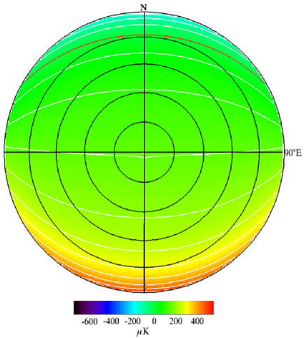
Figure 6: Map of the atmospheric $O_{2}$ circularly polarized signal at Testa Grigia. The red contour denotes the null signal level. See caption of fig. 3 for details.

The effect due to the variation of the atmospheric thickness is combined in the maps with the direction of the magnetic field. At Dome C, where the magnetic field is almost vertical, the two effects compensate each other and the signal is flat on a large part of the visible sky. Conversely at Atacama, where the magnetic field is almost horizontal, the two effects combine increasing the gradient along the visible sky.

The typical signal variation, at 90 GHz, for North-South elevation scans (down to 60^∘ from the zenith) is of the order of 70 $\mu K$ at Dome C, of the order of 300 $\mu K$ at South Pole and Testa Grigia, and of the order of 500 $\mu K$ at Atacama. The typical signal variation for full-360^∘ azimuth scans at $el=45^{\circ}$ is of the order of 50 $\mu K$ at Dome C, of the order of 170 $\mu K$ at South Pole and Testa Grigia, and of the order of 270 $\mu K$ at Atacama.

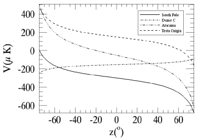
Figure 7: Elevation scans of the Oxygen polarized signal for the several sites. Cuts are taken along the North-South direction. Frequency is $\nu=90$ GHz.

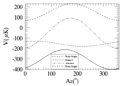
Figure 8: Azimuth scan of the Oxygen polarized signal for the several sites. Cuts are taken at constant elevation (45^∘). Frequency is $\nu=90$ GHz.

The signal gradient has also been computed in order to give a better description of the signal angular dependence. Reference values are summarized in Table 3. The column 3 of Table 3 presents the minimum and maximum gradients in the elevation scans shown in Figure 7, occurring respectively at the zenith and at the lowest elevation. We consider only the central part where $|el|\geq 45^{\circ}$. It can be noticed that the signal variation is minimum ($\sim 0.3-0.8\mu K/^{\circ}$) at Dome C, while the gradient increases by a factor of 4 at South Pole and Testa Grigia and by a factor of 7 at Atacama. The column 4 of Table 3 presents the maximum signal gradient for the azimuth scans of Figure 8. These values indicate that Dome C presents the smoother pattern for the polarized emission from atmospheric $O_{2}$.

Table 3: Typical signals and gradients of the Stokes parameter $V$ at the several sites. Signals are evaluated at 90 GHz. Column 2: total polarized signal at the zenith (see Fig. 2); Column 3: elevation gradient for a North-South scan, minimum (occurring around the zenith) and maximum (occurring al lowest elevation) values for $el\geq 45^{\circ}$ (see Fig. 7); Column 4: maximum azimuth gradient for a scan at $el=45^{\circ}$ (see Fig. 8); Column 5: peak-to-peak polarized signal in a scan at $el=45^{\circ}$ (see Fig. 8); Column 6: azimuth positions where maximum azimuth gradients occur (for azimuth reference see Figs. 3 - 6).

Site	$V_{z}$($\mu K$)	$\frac{\delta V}{\delta\theta_{el}}$($\mu K/^{\circ}$)	$\frac{\delta V}{\delta\phi_{az}}$($\mu K/^{\circ}$)	$\delta V_{pp}(az)$($\mu K$)	$\Phi_{az}$(∘)
Dome C	-153.4	$0.3-0.8$	0.4	50.2	129; 310
South Pole	-299.0	$1.4-3.2$	1.6	188.1	61; 242
Atacama	-52.5	$2.5-5.1$	2.5	288.0	83; 264
Testa Grigia	+147.1	$1.3-2.9$	1.4	158.8	90; 271

By means of our template the $O_{2}$ polarized signal can be computed at any time given the site where the observations are carried out, giving the possibility of subtracting it from the sky signal. For a real experimental setup the signals computed for a given direction have to be integrated with the efficiency of the bandwidth and convolved with the observing beam profile.

4.3 Bands optimization

Astrophysical and cosmological signals can be investigated by ground based experiments through the atmospheric windows, where transparency is large. The opacity of the atmosphere at mm-wave frequency is due to the combined unpolarized emission of (mainly) molecular Oxygen (the same transitions considered for the polarized emission) and water vapor lines (at 22 GHz and 183 GHz). In Fig. 9 the total brightness temperature of the atmosphere at Dome C is shown between 10 GHz and 200 GHz.

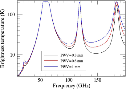
Figure 9: Brightness temperature of the atmosphere at the zenith for Dome C station. The three curves correspond to different values of the precipitable water vapour (PWV=1 mm corresponding to a typical summer condition, PWV=0.6 mm and PWV=0.3 mm corresponding to a typical winter condition).

Inside this interval we define three frequency windows of atmospheric transparency: the first between 25 GHz and 45 GHz, the second between 75 GHz and 110 GHz and the third between 125 GHz and 170 GHz. Inside these frequency intervals it is possible to observe the sky with a transparency larger than 0.8, using a wide bandwidth ($\Delta\nu/\nu=0.2-0.3$). In these frequency bands we estimate the integrated polarized temperature due to atmospheric oxygen. We select 3 ideal rectangular bandpass which are 10 GHz, 20 GHz and 30 GHz wide (i.e. corresponding roughly to a 20% bandpass) respectively for the three bands. The results are shown in Figures 10, 11 and 12 as a function of the central observing frequency.

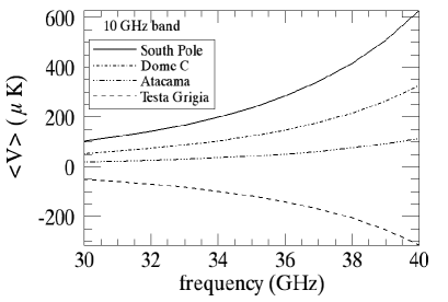
Figure 10: Integrated polarized signal from $O_{2}$ vs the central frequency: bandwidth $\Delta\nu=10$ GHz; frequency interval from 25 to 45 GHz; observing towards the zenith.

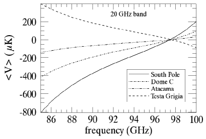
Figure 11: Integrated polarized signal from $O_{2}$ vs the central frequency: bandwidth $\Delta\nu=20$ GHz; frequency interval from 75 to 110 GHz; observing towards the zenith.

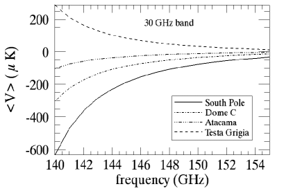
Figure 12: Integrated polarized signal from $O_{2}$ vs the central frequency: bandwidth $\Delta\nu=30$ GHz; frequency interval from 125 to 170 GHz; observing towards the zenith.

This analysis allows us to define the optimal frequency bandwidths for observation of circular polarization inside the windows, while avoiding the largest signals from the peaks and the highest part of the line wings. In the 75-110 GHz interval the high frequency side is preferred because here we find a null in the polarized signal. Therefore the optimal frequency band is 87-107 GHz. Inside the 125-170 GHz interval we do not find a null, but rather a signal that becomes smaller and smaller as we rise the central frequency of our integration band: for this reason, the contamination is smaller in the 140-170 GHz interval. Also in the 25-45 GHz interval there is not a null, therefore the farther from the line tails the smaller the polarized contribution, and the low frequency side is preferred (25-35 GHz). Anyway, it has to be kept in mind that a global optimization of the bandwidth must also consider the unpolarized signal (see Fig. 9) and the true bandwidth transmission.

4.4 Accuracy of the templates

We have estimated the accuracy of the templates at 90 GHz for the various sites, taking into account uncertainties and typical variability of the principal parameters of the model, i.e. the magnetic field and the atmospheric conditions. We first considered the magnetic field⁴ and summarize the results in Table 4, taking into account several sources of uncertainty or variations: 1) We estimated a typical rms uncertainty: $\delta|B|$=20nT, $\delta\hat{p}$=$\delta\hat{q}$=1^′. But at Dome C and South Pole we consider $\delta\hat{q}$=5^′. This uncertainty includes both the quoted error bars of the IGRF model and the unaccounted contribution of the spatial frequencies higher than $n=13$. Results, obtained using a Monte Carlo for these parameters, are reported in column 3 of Table 4. 2) Then we evaluated the secular variation (SV) of the magnetic field, for the various sites. We considered the consolidated values for the past since 2005 and the forecast values for the next years up to 2015. We found a nearly linear variation with time, which we reported in column 4 of Table 4. Using the magnetic field values obtained for the several years we computed the amplitude of the atmospheric circular polarization. We found again a nearly linear variation with time, reported in column 5 of Table 4. At Atacama the change of magnetic field direction plays an important role, in particular at the zenith, while in all the other sites the strength variation is dominating. 3) Finally we evaluated the variation of the atmospheric circular polarization in case of an intense magnetic storm when the magnetic field strength changes as much as $\sim$ 1000 nT. Usually magnetic disturbances last no more than a few days and afterwords quiet conditions are established again. Results, which represent unusual maximum short-time variations, are reported in column 6 of Table 4.

Table 4: Typical polarized signal uncertainties or variations due to the amplitude od the Earth magnetic field. We evaluated the effect at the zenith and at ($el$=$45^{\circ}$ ; $az$=0). Column 3: rms error bar due to the IGRF model uncertainties. Column 4: Secular variation of the magnetic field. Column 5: change of the signal due to SV of magnetic field. Column 6: signal variation due to a typical big magnetic disturbance (md).

Site	Elevation	$\delta V_{rms}$($\mu K$)	$\frac{\delta|B|_{sv}}{\delta t}$($nT/y$)	$\frac{\delta V_{sv}}{\delta t}$($\mu K/y$)	$\delta V_{md}$($\mu K$)
Dome C	90∘	$0.05$	-21	$+0.05$	$\sim$ 3
Dome C	45∘	$0.07$	-21	$+0.13$	$\sim$ 2
South Pole	90∘	$0.11$	-63	$+0.38$	$\sim$ 5
South Pole	45∘	$0.16$	-63	$+0.44$	$\sim$ 7
Atacama	90∘	$0.06$	-52	$-0.27$	$\sim$ 2
Atacama	45∘	$0.17$	-52	$+0.23$	$\sim$ 9
Testa Grigia	90∘	$0.07$	+26	$+0.12$	$\sim$ 3
Testa Grigia	45∘	$0.07$	+26	$+0.04$	$\sim$ 1

We then considered the atmospheric parameters and summarize the results in Table 5. We limited our analysis to Atacama¹ Dome C and South Pole² because of the poor statistics available for Testa Grigia. We took into account several sources of uncertainty or variations: 1) We estimated the uncertainty due to the accuracy of the measurements in the temperature and pressure profile. We took the values quoted by Tomasi et al. (2006) ($\delta P_{exp}=5$ mb, $\delta T_{exp}=0.5$ K). Results ($\delta V_{exp}$), obtained using a Monte Carlo distribution for these parameters, are reported in column 3 of Table 5. 2) We then estimated the variability of $T$ and $P$ comparing several measured profiles, taken in different days, but equivalent conditions. We found a nearly equivalent rms variation for the various sites: $\delta P_{st}\simeq 0.8$ mb, $\delta T_{st}\simeq 2.0$ K. Using these variabilities we obtain $\delta V_{st}$, the signal variation reported in column 4 of Table 5. We searched also for a day-night variation, but we found that it is limited to the temperature of the lowest layers of the atmosphere. The effect we found is not larger than $\delta V_{st}$. 3) We also estimated the seasonal long-term variability of the atmospheric parameters. We compared measured profiles taken several months later and evaluated the maximum variation of $T$ and $P$. We found that at Atacama the variation, even if relevant, is still limited to the lowest layers of the atmosphere. Conversely at Dome C and South Pole the seasonal variation impacts the full air column. In columns 5 and 6 of Table 5 we report the typical maximum seasonal variation measured in the lowest layers of the atmosphere (the maximum temperature variation at the ground is usually even larger). Results on the polarized signal ($\delta V_{lt}$) are reported in column 7 of Table 5.

Table 5: Typical polarized signal uncertainties or variations due to the atmospheric parameters. We evaluated the effect at the zenith and at ($el$=$45^{\circ}$ ; $az$=0). Column 3: rms error bar due to temperature and pressure profile measurement uncertainties ($\delta P=5$ mb, $\delta T=0.5$ K). Column 4: signal variation due to short-term rms variation of temperature and pressure. Column 5: typical seasonal (long-term) temperature variation. Column 6: typical seasonal (long-term) pressure variation. Column 7: signal variation due to a typical seasonal (long-term) variation.

Site	Elevation	$\delta V_{exp}(\mu K)$	$\delta V_{st}(\mu K)$	$\delta T_{lt}(K)$	$\delta P_{lt}(mb)$	$\delta V_{lt}(\mu K)$
Dome C	90∘	0.7	0.5	36	15	3.4
Dome C	45∘	0.7	0.5	36	15	2.9
South Pole	90∘	1.1	0.8	26	15	10.0
South Pole	45∘	1.4	1.1	26	15	13.7
Atacama	90∘	0.1	0.1	10.5	2.6	0.23
Atacama	45∘	0.6	0.3	10.5	2.6	0.9

As shown by Tables 4 and 5 the accuracy is of the order of $\mu$K. Larger effects arise in case of large magnetic disturbances or seasonal changes. We did not take into account the line profile model. The line frequencies are known with negligible error bars, but the Oxigen absorption values have error bars of at least 5% at 90 GHz. This accuracy applies up to $\sim$ 120 GHz, but at higher frequencies model and values of Oxigen absorption are not yet validated and calculations should be used with caution. The effect of these uncertainties should be added to the accuracy quoted previously. It is also important to stress that the computed uncertainty refers to the total power polarized signal. Usually we are interested to subtract signal gradients between different observing directions, and the related uncertainty is definitely smaller than the total estimated value of $\delta V$, in particular for small angular scales.

5 Conclusions

In this paper we evaluate the contribution of atmospheric $O_{2}$ Zeeman split roto-vibrational lines in the mm-wave part of the electromagnetic spectrum, seen as a contaminant for CMB polarization experiments. A code to simulate this signal for various sites (Dome C and South Pole in the Antarctica, Testa Grigia in the Italian Alps and Atacama, Chile) of interest for mm-wave astronomy has been developed on the basis of the theory developed in Lenoir (1967) and Lenoir (1968)). In this way we compute a template of the atmospheric circularly polarized signal for every site provided that the vertical profiles of atmospheric pressure and temperature are available.

Maps of the circularly polarized signal in local coordinates have been obtained for each site examined. These maps show a dipole-like large scale feature with a maximum gradient aligned approximately, for low-mid latitude sites, with the North-South direction, and for polar sites, along the magnetic field lines. Atacama is the examined place where the polarized signal at the zenith is the lowest. This is due to the altitude of the site and to the amplitude and direction of the magnetic field. Unfortunately scanning experiments at Atacama suffer a larger polarized gradient with respect to other sites. In fact the angular variation of the signal is of order $\sim 1.3-5.1\ \mu K/^{\circ}$ at 90 GHz for all sites except Dome C, where it is a factor $\sim$ 4$-$7 lower, because here the atmospheric polarized signal is the flattest, along the full local visible sky.

We then evaluated the integrated polarized signal inside an ideal bandpass of a wide-band ($\Delta\nu/\nu=0.2$) experiment for 3 mm-wave atmospheric windows between 10 and 200 GHz. We found the frequencies where it is more convenient to observe, because here the signal vanishes or decreases significantly. Finally, an estimate of the template accuracy and variation has been done, using the main features of the magnetic field and the statistics of measured atmospheric profiles. At 90 GHz, we obtained a typical uncertainty of the order of $\sim$ 1 $\mu$K, dominated by accuracy and variability of the atmospheric parameters. Large variations (up to $\sim$ 10-15 $\mu$K) are expected in case of large magnetic disturbances and due to seasonal atmospheric variations. Uncertainty and secular variation of the magnetic field have, on the other hand, a negligible effect.

A linear polarization is also generated and it is larger when the line of sight is orthogonal to the Earth magnetic field. However the ratio of linear to circular polarization is $\sim 10^{-4}$, therefore still below the current detection sensitivity. Moreover the non vanishing component of linear polarization is nearly aligned with the Earth magnetic field.

Acnowledgments

Authors want to acknowledge P. Rosenkranz and S. Hanany for the precious contribution to the improvement of the paper. Data from Dome C are Copyright of Italian PNRA (http:$//$www.climantartide.it).

References

- Agarwal et al. (2008) Agarwal N., et al., 2008, PRD, 78, 085028-1/11.
- Alexander et al. (2009) Alexander S., Ochoa J., Kosowsky A., 2009, PRD, 79, 063524-1/17.
- Carlson & Garretson (1994) Carlson E.D., Garretson W.D., 1994, Phys. Lett. B, 336, 431-438.
- Carroll & Field (1991) Carroll S. M., Field G. B., 1991, PRD, 43, 12, 3789-3793.
- Cooray et al. (2003) Cooray A., Melchiorri A., Silk J., 2003, Phys. Lett. B, 554, 1-6.
- De Petris (2008) De Petris M., 2008, private communication.
- Finelli & Galaverni (2009) Finelli F., Galaverni M., 2009, PRD, 79, 063002-1/15.
- Giovannini (2009) Giovannini M., 2009, PRD, 80, 123013(6).
- Giovannini (2010) Giovannini M., 2010, PRD, 81, 023003(24).
- Hanany & Rosenkranz (2003) Hanany S., Rosenkranz P., 2003, New Astr. Rev., 47 n.11, 1159.
- Harari & Sikivie (1992) Harari D., Sikivie P., 1992, Phys. Lett. B, 289, 67-72.
- Hu & White (1997) Hu W., White M., 1997, New Astronomy, 2, no. 4, 323-344.
- Hulot et al. (2002) Hulot G., Eymin C., Langlais B., Mandea M., Olsen N., 2002, Nature, 416, 620-623.
- Keating et al. (1998) Keating B., Timbie P., Polnarev A., Steinberger J., 1998, ApJ, 495, 580-596.
- Lenoir (1967) Lenoir W. B, 1967, JAP,38, 5283-5290.
- Lenoir (1968) Lenoir W. B, 1968, J. Geophys. Res., 73, 361.
- Liebe et al. (1992) Liebe H. J., Rosenkranz P. W., Hufford G. A., 1992, J. Quant. Spectrosc. Radiat. Transfer, 48, 629-643.
- Lubin et al. (1983) Lubin P., Melese P., Smoot G., 1983, ApJ 273, L51-L54.
- Partridge et al. (1988) Partridge R. B., Nowakowski J., Martin H. M., 1988, Nature, 331, 146-147.
- Pietranera et al. (2007) Pietranera L., Buehler S.A., Calisse P.G., Emde C., Hayton D., John V.O., Maffei B., Piccirillo L., Pisano G., Savini G., and Sreerekha T.R., 2007, MNRAS, 376, 645-650.
- Rosenkranz & Staelin (1988) Rosenkranz P. W., Staelin D. H., 1988, Radio Sci., 23, 721-729.
- Tomasi et al. (2006) Tomasi C., et al., 2006, J. Geophys. Res., 111, D20305.
- Van Vleck & Weisskopf (1945) Van Vleck J. H., Weisskopf V. F., 1945, Rev. Mod. Phys., 17, 227-236.