Spectral stability of vortices in two-dimensional
Bose-Einstein condensates via the Evans function
and Krein signature

Abstract

We investigate spectral stability of vortex solutions of the Gross-Pitaevskii equation, a mean-field approximation for Bose-Einstein condensates (BEC) in an effectively two-dimensional axisymmetric harmonic trap. We study eigenvalues of the linearization both rigorously and through computation of the Evans function, a sensitive and robust technique whose use we justify mathematically. The absence of unstable eigenvalues is justified a posteriori through use of the Krein signature of purely imaginary eigenvalues, which also can be used to significantly reduce computational effort. In particular, we prove general basic continuation results on Krein signature for finite systems of eigenvalues in infinite-dimensional problems.

1 Introduction

Background. Since the experimental creation of Bose-Einstein Condensates (BEC) in alkali vapors in 1995 [5, 13], BEC are one of the most active areas of modern condensed-matter physics. A general overview of the subject can be found in [12, 58], and particularly in the review book [42]. In the Hartree-Fock mean-field approximation, BEC are modeled by the nonlinear Schrödinger equation (NLS) with a non-local nonlinearity. A traditional simplification, replacing the non-local interaction potential with a localized short-range interaction proportional to the delta function, leads to the Gross-Pitaevskii equation

$$i\hbar\psi_{t}=\left(-\frac{\hbar^{2}}{2M}{\mathbf{\triangle}}+V({\bf x})+i\hbar\Omega\partial_{\theta}+g|\psi|^{2}\right)\psi\,,$$ (1)

where $\hbar$ is Planck’s constant, $M$ is the atomic mass of atoms in the condensate, $\theta$ is an azimuthal angle in cylindrical coordinates, and $g$ is an interaction strength parameter. The total number of particles $N$ in the condensate is given by the integral

$$N=\int_{\mathbb{R}^{3}}|\psi|^{2}dx^{3}\,,$$ (2)

and is conserved during the evolution of the system. Equation (1) is a nonlinear Schrödinger equation with a cubic nonlinearity (focusing or defocusing depending on whether the interaction is attractive or repulsive, respectively) and with a spatially dependent trap potential $V({\bf x})$ stationary in a frame rotating with frequency $\Omega$ about the vertical axis. A rigorous mathematical justification of the Gross-Pitaevskii model for the BEC ground state under various conditions directly from many-body Schrödinger equations was done in a series of papers of Lieb et al. [45]–[49].

From the point of view of nonlinear waves, the interesting phenomena is that the Gross-Pitaevskii equation, similarly to some other nonlinear Schrödinger equations, supports the existence of various types of solitary wave solutions. In the two-dimensional setting we will study in particular, there are vortex solutions which have the form

$$\psi(t,r,\theta)=e^{-i\mu t}e^{im\theta}w(r),$$

where $r,\theta$ are polar coordinates, $m$ is vortex degree, $\mu$ is the vortex rotation frequency (physically, chemical potential) and $w(r)$ is the radial vortex profile.

Problems of stability for vortex solutions to various forms of nonlinear Schrödinger equations have drawn much attention in recent years. Related questions for models arising from nonlinear optics, micromagnetics and Bose-Einstein condensation have been considered extensively in the mathematical and physical literature. For recent work concerning spectral stability questions for various types of matter-waves, including vortices, vortex rings, multi-poles, soliton and vortex necklaces in the presence of magnetic traps and optical lattices, see for example [36, 37, 38, 42, 43]. Rigorous mathematical results on these questions are rather few, however, due to the strong nonlinearity and complexity of the system.

This work. In the present work we study the spectral stability of a single two-dimensional axisymmetric vortex trapped in an axisymmetric harmonic trap. For this simple well-studied physical setting, we develop an approach that involves a combination of analytical and numerical tools which allows us to obtain reliable results for large particle number, well into the Thomas-Fermi regime (e.g. $N\sim 10^{6}$ atoms of   ²³${}_{\rule{0.0pt}{5.25pt}}$Na). It is important to note that in the present axisymmetric setting, rotation of the trap does not influence the dynamic stability of vortices, as the rotation term can be removed by transforming to an appropriately rotating coordinate frame.

Analytical results. Our study involves a number of analytical results that we prove in sections 5 and 6 concerning the spectrum of the operator one obtains by linearizing about a vortex solution. In section 5, we prove that due to the harmonic trapping potential the essential spectrum of this operator is empty — hence the spectrum consists entirely of isolated eigenvalues of finite multiplicity. The real part of any eigenvalue satisfies an explicit bound depending only on the (non-dimensionalized) frequence $\mu$ and degree $m$ of the vortex, namely

$$|\mathop{\rm Re}\nolimits\lambda|<3(\mu-m)\,.$$ (3)

The eigenvalue problem breaks into an infinite system of coupled pairs of ordinary differential equations (ODEs) for azimuthal Fourier modes indexed by $j\in\mathbb{Z}$. As is known from [18], only finitely many of these are relevant for possible instability, namely the ones satisfying

$$0<|j|<2m.$$ (4)

We construct a globally analytic Evans function [3, 15] associated with each of the ODE pairs, whose zeros correspond to the eigenvalues. These results extend the approach of [54] for focusing-defocusing nonlinear Schrödinger equations to handle a harmonic trapping potential.

One of the weaknesses in the numerical investigations in [54] was that one could not be confident that all unstable eigenvalues were detected, due to the absence of any bound on their imaginary part. No such bound is available in the present problem either. Nevertheless, we will show how one can indeed account for all possible instabilities through use of Krein signature (the sign of the linearized energy of associated eigenmodes).

The key property of Krein signature that makes it useful is its invariance under continuous variation of parameters such as the standing-wave frequency $\mu$ and the size of the condensate. In section 6 we extend results that are well-known for finite-dimensional systems to establish a general continuation property for any family of operators that is resolvent-continuous, a natural notion of weak continuity that one expects to hold in many applications to infinite-dimensional systems. Preservation of a definite signature is proved for any finite system of imaginary eigenvalues for such a family. By consequence, the only way eigenvalues can leave the imaginary axis is through collision with eigenvalues of opposite Krein signature.

There are three reasons why Krein signature is extremely helpful and a powerful tool in the present work. First, it allows us to explain the collisions (or avoided collisions) of eigenvalues found in our numerical computations. Moreover, in combination with numerical plots, it provides a numerically convincing a posteriori justification that there are no unstable eigenvalues outside a certain fixed box in the complex plane. Finally, it can be used to significantly reduce the amount of necessary computation, as we shall discuss in section 7.2.

Numerical methods. In order to locate zeros of the Evans functions using the argument principle, we design and implement a numerical method somewhat more robust than that used in [54]. We use a path-following technique and multiple shooting to compute the nonlinear wave profile, and a rescaled exterior-product representation of the Evans function to handle problems of rapid growth and numerical dependence. A numerical path-following technique for radially symmetric profiles was also used by Edwards et al. [14].

Numerical results. In agreement with previous studies in the physical literature [18, 37, 60, 68], we find a singly-quantized vortex $(m=1)$ spectrally stable while the stability of multiply-quantized vortices (with $m=2$ and 3) depends on the diluteness of the condensate, with alternating intervals of stability and instability as $Ng$ varies. Pu et al. [60] in their analysis use a different numerical method (finite elements) which is a priori less reliable and sensitive than the approach used here. Moreover, our results account for the appearance of all instabilities through the tracking of all eigenvalues of negative Krein signature. The presence of unstable eigenvalues (eigenvalues with positive real part) for certain parameters is also corroborated by direct simulation of time-dependent dynamics based on the splitting scheme proposed in [6].

Symmetries. In the computations one observes a special set of eigenvalues which remain constant under variation of standing-wave frequency and condensate size. These eigenvalues arise from the symmetries of the Gross-Pitaevskii equation, as we discuss in an appendix. One symmetry is particularly interesting — a breather boost, which we found first described in [59]. This is self-transformation of the Gross-Pitaevskii equation related to the Talanov lens transformation, involving a time-periodic dilation of space with an appropriate radial phase adjustment. This symmetry corresponds to eigenvalues $\pm 2{\rm i}\omega$ of the Gross-Pitaevskii equation with the harmonic potential $V({\bf x})=\frac{1}{2}{\omega^{2}}|{\bf x}|^{2}$, linearized about a central vortex, with mode shapes corresponding to infinitesimal breathing oscillations.

Related literature. Let us now discuss some known results on stability which are relevant to our problem. In general, two different concepts of stability are distinguished in the literature: energetic and dynamic stability. A solution is energetically stable if it minimizes an associated energy functional within a certain class of functions.

The simplest energetic stability approach, where the minimization takes into account only single vortex solutions with different charges, indicates that a high enough trap rotation frequency can eventually stabilize a vortex of any degree [8]. On the other hand, without external trap rotation, the energy of a single multi-quantized vortex of charge $m$ is larger than the energy of $m$ singly-quantized vortices, and thus multi-quantum vortices are believed to be unstable. The total energy in this case also depends on the relative location of vortices as they tend to form regular hexagonal arrays in harmonic traps.

A mathematical framework for a rigorous variational approach was discussed by Aftalion and Du [2]. Their method for effectively 2D condensates is parallel to the Ginzburg-Landau theory of superconductors. In [66] the authors claim that sufficiently fast rotation in combination with a strong pinning potential is capable of making even multi-quantum vortices energetically stable.

A detailed rigorous analysis was conducted by Seiringer [65], who studied regimes when a vortex solution can be a global energy minimizer. He proves that for any $0<\Omega<\Omega_{c}$ there exists $m_{\Omega}$ (independent of an interaction potential) such that all vortices with charge $m>m_{\Omega}$ are energetically unstable; i.e., they are not global minimizers (ground states) of the energy functional (see also [30]). Moreover, he proves that all multi-quantized vortices, $m\geq 2$, become energetically unstable for a large enough value of the chemical potential of the condensate. Finally, he proves that symmetry breaking of the axisymmetric vortex solution is inevitable for any $m$, even for a singly-quantized vortex for a large enough interaction strength, since no ground state is an eigenfunction of the angular momentum. The symmetry breaking of a one-dimensional ground state is also demonstrated by a dynamical systems analysis in [33] in the case of a double-well trapping potential.

Energetic stability provides a sufficient condition for dynamic stability — ground states of the energy functional are nonlinearly orbitally Lyapunov stable, i.e., if the initial data are “close” to the ground state solution then the perturbed solution remains “close” to the ground state solution for all times. (See [33] for a detailed dynamic stability study of a one-dimensional model and a sketch of the proof of well-posedness for the initial-value problem for the Gross-Pitaevskii equation.) As dynamic stability need not imply energetic stability, however, it may not be possible to draw conclusions on dynamic instability directly from considerations of the energy functional. The study of linear or spectral stability can be helpful since one may detect possible instabilities due to the presence of eigenvalues in the right half-plane.

In the physical literature, García-Ripoll and Pérez-García [18] and Pu et al. [60] have studied linear stability of single multi-quantized vortices using equations equivalent to those here. The numerical results of [60] agree substantially with those of the present paper. In [18] the search for instability is restricted only to the so-called anomalous modes – modes with a negative linearized energy. As pointed out in [31] for example, these modes are not intrinsically unstable in the sense that some dissipation mechanism must be introduced into the system for them to become relevant. The numerical techniques used in [18] and [60] rely on Galerkin-type approximations. A finite-temperature generalization is further studied in [71].

Use of the Krein signature as a tool to study stability of nonlinear waves has appeared recently in various studies, see [9, 26, 34, 39, 56] and references therein. Skryabin in [67] (also see [68]) studies a binary mixture of trapped condensates using such information. Kapitula et al. [37] study stability of various types of matter-waves including localized vortices. Their perturbation argument, combined with topological methods based on Krein signature, describes in detail transition to instability in the limit of weak atomic interactions. Finally, Kapitula and Kevrekidis [35, 36] have studied Bose-Einstein condensates in the presence of a magnetic trap and optical lattice, making efficient use of information on the Krein signature of relevant eigenvalues.

Organization of this paper. First, Sections 2 and 3 introduce notation and recall background results regarding the Gross-Pitaevskii equation and vortex solutions. Section 4 contains most of our analytical results, concerning linearization, essential spectrum, bounds on eigenvalues, and reduction to ODEs. Moreover, we establish a precise asymptotic description of eigenfunctions necessary for construction of the Evans function. The Evans function itself is constructed in Section 5. In Section 6, we discuss the Krein signature. We describe in detail our numerical procedure and discuss the numerical results in Section 7. Finally, in an Appendix we discuss symmetries and boosts of the problem and relate them to the eigenvalues which do not change as the standing wave frequency varies.

2 The Gross-Pitaevskii Equation

The behavior of low-temperature Bose-Einstein condensates (BEC) trapped in the harmonic potential $V({\bf x})$ rotating with the angular velocity $\Omega$ about the $z$-axis is well described by the time-dependent Gross-Pitaevskii equation. The wave function $\psi({\bf x},t)$ satisfies (1) (in three dimensions) with trapping potential $V({\bf x})=V(x,y,z)$ given by

$$V({\bf x})=V_{3D}({\bf x})=\frac{1}{2}M\left(\omega_{x}^{2}x^{2}+\omega_{y}^{2}y^{2}+\omega_{z}^{2}z^{2}\right)\,.$$

The interaction strength parameter $g$ is

$$g=g_{3D}=\frac{4\pi\hbar^{2}a}{M}\,,$$

where $a$ is the $s$-wave scattering length [45]. The term $\Omega\partial_{\theta}$ corresponds to the angular momentum ${\mathbf{\Omega}}\cdot({\mathbf{r}}\times{\mathbf{\nabla}})$ of the condensate caused by a rotating frame of coordinates. The total number of particles in the condensate $N$ is given by the integral

$$\int_{\mathbb{R}^{3}}|\psi|^{2}dx^{3}=N\,,$$ (5)

and is conserved during the evolution of the system. For disc-shaped (pancake) traps ($\omega_{z}^{2}\gg\omega_{x}^{2}$, $\omega_{z}^{2}\gg\omega_{y}^{2}$) it was justified [6] that the system is well approximated by a planar two-dimensional reduced model. The equation (1) formally does not change; one only needs to set

$$V(x) = V_{2D}(x)=\frac{1}{2}M\omega_{tr}^{2}\left(x^{2}+\lambda_{tr}^{2}y^{2}\right)\,,$$

$$g = g_{2D}=g_{3D}\cdot\left(\frac{M\omega_{z}}{2\pi\hbar}\right)^{1/2}\,,$$

where $\omega_{x}=\omega_{tr}$ and $\omega_{y}=\omega_{tr}\lambda_{tr}$. For purpose of numerical investigations in this work the same values of parameters were used as in [60]: a condensate consisting of atoms of   ²³${}_{\rule{0.0pt}{5.25pt}}$Na is considered with $a=2.75$ nm, $\omega_{z}=2\pi\times 200$ Hz, $\omega_{tr}=2\pi\times 10$ Hz ($\omega_{z}\gg\omega_{tr}$), $M=10^{-26}$ kg and the Planck constant $\hbar=6.6261\times 10^{-34}$ Js. A similar set of parameters used in the experiment as cited in [32, 66] with a   ⁸⁷${}_{\rule{0.0pt}{5.25pt}}$Rb condensate is: $M=3.81\times 10^{-26}$ kg, $a=5.77$ nm, $\omega=\omega_{z}=\omega_{tr}=2\pi\times 200$ Hz. In these experiments the number of particles was approximately $N=2\times 10^{5}$, horizontal and vertical condensate sizes were $R=20$ $\mu$m, $L=10$ $\mu$m and the temperature $T_{c}=1$ $\mu$K. Both   ²³${}_{\rule{0.0pt}{5.25pt}}$Na and   ⁸⁷${}_{\rule{0.0pt}{5.25pt}}$Rb represent alkali gases with a repulsive interaction potential. As an example of an attractive interaction,  ⁷${}_{\rule{0.0pt}{5.25pt}}$Li with $a=-1.45$ nm can serve. Note that the parameter $a$ can be tuned via Feshbach resonance.

In this work the following assumptions will be made. We assume that the magnetic trap is axisymmetric ($\lambda_{tr}=1$). Thus only two-dimensional wave functions of the form $\psi=\psi(t,r,\theta)$ will be considered. The symmetry of the trap also eliminates dependence of stability of axisymmetric vortices on the trap rotation. Hence, we will set ${\Omega}=0$. Moreover, although the model includes both attractive and repulsive interaction interparticle potential (sign of the nonlinear term), for simplicity only the more interesting case of repulsive potential will be considered here (some results concerning stability in transition between repulsive and attractive potential can be found in [60]).

To nondimensionalize the equation (1) we use the following scaling

$$t=(1/\omega_{tr})\,t^{\prime}\,,\qquad x=\sqrt{{\hbar}/{M\omega_{tr}}}\,x^{\prime}\,,\quad\psi=\sqrt{\hbar\omega_{tr}/{|g|}}\,\psi^{\prime}\,.$$

The Gross-Pitaevskii equation is then expressed (dropping the primes) as

$$i\psi_{t}=-\frac{1}{2}{\mathbf{\triangle}}\psi+\frac{1}{2}r^{2}\psi+|\psi|^{2}\psi$$ (6)

with

$$\int_{0}^{\infty}\int_{0}^{2\pi}|\psi|^{2}r\,d\theta\,dr=K=|g|NM/\hbar^{2}\,.$$ (7)

The energy functional is given by

$$E(\psi)=\int_{0}^{\infty}\int_{0}^{2\pi}\left[\frac{1}{2}|{\mathbf{\nabla}}\psi|^{2}+\left(\frac{1}{2}r^{2}+|\psi|^{2}\right)|\psi|^{2}\right]\,rd\theta\,dr\,.$$ (8)

Note that the Thomas-Fermi regime [16, 45] $Na/d_{0}>>1$ (here $d_{0}$ is the mean oscillator length, $d_{0}=\sqrt{\hbar/M\omega_{0}}$ and $\omega_{0}$ is the mean trap frequency $\omega_{0}^{3}=\omega_{x}\omega_{y}\omega_{z}$) corresponds to $K\rightarrow\infty$ since $K=2|a|N\sqrt{2\pi M\omega_{z}/\hbar}$, i.e.,

$$K=\frac{N|a|}{d_{0}}2\sqrt{2\pi}\left(\frac{\omega_{tr}}{\omega_{z}}\right)^{1/3}\,.$$ (9)

This is the limit under which Lieb and Seiringer [45] justified the Gross-Pitaevskii energy functional to be a good approximation for the $N$-body quantum system. Note, that the only free parameter which stays in (6)–(7) is $K$, the $L^{2}$-norm of the wave function $\psi$.

3 Vortex Solutions

In this section we describe the structure of vortex solutions [51] to the Gross-Pitaevskii equation (6), of the form

$$\psi(t,r,\theta)=e^{-i\mu t}e^{im\theta}w(r),$$ (10)

and describe the numerical procedure which allows us to approximate them with high precision. Here $m$ is an integer, and in this paper it suffices to always assume that $m\geq 1$ due to reflection symmetry.

The radial profile function $w(r)$ of a vortex solution satisfies the equation

$$-w_{rr}-\frac{1}{r}w_{r}+\frac{m^{2}}{r^{2}}w+r^{2}w+2|w|^{2}w-2\mu w=0\,,\quad r>0.$$ (11)

We will require that the radial profiles be non-negative and spatially localized, i.e., satisfy the boundary conditions

$$w(r)\ \mbox{is bounded as $r\rightarrow 0^{+}$,}\quad w(r)\rightarrow 0^{+}\ \mbox{as $r\rightarrow\infty$.}$$ (12)

We note that the boundary condition as $r\rightarrow 0^{+}$ implies $w(r)\rightarrow 0^{+}$ for $m\geq 1$.

Existence. The existence of positive solutions to (11) for some $\mu$, corresponding to any given $K>0$ in (7), can be proved using a well-known variational argument [65]. One minimizes (8) among functions with the spatial dependence in (10), with $m$ and $K$ fixed, and a minimizer may be found that is positive. For any positive solution of (11) with finite energy, necessarily $\mu>m+1$, since multiplying (11) by $2\pi rw$ and integrating in $r$ yields

$$\mu K>\pi\int_{0}^{\infty}\left(w_{r}^{2}+\left(\frac{m^{2}}{r^{2}}+r^{2}\right)w^{2}\right)r\,dr\geq(m+1)K.$$ (13)

The last inequality follows since the integral is minimized at a positive solution of

$$-w_{rr}-\frac{1}{r}w_{r}+\frac{m^{2}}{r^{2}}w+r^{2}w-2\hat{\mu}w=0\,,$$ (14)

which is (11) linearized at zero. Analysis of this equation (see below) yields $\hat{\mu}=m+1$, $w=cw^{(m)}_{0}$ from (18) below, where $c$ is constant.

The following proposition describes a global bound on any vortex solution with positive profile. A proof can be found in [44] (except for the statement that $\mu>m+1$). The bound (13) was also proved in [65].

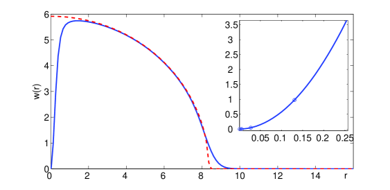
Figure 1: The radial vortex profile of a multi-quantized vortex, $m=2$, for the dimensionless parameter $\mu\approx 35$ corresponding to $N\approx 10^{6}$ particles of   ²³${}_{\rule{0.0pt}{5.25pt}}$Na. The quadratic profile in the Thomas-Fermi regime for the same parameters is also plotted (dashed line). Detailed (quadratic) behavior close to the origin is on the inset.

Proposition 1.

Let $w(r)$ be a finite-energy positive solution to (11), satisfying (12), where $m>0$ is an integer. Then $\mu>m+1$, and $w(r)$ is increasing on $(0,R)$ and decreasing on $(R,\infty)$, for some $R\in(m/\sqrt{2\mu},\sqrt{2\mu})$. Moreover, for all $r>0$ we have

$$|w(r)|^{2}<\mu-m.$$ (15)

The asymptotic behavior of a vortex profile can be determined directly from (11) (see Fig. 1). It is not difficult to see that as $r\rightarrow 0^{+}$ the equation has the same character as the linear Schrödinger equation (14) (one argues as in [29]), and

$$w(r)\sim d_{0}r^{m}\quad\mbox{for $m\geq 1$,}$$

for some positive constant $d_{0}$. As $r\rightarrow\infty$, the nonlinear term for a localized solution becomes negligible and the linear equation (14) is again a good approximation. The proof that the positive solution $w(r)$ to (11) approaching 0 as $r\rightarrow\infty$ satisfies

$$w(r)=O(r^{\mu-1}e^{-r^{2}/2})$$

is also given in detail in [44].

The goal of this paper is to study spectral stability of solutions to (11) both analytically and numerically. Naturally, for a careful numerical stability investigation it is crucial to obtain very precise numerical solutions of (11) first. The approach used here is based on path-following along a branch bifurcating out of the trivial solution $w=0$ and is similar to the one used in [14].

Bifurcation. The bifurcation (and later stability) analysis requires detailed information about the localized solutions to (14). This equation has two independent general solutions — products of a polynomial, a decaying Gaussian and a confluent hypergeometric function. The exact solutions (taking $\hat{\mu}=\mu$ henceforth) are

$$w_{(1)}(r) = r^{m}e^{-r^{2}/2}M\left(\frac{m+1-\mu}{2},m+1,r^{2}\right)\,,$$

$$w_{(2)}(r) = r^{m}e^{-r^{2}/2}U\left(\frac{m+1-\mu}{2},m+1,r^{2}\right)\,.$$

The confluent hypergeometric functions $M(a,b,x)$ and $U(a,b,x)$ are, in general, independent solutions to $xf^{\prime\prime}+(b-x)f^{\prime}-af=0$ [1]. Their asymptotics as $r\rightarrow 0^{+}$ and as $r\rightarrow\infty$ is, respectively,

$$w_{(1)}(r) \sim r^{m}\left(1+O(r^{2})\right)\,,\qquad w_{(1)}(r)\sim\displaystyle\frac{\Gamma(m+1)}{\Gamma(\frac{m+1-\mu}{2})}r^{-\mu-1}e^{r^{2}/2}\left(1+O(1/r^{2})\right),$$

$$w_{(2)}(r) \sim \displaystyle\frac{\Gamma(m)}{\Gamma(\frac{m+1-\mu}{2})}r^{-m}\left(1+O(r^{2})\right)\,,\quad w_{(2)}(r)\sim r^{\mu-1}e^{-r^{2}/2}\left(1+O(1/r^{2})\right).$$

The Wronskian of $w_{(1)}(r)$ and $w_{(2)}(r)$ is given by

$$W(w_{(1)},w_{(2)})=-\frac{2}{r}\frac{\Gamma(m+1)}{\Gamma(\frac{m+1-\mu}{2})}\,.$$ (16)

The only possibility for $w_{(1)}(r)$ (and similarly for $w_{(2)}(r)$) to satisfy the boundary conditions at both ends is when the Wronskian (16) vanishes. This happens if $|\Gamma((m+1-\mu)/2)|=\infty$, so $m+1-\mu=-2n$, $n$ a nonnegative integer. Therefore a non-trivial solution $w_{n}(r)$ to (14) approaching zero as $r\rightarrow 0^{+}$ and as $r\rightarrow\infty$ exists if and only if $\hat{\mu}=\mu_{n}$, where

$$\mu_{n}=m+1+2n,\quad n=0,1,2,\ldots\,.$$ (17)

For $\mu$ given by (17) both solutions $w_{(1)}(r)$ and $w_{(2)}(r)$ reduce to a constant multiple of the single solution

$$w_{n}^{(m)}(r)=r^{m}e^{-r^{2}/2}L_{n}^{(m)}(r^{2}),$$ (18)

where $L_{n}^{(m)}(r)$ is the generalized Laguerre polynomial, with $n$ the number of zeros of $L_{n}^{(m)}(r)$ for $r>0$. The positive solution (the ground state of the associated energy functional) corresponds to $n=0$, $\mu_{0}=m+1$ and $w=w_{0}^{(m)}$.

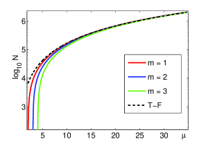
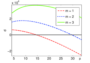
Figure 2: Left panel: ($\log_{10}N$ vs. $\mu$) plot of branches of vortex solutions for $m=1,2,3$ (from left to right) emerging at $\mu_{0}=m+1$ for   ²³${}_{\rule{0.0pt}{5.25pt}}$Na data. Dashed curve represents the number of particles in the Thomas-Fermi parabolic regime $w_{TF}(r)=\sqrt{\mu-r^{2}/2}$.
Right panel: The difference $d=\int|\Psi_{TF}|^{2}-\left|\Psi\right|^{2}$ of the number of particles of vortex solutions and the number of particles of $w_{TF}$ for $m=1,2,3$.

The numerical algorithm designed to find solutions to (11) is based on the following observation. It is reasonable to expect that introduction of the nonlinear term leads to the existence of a solution branch $(\mu(s),w_{\mu}(s))$ bifurcating from the trivial solution $w=0$ for $\mu=\mu_{0}$. To justify such a behavior one can use the Crandall-Rabinowitz theorem [11, 53], to prove the following Theorem (for details see [44]).

Theorem 1.

The solutions $(\mu,w)$ to (11) near $(\mu_{0},0)$, $\mu_{0}=m+1$, form a curve

$$s\mapsto(\mu(s),w(s))=(\mu_{0}+\tau(s),sw_{0}^{(m)}+sz(s))\,,$$

where $s\mapsto(\tau(s),z(s))\in\mathbb{R}\times\,\mbox{\rm span}\,\left\{w_{0}^{(m)}\right\}^{\perp}$ is continuously differentiable near $s=0$, $\tau(0)=\tau^{\prime}(0)=0$, $z(0)=0$ and

$$w(s)\in X=\{w:e^{im\theta}w(r)\in{\cal{H}}\}\,,$$

$${\cal{H}}=\{u:u\in H^{2}(\mathbb{R}^{2},\mathbb{R}^{2}),(x^{2}+y^{2})u\in L^{2}(\mathbb{R}^{2},\mathbb{R}^{2})\}\,.$$

Note that in addition to a branch of positive solutions $(\mu,w)$ bifurcating from the trivial solution at $\mu=\mu_{0}=m+1$ in a direction $(0,w_{0}^{(m)})$ there are sign-changing branches of solutions $(\mu(s),w_{n}^{(m)}(s))$, $n=1,2,\dots$, bifurcating from the trivial solution at $\mu=\mu_{n}=m+1+2n$ in a direction $(0,w_{n}^{(m)})$. The proof is analogous.

Numerics. Hence it is possible to numerically trace the solution curve $(\mu,w)$ from the branching point $(\mu_{0},0)$, see Fig. 2(a). The typical radial profile for $m=2$ is on Fig. 1. Note that the Crandall-Rabinowitz bifurcation theory also provides some linear stability information for solution branches given in Theorem 1 [11, 53], but one must take the stability results with caution. Although the theory predicts stability for the bifurcating branch, it is only with respect to radially symmetric perturbations in (14). This is not sufficient to determine stability of vortex solutions with respect to the full dynamics in (6).

The behavior of norms relative to the norm of the parabolic Thomas-Fermi regime approximation is illustrated in Fig. 2(b). The first point on the approximate solution curve is set to be $(\mu_{0},\varepsilon w_{0}^{(m)})$, $\varepsilon=0.1$, which is an $O(\varepsilon^{2})$ approximation of the exact solution. Then an implementation of a predictor-corrector path-following algorithm [4] is used to get solutions for large values of the parameter $\mu$.

Since our stability study will require evaluations of the profile at any given point within the computational domain, the precision of calculations is improved by optimizing the already calculated profile for any given $\mu$ by a multiple shooting procedure [69]. This allows one to achieve high precision in evaluating $w(r)$ by simple integration from a nearby mesh point. Note that the calculation is almost independent of the size of the parameter $\mu$ since the size of the computational domain, and so the number of necessary nodes, grows very slowly. Therefore it is possible to reach large values of $\mu$. Also note, that with the growing parameter $\mu$, the $L^{2}$-norm (9) of profiles grows (Fig. 2) and hence states far in the physically interesting Thomas-Fermi regime for a wide range of $\mu$’s are obtained for a small computational cost. On the other hand, as pointed in [14], for computation for a single value of $\mu$ this method has significant overhead.

4 Linearization and Reduction to Ordinary Differential Equations

The goal of this section is to derive and study the linearization of (11) around the solutions constructed in the previous section — localized vortex profiles. The linearized equations have the same form as the so-called Bogoliubov equations [14, 58] commonly used in physics literature. Note, however, that the relation between the derivation here and the physical derivation of the Bogoliubov equations is by no means straightforward.

A small general perturbation of the vortex solution $\psi(t,r,\theta)=e^{i(-\mu t+m\theta)}w(r)$, where $w(r)=w_{\mu}(r)$ for a fixed parameter $\mu$, has the form

$$u(t,r,\theta)=e^{-i\mu t}\left(e^{im\theta}w(r)+\varepsilon v(t,r,\theta)\right)\,.$$

Neglecting nonlinear terms in (6) yields

$$iv_{t}=-\frac{1}{2}{\mathbf{\triangle}}v-\mu v+\frac{1}{2}r^{2}v+2|w|^{2}v+|w|^{2}e^{2im\theta}\overline{v}\,.$$ (19)

The complex character of the equation (19) complicates the analysis. Therefore, we decompose the complex wave function $v$ as

$$\Phi=\left(\begin{matrix}\Phi_{1}\\ \Phi_{2}\end{matrix}\right)=\left(\begin{matrix}\mbox{Re }v\\ \mbox{Im }v\end{matrix}\right)\,.$$

The equation (19) is then equivalent to the real system

$$\partial_{t}\Phi=A\Phi=J\left[\frac{1}{2}{\mathbf{\triangle}}-\left(\frac{1}{2}r^{2}-\mu+2|w|^{2}\right)-|w|^{2}e^{2m\theta J}R\right]\Phi\,,$$ (20)

where

$$J=\left(\begin{matrix}0&-1\\ 1&0\end{matrix}\right)\qquad\mbox{and}\qquad R=\left(\begin{matrix}1&0\\ 0&-1\end{matrix}\right)\,.$$

To understand the dynamic stability of the vortex solution $\psi$, we will study the spectrum of the operator $A$ as an unbounded operator on $L^{2}(\mathbb{R}^{2},\mathbb{R}^{2})$ with an appropriate domain $D(A)$. As is rather well-known, spectral stability of $A$ (meaning absence of spectrum in the right half of the complex plane), need not necessarily imply linear stability (in the sense that the zero solution of (20) is stable), nor nonlinear stability of vortices. In this paper, we avoid these subtle issues and confine ourselves to studying spectral stability. After all, the presence or absence of eigenvalues with positive real part is interesting in itself.

The precise definition of the operator $A$ is somewhat involved and requires the concept of a quadratic form [62]. Write (only formally for now)

$$L_{c}=-\frac{1}{2}{\mathbf{\triangle}}+\frac{1}{2}r^{2}I\,,\qquad L_{w}=2|w|^{2}I+|w|^{2}e^{2m\theta J}R-\mu\,,$$ (21)

where $I$ is the $2\times 2$ identity matrix. Then

$$A=-J(L_{c}+L_{w})\,.$$ (22)

Then define a quadratic map

$$q_{Lc}:D(q)=\left(H^{1}(\mathbb{R}^{2},\mathbb{R}^{2})\cap L^{2}(\mathbb{R}^{2},\mathbb{R}^{2};r^{2})\right)\rightarrow\mathbb{C}$$

by

$$q_{Lc}(\Psi,\Psi)=\int_{0}^{2\pi}\int_{0}^{\infty}\left[\frac{1}{2}|{\mathbf{\nabla}}\Psi|^{2}+\frac{r^{2}}{2}|\Psi|^{2}\right]\,r\,dr\,d\theta\,.$$

The quadratic form $q_{Lc}$ is semibounded:

$$q_{Lc}(\Psi,\Psi)\geq 0\,.$$

Note that the space $D(q)=H^{1}(\mathbb{R}^{2},\mathbb{R}^{2})\cap L^{2}(\mathbb{R}^{2},\mathbb{R}^{2};r^{2})$ is dense in $L^{2}(\mathbb{R}^{2},\mathbb{R}^{2})$ since the Schwartz space is a subset of $D(q)$ and is dense in $L^{2}(\mathbb{R}^{2},\mathbb{R}^{2})$. Here $L^{2}(\mathbb{R}^{2},\mathbb{R}^{2};f(r))$ represents the space of functions $\Psi:\mathbb{R}^{2}\rightarrow\mathbb{R}^{2}$ with the bounded norm

$$\|\Psi\|^{2}_{L^{2}(\mathbb{R}^{2},\mathbb{R}^{2};f(r))}=\int_{0}^{2\pi}\int_{0}^{\infty}|\Psi(r)|^{2}f(r)\,r\,dr\,d\theta\,.$$

The quadratic form $q_{Lc}$ is closed if it has a closed graph, i.e., if $D(q)$ is complete under the graph norm $\|\Psi\|_{+1}=\sqrt{q_{Lc}(\Psi,\Psi)+\|\Psi\|^{2}_{L^{2}}}$. This is true since both $H^{1}$ and $L^{2}(r^{2})$ can be obtained from $L^{2}$ by completing the space of $C^{\infty}_{0}$ functions under the $H^{1}$ and $L^{2}(r^{2})$ norms respectively. Also observe that

$$C\left(\|\Psi\|_{H^{1}}^{2}+\|\Psi\|^{2}_{L^{2}(r^{2})}\right)\geq q_{Lc}(\Psi,\Psi)+\|\Psi\|^{2}_{L^{2}}\geq c\left(\|\Psi\|_{H^{1}}^{2}+\|\Psi\|^{2}_{L^{2}(r^{2})}\right)$$

for some $C>c>0$. (The lower bound follows from the semiboudedness; the proof of the upper bound is analogous.) Then Theorem VIII.15, pp. 278 of [62] yields that $q_{Lc}$ is the quadratic form of a unique self-adjoint operator $L_{c}$. The domain of the operator $L_{c}$, denoted by $D(L_{c})$, is dense in $L^{2}$. Clearly $H^{2}(\mathbb{R}^{2},\mathbb{R}^{2})\cap L^{2}(\mathbb{R}^{2},\mathbb{R}^{2};r^{2})\subset D(L_{c})$, and we have

$$L_{c}\Psi=\left(-\frac{1}{2}{\mathbf{\triangle}}+\frac{1}{2}r^{2}I\right)\Psi\,,$$

for $\Psi\in D(L_{c})$ in the sense of distributions.

It is easy to see that the operator $L_{w}$ in (21) is bounded on $L^{2}(\mathbb{R}^{2},\mathbb{R}^{2})$ Therefore the operator $A=-J(L_{c}+L_{w})$ with the domain $D(A)=D(L_{c})$ is closed and densely defined in $L^{2}(\mathbb{R}^{2},\mathbb{R}^{2})$.

4.1 Essential spectrum

We investigate the spectrum $\sigma(A)$ of the operator $A$ given by (22), regarded as an unbounded operator on complexified space $D(A)\subset L^{2}(\mathbb{R}^{2},\mathbb{C}^{2})$. The spectrum of such an operator in general consists of two parts: isolated eigenvalues of finite multiplicity form the discrete spectrum $\sigma_{\rm disc}(A)$, and the remaining part — the essential spectrum $\sigma_{\rm ess}(A)$. The latter is empty as stated in the next proposition.

Proposition 2.

For any $m$ and $\mu$ the spectrum of $A$ consists entirely of isolated eigenvalues of finite multiplicity. I.e., the essential spectrum of the operator $A$ is empty.

Proof.

The proof has three steps. First, it is easy to see that the essential spectrum of $L_{c}$ is empty by Theorem XIII.16 on p. 120 of Reed and Simon [63]. Then we prove the same for $JL_{c}$. Finally, the generalized Weyl theorem for non-self adjoint operators yields the same for $JL$.

Let us prove that the essential spectrum of $JL_{c}$ is empty. Since $L_{c}$ is a non-negative operator, $0$ is not an eigenvalue and therefore $L_{c}$ has bounded inverse. Moreover, $L_{c}$ only has discrete spectrum and its eigenvalues are isolated with the only possible accumulation point $\infty$. Then by Theorem XIII.64 on p. 245 of [63] the operator $L_{c}^{-1}$ is compact. Now consider the following identity:

$$\lambda I-JL_{c}=(\lambda L_{c}^{-1}J^{-1}-I)JL_{c}\,.$$ (23)

If $\lambda\notin\sigma_{\rm disc}(JL_{c})$, then $\frac{1}{\lambda}\notin\sigma_{\rm disc}(L_{c}^{-1}J^{-1})$ and the right-hand side of (23) has bounded inverse given by

$$(\lambda I-JL_{c})^{-1}=L_{c}^{-1}J^{-1}(\lambda L_{c}^{-1}J^{-1}-I)^{-1}\,.$$

Here $L_{c}^{-1}$ is compact, $J^{-1}=-J$ is a bounded operator, $\lambda L_{c}^{-1}J^{-1}-I$ is a compact perturbation of identity, a Fredholm operator. Moreover, since $\frac{1}{\lambda}\notin\sigma_{\rm disc}(L_{c}^{-1}J^{-1})$, the operator $\lambda L_{c}^{-1}J^{-1}-I$ has empty kernel and is invertible and bounded. Therefore $(\lambda I-JL_{c})^{-1}$ is compact. This implies that $\lambda I-JL_{c}$ is invertible with a compact inverse if $\lambda$ is not an eigenvalue of $JL_{c}$.

It remains to prove that the eigenvalues of $JL_{c}$ are isolated and of finite multiplicity, which prohibits discrete spectra to be embedded in the essential spectrum. To show that, consider the resolvent equation

$$(I\lambda-JL_{c})u=f\,.$$

which is equivalent to

$$-(I-T(\lambda))u=\left(\lambda L_{c}^{-1}J^{-1}-I\right)u=L_{c}^{-1}J^{-1}f\,.$$

The operator $\lambda L_{c}^{-1}J^{-1}-I$ is a (multiple of) compact perturbation of identity and therefore it is also Fredholm. Also, it is analytic everywhere except for the discrete spectra of $L_{c}^{-1}J^{-1}$. By a general result of Gohberg and Krein [22], p.21. or Kato [41], p.370, the set of values for which $I-T(\lambda)$ is not invertible is at most countable with their only possible accumulation point infinity. Therefore the eigenvalues of $JL_{c}$ are isolated. Also, the spectral projection on the eigenspace associated with a particular eigenvalue of $JL_{c}$ has finite dimensional range, since it is given by an integral

$$P_{\lambda}=\frac{1}{2\pi i}\int_{\Gamma}(\lambda I-JL_{c})^{-1}\,d\lambda$$

of a compact operator. Hence the essential spectrum of $JL_{c}$ is empty and consist of isolated eigenvalues of finite multiplicity with only accumulation point infinity, i.e.,

$$\sigma_{\rm ess}(JL_{c})=\emptyset\,.$$

Finally, we use the generalization of Weyl’s theorem to non-self-adjoint operators to prove

$$\sigma_{\rm ess}(JL_{c})=\sigma_{\rm ess}(J(L_{c}+L_{w}))\,.$$

It is enough to observe that $J(L_{c}+L_{w})$ is a relatively compact perturbation of $JL_{c}$, i.e., that $JL_{w}(\lambda I-JL_{c})^{-1}$ is compact whenever $\lambda\notin\sigma_{\rm disc}(JL_{c})$. This is true since $JL_{w}$ is bounded and $(\lambda I-JL_{c})^{-1}$ is compact. ∎

Let us point out that although the stability of an axisymmetric vortex in an axisymmetric trap does not depend on the trap rotation frequency ${\Omega}$, it has an influence on the linearized operator $A$. The definition of the operator and the proof of emptiness of the essential spectra can be adjusted to account for the rotation as long as $|{\Omega}|\leq\omega_{tr}$. Beyond this threshold it is not clear how to define the operator and whether its essential spectrum stays empty in this parameter regime. This threshold may be significant if the axial symmetry is broken. A further discussion on other features in this regime can be found in Chapter 12 [42]. On the other hand, it is easy to see that the eigenvalues (the discrete spectrum) of the linearized problem suffer only a shift by a purely imaginary number depending on rotation, so stability of this part of the spectrum of $A$ is unaffected by rotation of the trap.

4.2 Eigenvalues

By the result above, the investigation of the spectrum of the operator $A$ is reduced to study of the eigenvalue equation

$$A\Phi=\lambda\Phi\,,$$ (24)

which can be rewritten as

$$\left[\lambda J+\frac{1}{2}{\mathbf{\triangle}}-\left(\frac{1}{2}r^{2}-\mu-2|w|^{2}\right)\right]\Phi+|w|^{2}e^{2m\theta J}R\Phi=0\,.$$ (25)

Similarly as in [54] it is useful to represent solutions of (25) in the basis of the eigenvectors of the matrix $J$:

$$\Phi=\Phi_{+}\left(\begin{matrix}1/2\\ -i/2\end{matrix}\right)+\Phi_{-}\left(\begin{matrix}1/2\\ i/2\end{matrix}\right)\,.$$

Since $D(A)\subset L^{2}(\mathbb{R}^{2},\mathbb{C}^{2})$, then $\Phi_{\pm}\in L^{2}(\mathbb{R}^{2},\mathbb{C})$. Consequently, (25) has the form

$$\left(i\lambda+\frac{1}{2}{\mathbf{\triangle}}-\frac{1}{2}r^{2}+\mu-2|w|^{2}\right)\Phi_{+}-|w|^{2}e^{2im\theta}\Phi_{-} = 0\,,$$ (26)

$$\left(-i\lambda+\frac{1}{2}{\mathbf{\triangle}}-\frac{1}{2}r^{2}+\mu-2|w|^{2}\right)\Phi_{-}-|w|^{2}e^{-2im\theta}\Phi_{+} = 0\,.$$ (27)

Using the information on asymptotic decay and a simple bootstrap argument one can deduce that $\Phi_{\pm}\in H_{loc}^{k}$ for each $k>0$, so $\Phi_{\pm}\in C^{\infty}(\mathbb{R}^{2},\mathbb{C})\cap L^{2}(\mathbb{R}^{2},\mathbb{C})$.

Furthermore, decompose $\Phi_{\pm}(r,\theta)$ at each fixed $r$ into Fourier modes (with shifted indices for notational ease)

$$\Phi_{\pm}(r,\theta)=\sum_{j=-\infty}^{\infty}e^{i(j\pm m)\theta}y_{\pm}^{(j\pm m)}(r)\,.$$ (28)

After the introduction of the Fourier modes the equation (25) transforms to an infinite-dimensional system of linear equations.

The system decouples to coupled pairs for nodes $y_{+}=y_{+}^{(j+m)},y_{-}=y_{-}^{(j-m)}$

$$\left[i\lambda+\frac{1}{2}{\mathbf{\triangle}}_{r}-\frac{(j+m)^{2}}{2r^{2}}-\frac{1}{2}r^{2}+\mu-2|w|^{2}\right]y_{+} = |w|^{2}y_{-}\,,$$ (29)

$$\left[-i\lambda+\frac{1}{2}{\mathbf{\triangle}}_{r}-\frac{(j-m)^{2}}{2r^{2}}-\frac{1}{2}r^{2}+\mu-2|w|^{2}\right]y_{-} = |w|^{2}y_{+}\,.$$ (30)

By the symbol ${\mathbf{\triangle}}_{r}$ we denote the radial Laplace operator ${\mathbf{\triangle}}_{r}=\frac{\partial^{2}}{\partial r^{2}}+\frac{1}{r}\frac{\partial}{\partial r}$.

The proper boundary conditions for this system must be determined only from the system itself and the property $\Phi_{\pm}\in L^{2}(\mathbb{R}^{2},\mathbb{C})$. Here asymptotic behavior of solutions to (29)–(30) described in Theorem 2 of the next Section can be used. It implies that the appropriate boundary conditions are

$$\lim_{r\rightarrow 0^{+}}y_{\pm}(r)\quad\mbox{exists}\qquad\mbox{and}\qquad\lim_{r\to\infty}y_{\pm}(r)=0\,.$$ (31)

Therefore the eigenproblem for $A$ is decomposed into countable many problems

$$L_{j}y=i\lambda Ry\,,\qquad y=\left(y_{+},y_{-}\right)^{T}\,,$$ (32)

where

$$L_{j}=\left(\begin{matrix}L_{j}^{+}&0\\ 0&L_{j}^{-}\end{matrix}\right)+|w|^{2}\left(\begin{matrix}2&1\\ 1&2\end{matrix}\right)\,,$$

and

$$L_{j}^{\pm}=-\frac{1}{2}{\mathbf{\triangle}}_{r}+\frac{(j\pm m)^{2}}{2r^{2}}+\frac{1}{2}r^{2}-\mu\,.$$ (33)

Similarly as before the bootstrap argument gives $y\in C^{\infty}\cap L^{2}(\mathbb{R}^{+},\mathbb{C}^{2};r)$. The associated inner product is given by

$$(y,z)=\int_{0}^{\infty}\left(y_{+}(r)\overline{z_{+}(r)}+y_{-}(r)\overline{z_{-}(r)}\right)r\,dr\,.$$

On the other hand, one can argue (as in [54]) that any solution $(\lambda,y,j,m,\mu)$ to (32) defines a solution $(\lambda,\Phi,m,\mu)$ to (24) with $\Phi\in L^{2}(\mathbb{R}^{2},\mathbb{C}^{2})$.

Note that $L^{\pm}_{j}=L^{\mp}_{-j}$, a fact connected to the Hamiltonian symmetries of $A$. The next proposition analogous to [54] summarizes the results of this section.

Proposition 3.

A complex number $\lambda$ is an eigenvalue of $A$ if and only if for some integer $j$ the system of equations (32) have a nontrivial solution satisfying (31). An eigenfunction of $A$ associated with an eigenvalue $\lambda$ has the form

$$v_{\lambda,j,m}(x,t)=Ce^{\lambda t}e^{i(j+m)\theta}y_{+}^{(j+m)}(r)+\overline{Ce^{\lambda t}e^{i(j-m)\theta}y_{-}^{(j-m)}(r)}\,.$$

If $(y_{+},y_{-})$ form a solution to (32) for some pair $(\lambda,j)$, then $(y_{-},y_{+})$ form a solution for $(-\lambda,-j)$ and $(\bar{y}_{-},\bar{y}_{+})$ form a solution for $(\bar{\lambda},-j)$.

4.3 Bounds on unstable eigenvalues

At a first glance it may seem impossible to solve infinitely many systems of the form (32). Fortunately, similarly as in [54] it is possible to restrict the index $j$ for which an unstable eigenvalue may occur. The proof of the following Proposition can be found in [18] but for the sake of completeness and clarity of exposition we provide it here as well.

Proposition 4.

All the possible unstable eigenvalues and eigenfunctions of the operator $A$ must correspond to bounded solutions of (31)–(32) for $j$ satisfying

$$j\neq 0\quad\mbox{and}\quad|j|<2m\,.$$ (34)

Proof.

First we prove that $|j|\leq 2m$. The main idea of the proof of this part is the same as in [18] but we present it here for clarity. Assume the contrary, i.e. $|j|>2m$, namely, $|j-m|>m$ and $|j+m|>m$. The operator $L_{j}$ is analogous to the operator $L_{c}$ in Section 4 and thus the integrals used here are well defined. Then for any $y\neq 0$ by integration by parts

$$(L_{j}y,y) = \int_{0}^{\infty}\left[\frac{1}{2}\left(\frac{j+m}{r}\right)^{2}|y_{+}|^{2}+\frac{1}{2}\left(\frac{j-m}{r}\right)^{2}|y_{-}|^{2}+\left(\frac{1}{2}r^{2}+2|w|^{2}-\mu\right)\left(|y_{+}|^{2}+|y_{-}|^{2}\right)\right.$$

$$\left.+|w|^{2}\left(y_{+}\overline{y}_{-}+\overline{y}_{+}y_{-}\right)-\frac{1}{2}\left({\mathbf{\triangle}}_{r}y_{+}\overline{y}_{+}+{\mathbf{\triangle}}_{r}y_{-}\overline{y}_{-}\right)\right]r\,dr$$

$$> \int_{0}^{\infty}\left[\left(\frac{1}{2}\frac{m^{2}}{r^{2}}+\frac{1}{2}r^{2}+|w|^{2}-\mu\right)\left(|y_{+}|^{2}+|y_{-}|^{2}\right)+\frac{1}{2}\left(|\partial_{r}y_{+}|^{2}+|\partial_{r}y_{-}|^{2}\right)\right]r\,dr\,.$$

Here we also used the inequality

$$-(y_{+}\overline{y}_{-}+\overline{y}_{+}y_{-})\leq|y_{+}|^{2}+|y_{-}|^{2}\,.$$ (35)

Hence $(L_{j}y,y)>E_{w}(y_{+})+E_{w}(y_{-})$ where

$$E_{w}(f)=\frac{1}{2}\int_{0}^{\infty}\left[|\partial_{r}f|^{2}+\left(\frac{m^{2}}{r^{2}}+r^{2}+2|w|^{2}-2\mu\right)|f|^{2}\right]r\,dr\,.$$ (36)

The function $w(r)$ is a non-negative minimizer of the linearized energy (36) within the family of functions $f(r)$ with $\phi(r,\theta)=e^{im\theta}f(r)\in D(L_{j})$. Since $E_{w}(w)=0$ it follows that $E_{w}(f)\geq 0$ for all $e^{im\theta}f\in D(L_{j})$. Hence

$$(L_{j}y,y)>0\,.$$

If $(\lambda,y)$ are an eigenvalue and eigenfunction vector as in (32) then also

$$(i\lambda Ry,y)=i\lambda(Ry,y)>0\,.$$

Therefore $i\lambda$ must be real if $|j|>2m$.

This result can be also interpreted in terms of Krein signature (see Section 6): the signature of all eigenvalues $\lambda$ for $|j|>2m$ is positive.

Next, we prove the stronger result that $|j|<2m$ and $j\neq 0$. First, let us consider the case $j=0$. In that case one obtains directly

$$(L_{j}y,y)\geq E_{w}(y_{+})+E_{w}(y_{-})\,.$$

The equality is valid only if there is equality in (35), i.e., if $y_{+}=-y_{-}$. Therefore $(L_{j}y,y)=0$ only if $y_{+}=-y_{-}$ almost everywhere and $E_{w}(y_{+})=0$. Since $f(r)=w(r)$ is a non-negative solution of the differential equation associated with (36)

$$-f_{rr}-\frac{1}{r}f_{r}+\frac{m^{2}}{r^{2}}f+r^{2}f+2|w|^{2}f-2\mu f=0\,,$$

the second condition holds only if $y_{+}=\alpha w$ where $\alpha$ is a complex number, and $w=w(r)$ is a real ground state of the energy $E_{w}(f)$. Thus

$$y=w(\alpha,-\alpha)\,.$$

Then the eigenvalue problem (29)–(30) reduces to $i\lambda w=0$. Hence $\lambda=0$ and there are no unstable eigenvalues for $j=0$. Similarly, one can rule out the case $j=\pm 2m$. ∎

This result can be also interpreted in terms of Krein signature (see Section 6): the signature of all eigenvalues $\lambda$ for $|j|>2m$ is positive.

One can also prove the following estimate which restricts the possible unstable eigenvalues to lie in a vertical strip.

Proposition 5.

The real part of every eigenvalue of the operator $A$ is bounded:

$$|\mathop{\rm Re}\nolimits\lambda|<3\max\limits_{r>0}|w(r)|^{2}<3(\mu-m)<\infty\,.$$ (37)

Proof.

First, recall the simple bootstrap argument justifying that $\Phi_{\pm}$ of (26)–(27) is $C^{\infty}(\mathbb{R}^{2},\mathbb{R}^{2})\cap L^{2}(\mathbb{R}^{2},\mathbb{R}^{2})$. Then, split the operator $A$ to a vortex-profile-dependent part $A_{w}$ and independent part $A_{c}$: $A=A_{c}+A_{w}$, where

$$A_{c} = J\left[\frac{1}{2}{\mathbf{\triangle}}-\left(\frac{1}{2}r^{2}-\mu\right)\right]\,,$$

$$A_{w} = -J\left[2|w(r)|^{2}+|w(r)|^{2}e^{2m\theta J}R\right]\,.$$

Since $J$ and $R$ are constant matrices (bounded by 1 in the matrix norm) the estimate (15) implies that the norm of the profile dependent part $A_{w}$ is bounded above:

$$\|A_{w}\|_{L^{2}}=\left\|-J\left(2|w|^{2}+|w|^{2}e^{2m\theta J}R\right)\right\|_{L^{2}}\leq 3M(w)<\infty\,,$$ (38)

where $\|\cdot\|_{L^{2}}$ denotes the operator norm in $L^{2}(\mathbb{R}^{2},\mathbb{C}^{2})$ and $M(w)=\max\limits_{r\in(0,\infty)}|w(r)|^{2}$.

Multiply (25) by the smooth complex conjugate $\overline{\Phi}$ and integrate over $\mathbb{R}^{2}$ to obtain

$$\lambda\|\Phi\|^{2}=\int_{0}^{2\pi}\int_{0}^{\infty}A_{c}\Phi\cdot\overline{\Phi}\,r\,dr\,d\theta+\int_{0}^{2\pi}\int_{0}^{\infty}A_{w}\Phi\cdot\overline{\Phi}\,r\,dr\,d\theta\,.$$ (39)

The second term on the right hand side of (39) can be estimated using (38)

$$\int_{0}^{2\pi}\int_{0}^{\infty}A_{w}\Phi\cdot\overline{\Phi}\,r\,dr\,d\theta\,\leq 3M(w)\|\Phi\|^{2}\,.$$ (40)

Finally, the real part of $\int_{0}^{2\pi}\int_{0}^{\infty}A_{c}\Phi\cdot\overline{\Phi}\,r\,drd\theta$ vanishes, which can be checked by a simple but long integration by parts (omitted here). The statement of the proposition then immediately follows by Proposition 15. ∎

Propositions 34 and 37 restrict the search for unstable eigenvalues to a finite number of equations (with indices $0<j<2m$) and to a vertical strip. Since one can expect infinitely many stable eigenvalues in both directions on the imaginary axis it is hopeless to prove that the imaginary part of an eigenvalue is bounded. Nevertheless, the possible number of unstable eigenvalues is limited (see Section 6).

5 Evans Function

While the finite element and the Galerkin approximation methods provide a fast and simple way to find eigenvalues of the problem (32), the Evans function technique [3, 15] method has proved to be the most reliable and robust in certain cases. This approach will be implemented here. It is parallel to [54], where the reader can find many details of the procedure.

The main idea of this approach is to identify eigenvalues of the operator $L_{j}$ as zeros of an analytic function $E_{j}(\lambda)$. First, write the system (29)-(30) as a $4\times 4$ system of first order ordinary differential equations:

$$y^{\prime}=B(r,j,\lambda)y$$ (41)

where

$$B=B_{\infty}+B_{w}\,,\quad y=\left(y_{+}^{(j+m)}(r),\partial_{r}y_{-}^{(j+m)}(r),y_{+}^{(j-m)}(r),\partial_{r}y_{-}^{(j-m)}(r)\right)^{T}$$ (42)

and

$$B_{\infty}=\left(\begin{matrix}0&1&0&0\\ k^{+}&-1/r&0&0\\ 0&0&0&1\\ 0&0&k^{-}&-1/r\end{matrix}\right)\,,\qquad B_{w}=|w|^{2}\left(\begin{matrix}0&0&0&0\\ 4&0&2&0\\ 0&0&0&0\\ 2&0&4&0\end{matrix}\right)\,.$$

The coefficients $k^{+}$ and $k^{-}$ are given by

$$k^{+}(r,\lambda) = \frac{(j+m)^{2}}{r^{2}}+r^{2}-2\mu-2i\lambda\,,$$

$$k^{-}(r,\lambda) = \frac{(j-m)^{2}}{r^{2}}+r^{2}-2\mu+2i\lambda\,.$$

The asymptotic behavior of solutions to (41) is described in the next theorem.

Theorem 2.

For any $\lambda\in\mathbb{C}$ and $m>0$, $\mu$ real, $j$ integer, there exist solutions $y_{i}^{(0)}(r)$ and $y_{i}^{(\infty)}(r)$, $i=1,2,3,4$, to the system (41) with the following asymptotic behavior,

$$\begin{array}[]{rcll}y_{i}^{(0)}(r)&\sim&y_{0i}(r)&\mbox{as}\quad{r\rightarrow 0^{+}}\,,\\ y_{i}^{(\infty)}(r)&\sim&y_{\infty i}(r)&\mbox{as}\quad{r\rightarrow\infty}\,.\end{array}$$

Here $y_{0i}$ and $y_{\infty i}$, $i=1,2,3,4$, are independent solutions of the asymptotic systems

$$y_{0}=B_{0}(r,j,\lambda)y_{0}\,,\qquad y_{\infty}=B_{\infty}(r,j,\lambda)y_{\infty}\,,$$

where

$$B_{0}=\left(\begin{matrix}0&1&0&0\\ l^{+}&-\frac{1}{r}&0&0\\ 0&0&0&1\\ 0&0&l^{-}&-\frac{1}{r}\end{matrix}\right)$$

and

$$l^{+}(r)=\frac{(j+m)^{2}}{r^{2}}\,,\qquad l^{-}(r)=\frac{(j-m)^{2}}{r^{2}}\,.$$

The asymptotic behavior of these solutions as $r\rightarrow+\infty$ is given by

$$\begin{array}[]{ll}y_{\infty 1}\sim e^{r^{2}/2}r^{\alpha_{+}}\left(1/r,1,0,0\right)^{T}\,,&y_{\infty 2}\sim e^{r^{2}/2}r^{\alpha_{-}}\left(0,0,1/r,1\right)^{T}\,,\\ y_{\infty 3}\sim e^{-r^{2}/2}r^{-\alpha_{+}}\left(1/r,-1,0,0\right)^{T}\,,&y_{\infty 4}\sim e^{-r^{2}/2}r^{-\alpha_{-}}\left(0,0,1/r,-1\right)^{T}\,,\end{array}$$

where $\alpha_{+}=\mu+i\lambda$, $\alpha_{-}=\mu-i\lambda$, and as $r\rightarrow 0^{+}$ by

$$\begin{array}[]{ll}y_{01}\sim r^{|j+m|}\left(1,|j+m|/r,0,0\right)^{T}\,,&y_{02}\sim r^{|j-m|}\left(0,0,1,|j-m|/r\right)^{T}\,,\\ y_{03}\sim r^{-|j+m|}\left(1,-|j+m|/r,0,0\right)^{T}\,,&y_{04}\sim r^{-|j-m|}\left(0,0,1,-|j-m|/r\right)^{T}\,.\end{array}$$

The full proof of the theorem which relies on the asymptotic theory of Coppel [10] can be found in [44].

The asymptotic analysis reveals that (41) has two exponentially growing solutions asymptotically equivalent to $y_{1}^{(0)}(r)$ and $y_{2}^{(0)}(r)$ for $r\ll 1$ and two exponentially decreasing solutions asymptotically equivalent to $y_{3}^{(\infty)}(r)$ and $y_{4}^{(\infty)}(r)$ for $r\gg 1$. Note that these particular solutions are not in any way unique. From now on the notation $y_{1}^{(0)}$, $y_{2}^{(0)}$, $y_{3}^{(\infty)}$ and $y_{4}^{(\infty)}$ will always refer to solutions with the given asymptotics. The two-dimensional growing and decaying subspaces non-trivially intersect only if $\lambda$ is an eigenvalue. Their intersection can be detected by vanishing of the Wronskian $W(r,\lambda)=\det(y_{1}^{(0)},y_{2}^{(0)},y_{3}^{(\infty)},y_{4}^{(\infty)})$. By Abel’s formula, this determinant satisfies a differential equation $W^{\prime}(r)=\mbox{Tr}\,(B)\,W(r)$. It is convenient to remove the dependence on $r$ by setting

$$E_{j}(\lambda)=-r^{2}\det(y_{1}^{(0)}(r),y_{2}^{(0)}(r),y_{3}^{(\infty)}(r),y_{4}^{(\infty)}(r))\,.$$ (43)

This Evans function is then independent of $r$.

It is evident that $E_{j}(\lambda)=0$ is a necessary and sufficient condition for the existence of an eigenvalue. A different representation of the Evans function is more convenient for analytic and numerical use, however, to avoid problems such as maintaining linear independence of solutions for extreme values of parameters and at mode collisions. It is also desirable to ensure global analyticity of the Evans function so that the presence and location of eigenvalues may be studied by means of contour integrals via the argument principle,

An alternative way to construct and evaluate the Evans function involves introducing the adjoint system

$$z^{\prime}=-zB(r,j,\lambda)\,.$$ (44)

The fundamental matrices $Y(z)$ (its columns are $y_{i}$) and $Z(z)$ (with rows $z_{i}$) of systems (41) and (44) are related by $ZY=I$. Therefore Theorem 2 (by a simple direct calculation of the inverse matrix) also guarantees existence of four independent solutions of (44) as $z_{1}^{(\infty)}$, $z_{2}^{(\infty)}$, $z_{3}^{(\infty)}$ and $z_{4}^{(\infty)}$ such that the matrices $Z^{(\infty)}$ with columns $z_{i}^{(\infty)}$ and $Y^{(\infty)}$ with columns $y_{i}^{(\infty)}$ satisfy $Z^{(\infty)}Y^{(\infty)}=I$. One can also easily deduce the asymptotic behavior of $z_{i}^{(\infty)}$ as $r\rightarrow\infty$. Furthermore, a simple calculation [54] shows that

$$E_{j}(\lambda)=\det\left(\begin{matrix}z_{1}^{(\infty)}\cdot y_{1}^{(0)}&z_{1}^{(\infty)}\cdot y_{2}^{(0)}\cr z_{2}^{(\infty)}\cdot y_{1}^{(0)}&z_{2}^{(\infty)}\cdot y_{2}^{(0)}\end{matrix}\right)\,.$$ (45)

Constructing $E_{j}(\lambda)$ in this way still involves maintaining the independence of particular solutions $y_{i}^{(0)}$ and $z_{i}^{(\infty)}$, however. A quite simple idea to overcome this difficulty has been used in a number of earlier works including [54]. Instead of considering the system (41) one can construct a larger $6\times 6$ system for exterior products of solutions to (41). This exterior system has a unique solution of maximum growth rate given by $\hat{y}^{(0)}_{12}=y_{1}^{(0)}\wedge y_{2}^{(0)}$ and a unique solution of maximal decay rate given by $\hat{y}^{(\infty)}_{34}=y_{3}^{(\infty)}\wedge y_{4}^{(\infty)}$. Corresponding statements hold for the adjoint system. Evaluation of the Evans function is then given by the simple formula

$$E_{j}(\lambda)=\hat{z}^{(\infty)}_{34}\cdot\hat{y}^{(0)}_{12}\,.$$ (46)

It is important to realize that the Evans function given by (46) is analytic in $\mathbb{C}$ and it is solution- and spatially- independent. On the other hand, the values are the same as given by (43) and (45).

These Evans functions have the following symmetries. The proof is the same as in [54].

Proposition 6.

For all integers $j$ and complex numbers $\lambda\in\mathbb{C}$,

• $\overline{E_{j}(\lambda)}=E_{j}(-\bar{\lambda})$;

• $E_{j}(\lambda)=E_{-j}(-\lambda)$.

Particularly, $E_{j}(\lambda)$ is real for $\lambda$ purely imaginary and $E_{0}(\lambda)=E_{0}(-\lambda)=\overline{E_{0}(\overline{\lambda})}$.

6 Krein Signature

In this section we establish some general basic continuation results on Krein signature for finite systems of eigenvalues in infinite-dimensional problems, and identify the eigenvalues of negative signature for the linearized Gross-Pitaevskii equation (14).

A typical context [24, 39] in which Krein signature arises is in study of linearized Hamiltonian systems

$$v_{t}=JLv$$ (47)

on a Hilbert space $X$ with inner product $(\cdot,\cdot)$, where $v\in X$, $L\colon X\rightarrow X$ is symmetric, $(Lu,v)=(u,Lv)$, and $J\colon X\rightarrow X$ is invertible and skew-symmetric, $(Ju,v)=-(u,Jv)$. We are interested in cases when $L$ is unbounded and not a positive operator and has a finite number of negative eigenvalues. In particular, we will apply the results of this section to the operators $L=L_{j}$, $J=\hat{J}=-iR$, see (32). Note that individual operators $L_{j}$ that we consider here do not have all the symmetries of the Hamiltonian operator $L=L_{c}+L_{w}$ of (21).

To define Krein signature of a discrete eigenvalue $\lambda$ of $JL$ (or more generally, a finite collection of such eigenvalues), consider the restriction of the energy form $(L\cdot,\cdot)$ to the associated generalized eigenspace. If this restriction is positive or negative definite, the Krein signature of the eigenvalue is positive or negative, respectively. In the case when the restricted energy is indefinite, the Krein signature of the eigenvalue is indefinite as well. Note that it is easy to see that the Krein signature of each eigenvalue off the imaginary axis is zero, since if $JLu=\lambda u$ with $\lambda\neq-\bar{\lambda}$, then $(Lu,u)=0$ since

$$\lambda(J^{-1}u,u)=(Lu,u)=(u,Lu)=(u,\lambda J^{-1}u)=-\bar{\lambda}(J^{-1}u,u).$$ (48)

Let us point out that in [20, 72] (also see [23, 50]) it is rigorously proved for finite-dimensional systems that the only way eigenvalues of a system depending on a parameter can leave the imaginary axis (as a quadruplet, since the symmetry of the problem forces two complex conjugate pairs of the purely imaginary eigenvalues to collide simultaneously) is via a collision of two purely imaginary eigenvalues of opposite signature. This behavior is generic – the passing of two eigenvalues of opposite Krein signature on the imaginary axis is an event of codimension one (R. Kollár & P. Miller 2010, unpublished), as a particular quantity involving eigenvectors of the associated eigenspaces must vanish.

For simplicity, in what follows we will always assume $J$ is invertible. Then $\lambda u=JLu$ is equivalent to $Lu=\lambda J^{-1}u$, and thus

$$(Lu,u)=\lambda(J^{-1}u,u)\,.$$ (49)

For this reason it is sometimes more convenient to use the real quadratic form $(iJ^{-1}u,u)$ instead of $(Lu,u)$.

6.1 Finite systems of eigenvalues

In this subsection we formulate precise statements of some key properties of Krein signature that apply to unbounded operators of the type we consider. A key fact that makes the Krein signature so useful for continuation problems is that for finite systems of imaginary eigenvalues, it can never be (positive or negative) semi-definite without being definite. This is a consequence of the following.

Lemma 1.

Let $X$ be a Hilbert space, and let $L$ be a symmetric and $J$ a skew-adjoint operator on $X$ with a bounded inverse $J^{-1}$. Let $\Sigma\subset i\mathbb{R}$ be a finite set of discrete purely imaginary eigenvalues of $JL$ and let $X_{1}$ be the corresponding spectral subspace (the span of all generalized eigenvectors for eigenvalues in $\Sigma$). Then the quadratic form $(iJ^{-1}u,u)$ is non-degenerate on $X_{1}$.

Proof.

This result is well-known in the finite-dimensional case (see [72, p. 180]) and the proof here is not very different, based on the spectral decomposition

$$X=X_{1}\oplus X_{2}\,.$$

of the underlying Hilbert space into the finite-dimensional $JL$-invariant subspace corresponding to $\Sigma$ and its $JL$-invariant spectral complement. The spectrum of $JL|_{X_{1}}$ is $\Sigma$, and the spectrum of $JL|_{X_{2}}$ contains no point of $\Sigma$. (See Theorem III-6.17 of [41].)

We claim that $(J^{-1}u,v)=0$ whenever $u\in X_{1}$ and $v\in X_{2}$. This is true because, if $u$ is a generalized eigenvector for some $\lambda\in\Sigma$, then $(\lambda-JL)^{n}u=0$ for some $n$, and if $v\in X_{2}$, then $w=(\lambda-JL)^{-n}v\in X_{2}$, and one checks that

$$(J^{-1}u,v)=(J^{-1}u,(\lambda-JL)^{n}w)=(J^{-1}(\bar{\lambda}+JL)^{n}u,w)=0.$$

Now, if the form $(iJ^{-1}u,u)$ is degenerate on $X_{1}$, it means there exists a non-trivial $u\in X_{1}$ such that $(J^{-1}u,v)=0$ for all $v\in X_{1}$, hence for all $v\in X$. Hence $J^{-1}u=0$, so $u=0$, a contradiction. ∎

A simple corollary for simple eigenvalues immediately follows.

Corollary 1.

Let $X$, $L$, $J$ be as above. Let $\lambda\in i\mathbb{R}$ be a simple isolated eigenvalue of $JL$ with corresponding eigenvector $u$. Then $(iJ^{-1}u,u)$ is non-zero, and if $\lambda\neq 0$, so is the Krein signature $\mathop{sgn}(Lu,u)$.

In the application we will consider, the operator $L$ depends continuously (in a sense we will make precise) on a real parameter $\mu$. By the corollary above, the only possibility for a continuously varying eigenvalue $\lambda=\lambda(\mu)$ of $JL(\mu)$ to change its Krein signature is for it to collide with another eigenvalue, or to cross zero. As a simple consequence of (49), a simple eigenvalue crossing zero will flip its Krein signature to the opposite. (If the change is from negative to positive this may correspond to symmetry-breaking instability [50].)

Corollary 2.

Let $X$ be a Hilbert space, and let $J$ be a skew-symmetric operator on $X$ with bounded inverse. Suppose $s\mapsto L(s)$ is a family of symmetric operators on $X$, for $s$ in an interval ${\cal{I}}\subset\mathbb{R}$. Assume that for $s\in{\cal{I}}$, $(\lambda(s),u(s))$ is a continuous family of isolated simple purely imaginary eigenvalues and corresponding eigenvectors for the problem

$$\lambda(s)u(s)=JL(s)u(s)\,.$$

Then $i\lambda(s)(L(s)u(s),u(s))$ has the same sign for all $s\in{\cal{I}}$ with $\lambda(s)\neq 0$.

Proof.

The continuous quantity $(iJ^{-1}u(s),u(s))$ is real and does not vanish for any $s\in{\cal{I}}$ (by Corollary 1). Then

$$i\lambda(s)(L(s)u(s),u(s))=\lambda(s)^{2}(iJ^{-1}u(s),u(s))\quad\mbox{for all $s\in{\cal{I}}$.}$$

The result follows since $\lambda(s)^{2}\leq 0$. ∎

The previous two results guarantee that the Krein signature of a purely imaginary eigenvalue does not change unless the eigenvalue crosses the origin or collides with other eigenvalues. Also, Theorem 2 implies that the operators $JL=iRL_{j}$ we will consider have only discrete eigenvalues of finite multiplicity, so only finitely many eigenvalues may collide at one point, for any value of the parameter $\mu$.

Such colliding eigenvalues will form a finite system of eigenvalues in the sense of Kato (see section IV-3.5 of [41]), with a corresponding spectral projection $X\mapsto X_{1}(\mu)$ that varies continuously with $\mu$. If no eigenvalue of negative or indefinite signature is present in this family before collision, then the signature is positive definite and must remain so at collision and after. Then all eigenvalues must remain on the imaginary axis after collision — no pair of eigenvalues can bifurcate off the axis, because the signature of such a pair is indefinite.

This is well known for finite-dimensional systems [50]. To justify these statements about continuation of Krein signature for unbounded operators, we should first define an appropriate notion of continuity. The following definition is essentially related to the concept of convergence of closed operators in the generalized sense of [41], see Theorem 2.25, Section IV-2.6.

Definition 1.

Let $s\mapsto T(s)$ be a family of closed operators in $X$, defined for $s$ in an interval ${\cal{I}}\subset\mathbb{R}$. We say the family $T(s)$ is resolvent-continuous on ${\cal{I}}$ if for each $s_{0}\in{\cal{I}}$, there exists $\xi\in\mathbb{C}$ such that the resolvent map $s\mapsto(\xi-T(s))^{-1}$ is defined and norm-continuous for $s$ in a neighborhood of $s_{0}$.

For such a resolvent-continuous family $T(s)$, the resolvent map is actually (locally) continuous in $s$ for each point $\xi$ of the resolvent set of $T(s)$.

Suppose now that $\Sigma_{0}$ is a finite set of discrete eigenvalues of $T(s_{0})$. This set may be continued continuously to comprise a finite system of eigenvalues $\Sigma(s)$ defined on a maximal interval of existence ${\cal{I}}^{\prime}\subset{\cal{I}}$ in a standard way: Let $\Gamma$ be any smooth contour (a collection of small circles, say) that contains $\Sigma_{0}$ inside, and no other point of the spectrum of $T(s_{0})$. The spectral projection

$$P(s)=\frac{1}{2\pi i}\int_{\Gamma}(\xi-T(s))^{-1}\,d\xi$$

is well-defined and continuous in a neighborhood of $s_{0}$, its range $X_{1}(s)$ is $T(s)$-invariant and has constant dimension, and the eigenvalues of the finite-dimensional map $T(s)|_{X_{1}(s)}$ comprise a finite system of eigenvalues that vary continuously with $s$. The projection $P(s)$ is independent of the choice of $\Gamma$, and consequently it can be defined continuously in this way for all $s$ in some maximal interval ${\cal{I}}^{\prime}\subset{\cal{I}}$. Evidently the maximal interval must be open. (At an endpoint of ${\cal{I}}^{\prime}$, in general one may have collisions with other eigenvalues or continuous spectrum, or other pathologies.)

Theorem 3.

Let $X$ be a Hilbert space and let $J$ be a skew-symmetric operator on $X$ with bounded inverse. Suppose $s\mapsto L(s)$ is a family of symmetric operators for $s$ in an interval ${\cal{I}}\subset\mathbb{R}$ such that the family $JL(s)$ is resolvent-continuous. Suppose $\Sigma(s)$ is a finite system of discrete eigenvalues of $JL(s)$ as described above, with associated generalized eigenspace $X_{1}(s)$, defined for $s$ in some maximal interval ${\cal{I}}^{\prime}$.

Then, if the quadratic form $(iJ^{-1}u,u)$ is (positive or negative) definite on $X_{1}(s_{0})$ for some $s_{0}\in{\cal{I}}^{\prime}$, it has the same definiteness on $X_{1}(s)$ for all $s\in{\cal{I}}^{\prime}$. By consequence, all eigenvalues in $\Sigma(s)$ are purely imaginary for all $s\in{\cal{I}}^{\prime}$.

Proof.

The proof is again a rather straightforward extension of well-known results from finite dimensions [20, 72]. Whenever the form $(iJ^{-1}u,u)$ is definite on $X_{1}(s)$ we must have $\Sigma(s)\subset i\mathbb{R}$ as follows from (48). Considering the positive definite case, let $\rho(s)$ be the infimum of $(iJ^{-1}u,u)$ over the unit sphere in $X_{1}(s)$. Then $\rho(s_{0})>0$ and $\rho$ is continuous on ${\cal{I}}^{\prime}$. If definiteness fails at some point of ${\cal{I}}^{\prime}$, then $\rho(s)>0$ on some maximal strict subinterval of ${\cal{I}}^{\prime}$ and $\rho(s_{1})=0$ at an endpoint $s_{1}\in{\cal{I}}^{\prime}$. But then $\Sigma(s_{1})\subset i\mathbb{R}$ by continuity of the eigenvalues and so $\rho(s_{1})>0$ by Lemma 1, a contradiction. ∎

Note that in our application the resolvent-continuity condition on the family of operators is satisfied, as the domain $Y\subset X$ of the operators $L(\mu)$ is fixed, and the operators $JL(\mu)$ vary continuously in $L(Y,X)$.

6.2 Negative-signature eigenvalues for the GP equation

Here we identify all imaginary eigenvalues with negative Krein signature for $\mu=m+1$, when the linearized problem reduces to the case of (14), the Gross-Pitaevskii equation linearized about a trivial solution. The linearized system (32) for given $j$ and $m$ then reduces to

$$\left(H^{j+m}-\mu I\right)u=i\lambda u\,,\qquad\left(H^{j-m}-\mu I\right)v=-i\lambda v\,,$$

where

$$H^{k}=-\frac{1}{2}{\mathbf{\triangle}}_{r}+\frac{k^{2}}{2r^{2}}+\frac{1}{2}r^{2}\,,$$

see (32)-(33). According to Proposition 34 we may assume $j,m>0$. Since, by the discussion following (16), the eigenvalues of $H^{k}$ are exactly $|k|+1+2n$ for $n=0,1,2,\dots$, with eigenfunctions $w_{n}^{(k)}$, the system eigenvectors $(u,v)^{T}=(w_{n}^{(j+m)},0)^{T}$ and $(0,w_{n}^{(j-m)})^{T}$ correspond to eigenvalues

$$j+m+1+2n=m+1+i\lambda\,,\qquad|j-m|+1+2n=m+1-i\lambda\,.$$ (50)

The eigenvalues of the linearized Gross-Pitaevskii equation for $\mu=m+1$ then come in two families for $j>0$:

$$\lambda=-i(j+2n)\,,\quad\lambda=\begin{cases}i(-j+2n)&\mbox{($0<j<m$)}\,,\\ i(-2m+j+2n)&\mbox{($m\leq j$)}\,,\end{cases}$$ (51)

for $n=0,1,2,\ldots$. It is easy to determine the Krein signature of these eigenvalues since in the different cases we find

$$(L(u,v)^{T},(u,v)^{T}) = ((H^{j+m}-\mu I)u,u)=i\lambda(u,u)=(j+2n)(u,u)\,,$$

$$(L(u,v)^{T},(u,v)^{T}) = ((H^{j-m}-\mu I)v,v)=-i\lambda(v,v)=(-j+2n)(v,v)\,,$$

$$(L(u,v)^{T},(u,v)^{T}) = ((H^{j-m}-\mu I)v,v)=-i\lambda(v,v)=(-2m+j+2n)(v,v)\,,$$

respectively. Note that according to Proposition 34 we can restrict our search for possible unstable eigenvalues to the modes with $0<j<2m$. In particular, this means that when $\mu=m+1$, the only eigenvalues with negative Krein signature are

for $$m=1 \lambda=-i j=1 m=2 \lambda=-i j=1 -2i j=2 -i j=3$$: (), for : (),   (),   ().

7 Numerical Methods and Results

In this section we first describe in detail the way we evaluate the Evans function and determine the presence and location of eigenvalues. We then show how the results on Krein signature from Section 6 are used to justify the finding of all unstable eigenvalues and interpret eigenvalue collisions. Based on our analytical and numerical results we also suggest an improved numerical method to detect unstable eigenvalues by tracking eigenvalues of negative Krein signature. Despite we have not used the method in the present work we believe that such an algorithm offers a significant reduction of computational cost in a wide variety of numerical studies of stability problems that use the Evans function. In the further subsections, numerical results are discussed separately for singly- and multi-quantized vortices since the stability diagrams (diagrams of stable and unstable eigenvalues) reveal different patterns.

7.1 Evans function evaluation

To attain high precision and stability for all computations, exterior products were used throughout for numerical evaluation of the Evans function. Note that exterior products may be avoided, however, if one uses the algorithm introduced in [27, 28].

As easily seen from the asymptotic descriptions in Theorem 2, the behavior of solutions of the system (41) is significantly different for $r\ll 1$ and $r\gg 1$. Consequently it is useful to rescale the solution during the integration process over the interval $(0,\infty)$. (The implementation approximates this interval with $[\varepsilon,R]$, where $\varepsilon=10^{-7}$ and $R=R(\mu)$ is set in such a way that the vortex solution is negligible at $r=R$. This $R(\mu)$ is chosen as an increasing function with $R(0)=5$, $R(35)=25$.) The aim is to rescale in such a way that the matrix $B(r,\lambda,j)$ (and the solution) remains appropriately bounded throughout the integration. The details of the rescaling used here can be found in [44].

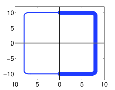
Figure 3: Contour $\Gamma$ used for counting of eigenvalues. Due to the symmetry of the Evans function, the computation was restricted to the thick contour in the right-half plane.

The presence of unstable eigenvalues is detected by contour integration using the argument principle, similarly as in [54], for $j$’s restricted by Proposition 34. The algorithm adaptively calculates the argument of the Evans function $E_{j}(\lambda)$ along an approximately rectangular contour $\Gamma$ which encloses a bounded region in $\mathbb{R}^{2}$. The region is pictured on Fig. 3. Note that Proposition 6 allows us to confine the integration to the right half plane (the total argument change is twice as large) and also reduces the set of $j$’s for which the calculation is necessary to positive values. Moreover, Proposition 37 restricts the location of unstable eigenvalues to a vertical strip. Naturally, it is not possible to perform numerical calculations without imposing also some vertical bound for the region enclosed by the contour. The vertical bound in the implementation is chosen is such a way that the behavior of the stable eigenvalues becomes predictable. We justified that all the unstable eigenvalues are included a posteriori by examining the Krein signature of eigenvalues.

Stable eigenvalues on the imaginary axis are, thanks to the symmetry of the Evans function, zeros of the real-valued function $E(\lambda)$. Hence one can plot that real function and determine the location and multiplicity of its zeros within a finite interval. In the actual implementation this is done automatically — one first interpolates the real function by a cubic spline and then uses the Newton method for locating zeros. In a small neighborhood of a possible double zero, a very fine mesh was used to resolve any ambiguity.

The total number of eigenvalues of $E_{j}(\lambda)$ enclosed in the region is then determined by the difference $n_{su}=n_{s+u}-n_{s}$ between the total number of eigenvalues inside $\Gamma$,

$$n_{s+u}=\frac{1}{2\pi i}\oint_{\Gamma}\frac{E_{j}^{\prime}(\lambda)}{E_{j}(\lambda)}d\lambda=\frac{1}{2\pi i}\oint_{\Gamma}\mbox{d arg}\,(E_{j}(\lambda))$$

and the number of (stable) eigenvalues $n_{s}$ on the imaginary axis, including their algebraic multiplicity. If $n_{su}$ is not equal to zero it must by Proposition 6 be an even positive integer and corresponds to twice the number of pairs of stable and unstable eigenvalues ($\lambda,\overline{\lambda}$) enclosed within $\Gamma$.

The precise location of unstable eigenvalues can be theoretically determined by the generalized argument principle. Higher moments

$$s_{k}=\sum\lambda_{i}^{k}=\frac{1}{2\pi i}\oint_{\Gamma}\lambda^{k}\frac{E_{j}^{\prime}(\lambda)}{E_{j}(\lambda)}d\lambda$$ (52)

give the sum of $k$-th powers of positions of all eigenvalues enclosed by $\Gamma$. Given the approximate location of eigenvalues on imaginary axis and number of eigenvalues off the axis, the problem reduces to solving a set of nonlinear equations. This is particularly efficient in the case $n_{su}=2$, where only $s_{1}$ is necessary. Unfortunately, even in this case, the numerical error involved can be significant, with a major contribution coming from a finite difference approximation of $E_{j}^{\prime}(\lambda)$. Therefore the obtained values are considered only approximate. The calculated location is further used to construct a smaller contour $\Gamma_{s}$ which lies solely in the right-half plane and encloses only a single eigenvalue. The presence of a zero of $E_{j}(\lambda)$ inside a smaller contour is again justified by the argument principle. Its location is then determined by the generalized argument principle. This process can be repeated a few times until a desired precision is attained. In the implementation the threshold for a precision was set up to be $10^{-3}$.

Note that this method of locating eigenvalues does not allow one to calculate the eigenfunction directly; for that another method must be used.

7.2 Numerical uses of Krein signature

Here we show how the Krein signature serves to provide evidence that no unstable eigenvalues are missed in the numerical computations. Moreover we suggest a very efficient numerical algorithm based on the theory in Section 6. Finally, we discuss an approach that does not require homotopy and avoids path-following completely.

In our numerical approach we consider the linearized eigenvalue problem for a large range of the parameter $\mu$, continuously connecting the linearized eigenvalue problem about a vortex solution to a linearized eigenvalue problem about a trivial solution. (See [14] for a similar approach). The latter problem has only purely imaginary eigenvalues, and their Krein signatures were determined in Section 6.2. We plot the location of all imaginary eigenvalues in a bounded interval on the imaginary axis which contains the continuation of all negative-signature eigenvalues for the whole range of $\mu$ considered ($\mu\in(m+1,35)$). By calculating the Evans function on the contour $\Gamma$ and on an appropriate portion of the imaginary axis, we indirectly track signature changes using the theory of Section 6, and can thus infer restrictions on possible departures of eigenvalues from the imaginary axis. This tracking process provides strong evidence that there are no unstable eigenvalues other than the ones we find.

For a significant reduction in computational effort, we propose a new numerical method that avoids the computation of contour integrals for Evans functions. To identify all unstable eigenvalues, it is only necessary to perform the following calculations:

• evaluate the Evans function on the imaginary axis close to zero to detect any eigenvalues crossing zero;

• follow the eigenvalue branches starting at negative Krein signature eigenvalues at the reference value of the continuation parameter (in our case start at $\mu=m+1$ and follow a total of $2m-1$ different branches), to detect any collision with positive Krein signature eigenvalues;

• follow any branches of eigenvalues that bifurcate into the complex plane.

We emphasize that the theory presented in Section 6 justifies that no unstable eigenvalues can be left out. No contour integration is necessary at all since one can just use a path-following algorithm (a boundary-value solver). Moreover, global analyticity of the Evans function is not needed, since only zeroes of the real Evans function on the imaginary axis need to be found initially, and one may use a continuation algorithm [27, 61] to track them.

A negative feature of the homotopy technique is that it has a large overhead if one is interested in only a small set of values of the parameter. Therefore we examine ways of avoiding this overhead by directly evaluating the Krein signature of a given eigenvalue on the imaginary axis. This is not feasible with the approach of evaluating Evans functions using exterior products, since the eigenfunction is unavailable and it must be calculated separately by a different method. On the other hand, the restriction of the Evans function to the imaginary axis is a real function. This means that only a continuous representation of the Evans function is required and problems of rapid growth and numerical dependence are much less severe. By consequence, it is not necessary to use exterior products to evaluate the Evans function, and it can be evaluated either (i) by calculating a relevant Wronskian of solutions to the linear eigenvalue equations which makes it easy to compute the eigenfunction, or (ii) one can use a simple continuation algorithm proposed by Sandstede [27]. By either of these methods, it is possible to evaluate the Krein signature directly, which then allows one to determine the number of unstable eigenvalues.

Then for an eigenvalue problem of the form $JLu=\lambda u$ the following method may be used. First, determine (somehow, by using oscillation theory, for example) the number $n_{total}$ of negative eigenvalues of $L$. If the number is zero, there are no unstable eigenvalues of $JL$. If $n_{total}>0$, the number gives the total number $n_{u}$ of pairs of unstable eigenvalues of $JL$ plus the number $n_{s}$ of stable eigenvalues with negative Krein signature [39, 40, 56] (also see [25]). If the present method (the Evans function) detects a number of pairs of eigenvalues off the imaginary axis $n_{u}=n_{total}$, there are no other unstable eigenvalues. If $n_{u}<n_{total}$, perform a calculation of the Krein signature for eigenvalues on the imaginary axis. If $n_{u}+n_{s}=n_{total}$ there are no other unstable eigenvalues, otherwise, increase the area of search and repeat the whole process.

7.3 Singly-quantized vortices $m=1$

Similarily as in [18, 37, 60, 68] we found singly-quantized vortex, $m=1$, to be spectrally stable for all values of the parameter $\mu$ investigated, $\mu\in(m+1,35)$, corresponding to number of particles $N\in(0,10^{6})$ for the data for   ²³${}_{\rule{0.0pt}{5.25pt}}$Na given in Section 2. By Propositions 34, 3 and 6 it suffices to study only $j=1$. For illustrative purposes the location of the stable eigenvalues ($\mu$ vs. $\mathop{\rm Im}\nolimits\lambda$) for $j=0,1,2,3$, is plotted in Fig. 4. For the sake of clarity only eigenvalues with $|\mathop{\rm Im}\nolimits\lambda|<5$ are shown.

For small values of $\mu$, close to $\mu_{0}=m+1$, the eigenvalues are close to the eigenvalues of the reduced uncoupled linear problem neglecting the $|w|^{2}$ dependence. As $\mu$ increases, certain eigenvalues remain constant: a double eigenvalue $\lambda=0$ and simple eigenvalues $\lambda=\pm 2i$ for $j=0$ and simple eigenvalues $\lambda=\pm i$ for $j=1$. These eigenvalues originate in the symmetries and boosts of the Gross-Pitaevskii equation and are present for every $m$ (see the Appendix).

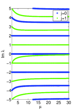
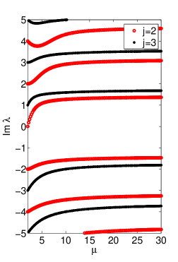
Figure 4: Stable eigenvalues of the linearization about a singly-quantized ($m=1$) vortex solution, $\mu\in(m+1,30)$: the eigenvalues corresponding to modes $j=0,1$ (left panel) and $j=2,3$ (right panel).

7.4 Multi-quantized vortices $m\geq 2$

The eigenvalue diagrams for multi-quantized vortices with $m=2$ show more complexity. The radial vortex profile for $\mu\approx 35$ is illustrated in Fig. 1.

In the case $m=2$ the possible unstable eigenvalues may appear for $|j|=1,2,3$. The modes $j=0$ and $j=1$ demonstrate the same features as in the case of the singly-quantized vortex with the same constant eigenvalues: a double eigenvalue $\lambda=0$ and simple eigenvalues $\lambda=\pm 2i$ for $j=0$ and simple eigenvalues $\lambda=\pm i$ for $j=1$ (see Fig. 5 (a)).

A different behavior appears for modes $j=2$ and $j=3$, as shown on Fig. 5 (b) and Fig. 7. For $j=3$ there are no unstable eigenvalues present and the stable eigenvalues do not collide but rather diverge from each other when they approach each other. Collisions do occur for $j=2$ and cause instability. A collision of two stable purely imaginary eigenvalues produces a pair of stable and unstable complex eigenvalues symmetric with respect to the imaginary axis. After an increase of $\mu$ these two eigenvalues return to the imaginary axis and split to two purely imaginary eigenvalues as illustrated in Fig. 6. This “collision – split – collision” process (“bubbles of instability” [50]) repeats regularly for the whole range of $\mu$ studied.

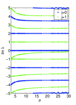
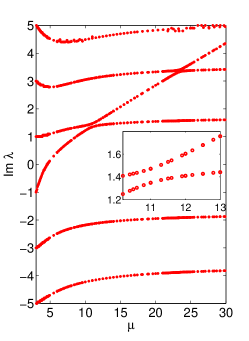
Figure 5: Stable eigenvalues of the linearization about a multi-quantized vortex solution, $m=2$, $\mu\in(m+1,35)$: $j=0,1$ (left panel) and $j=3$ (right panel), with a detail of an avoided eigenvalue collision on the inset.

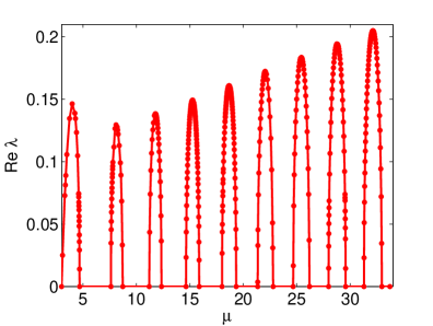
Figure 6: Stable and unstable eigenvalues of the linearization about a multi-quantized vortex solution, $m=2$, $\mu\in(m+1,35)$, corresponding to the mode $j=2$.

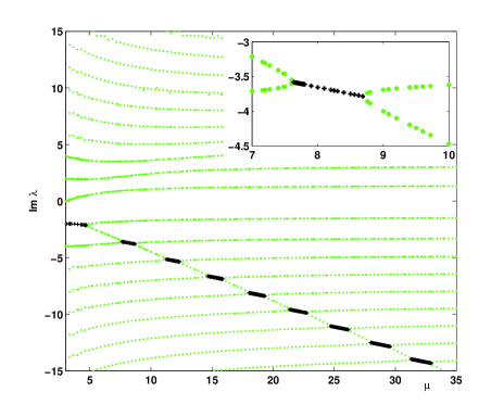
Figure 7: Imaginary part of stable (light) and unstable (dark) eigenvalues of the linearization about a multi-quantized vortex solution, $m=2$, $\mu\in(m+1,35)$, corresponding to mode $j=2$. A detail of a bubble of instability on the inset.

This behavior is caused by the presence of a single eigenvalue with negative Krein signature [50, 68]. The imaginary part of this eigenvalue is decreasing with increasing $\mu$, and on its way it encounters eigenvalues with the opposite signature. After each collision the eigenvalues split off the imaginary axis and become eigenvalue pairs with zero Krein signature symmetric relative to the imaginary axis. Reversibility of this process suggests that the eigenvalues come back to the imaginary axis and the process repeats itself (for a larger parameter $\mu$). This indicates a surprising thing: transitions to instability for larger $\mu$ may happen at a large frequency ($\mbox{Im}\,\lambda$ large), and therefore there is no hope to confine the imaginary parts of unstable eigenvalues to a finite interval independent of $\mu$. The behavior of the eigenvalues demonstrates strong agreement with [60]. This is also consistent with the results of Seiringer [65] where he proved that for any $m\geq 1$ for large enough $\mu$ the vortex becomes energetically unstable in the sense that it cannot be a global minimizer of the energy and is subject to symmetry breaking. Also note, that the maximum real part of unstable eigenvalues grows very slowly with growing parameter $\mu$. The maximum of the real part is much smaller than the bound we were able to obtain in Proposition 37.

In the case $j=3$ the eigenvalues have the same Krein signature and therefore they cannot split off the imaginary axis The eigenvalue which originates at $\lambda=-i$ for $\mu=3$ has negative signature at first, but after it crosses zero for $\mu$ close to 5, it changes its signature to positive according to Corollary 2. Then all eigenvalues have the same signature, making splitting impossible. Instead, eigenvalues repel each other upon approach, as expected by [50].

7.5 Further results

The presence of exponential instability was also checked by direct simulations. First, an approximate eigenvector was obtained by Galerkin approximation [18] and then the Strang-splitting scheme [6] was used for time evolution. The initial perturbation of a vortex solution by an approximated eigenvector showed a good agreement with the expected exponential growth.

For the case $m=3$, we performed similar computations but omit details for brevity. There are more eigenvalues of negative Krein signature, and overlapping bubbles of instability. See [60] for the analog of Fig. 6 in this case.

Finally, it would be plausible to describe the asymptotics of the eigenvalues as $\mu\rightarrow\infty$ when the condensate approaches the Thomas-Fermi regime. We were only able to study the asymptotic behavior of purely imaginary eigenvalues numerically by plotting a loglog plot of the first order differences of $\lambda(\mu)$. We observed a clear linear trend implying an algebraic approach to a limit. Our numerical results agree with the recent analytical results in [57] for stability of vortex solutions in the limiting Thomas-Fermi regime (see also [17] for stability of ground states).

The approximate behavior of eigenvalues with a small imaginary part for $m=1$, $j=1,2$, and $m=2$, $j=2,3$, is presented in Table 1. For most eigenvalues, the asymptotic behavior as $\mu\gg 1$ is well approximated by

$$\lambda(\mu)=b-\frac{c}{\mu}.$$

On the other hand, certain eigenvalues show different rate of convergence clearly distinct from $(-\mu^{-1})$, but we do not have any explanation of this phenomena.

$m=1$	$j=1$	$\lambda_{0}=-3i$	$-i\lambda(\mu)=-2.64-1.24\,\mu^{-1.02}$
		$\lambda_{0}=-i$	$-i\lambda(\mu)=0.01-1.48\,\mu^{-0.80}$
		$\lambda_{0}=3i$	$-i\lambda(\mu)=2.73-0.17\,\mu^{-0.14}$
	$j=2$	$\lambda_{0}=-2i$	$-i\lambda(\mu)=-1.41-1.82\,\mu^{-1.04}$
		$\lambda_{0}=0$	$-i\lambda(\mu)=1.41-1.61\,\mu^{-1.04}$
		$\lambda_{0}=2i$	$-i\lambda(\mu)=3.16-2.43\,\mu^{-1.02}$
$m=2$	$j=2$	$\lambda_{0}=-4i$	$-i\lambda(\mu)=-1.41-2.69\,\mu^{-0.96}$
		$\lambda_{0}=0$	$-i\lambda(\mu)=1.38-7.96\,\mu^{-1.39}$
		$\lambda_{0}=2i$	$-i\lambda(\mu)=3.11-27.66\,\mu^{-1.59}$
	$j=3$	$\lambda_{0}=-3i$	$-i\lambda(\mu)=-1.74-5.14\,\mu^{-1.06}$
		$\lambda_{0}=-i$	$-i\lambda(\mu)=1.73-3.97\,\mu^{-1.02}$
		$\lambda_{0}=i$	$-i\lambda(\mu)=3.61-5.30\,\mu^{-0.97}$

Table 1: Approximate asymptotic behavior of eigenvalues for $m=1,2$.

Appendix: Symmetries and eigenvalues

The symmetries of the Gross-Pitaevskii equation and its linearization imply the presence of a special set of eigenvalues.

Phase symmetries. For any $m$,

$$\lambda=0\quad\mbox{(for $j=0$)}$$

is a constant double eigenvalue for all $\mu\geq\mu_{0}$. Its multiplicity comes from the symmetry of the Gross-Pitaevskii equation under a phase change (this generates an eigenvector) and under a change of standing-wave frequency (this generates a generalized eigenvector). A detailed discussion on these two symmetries and their implications for spectra is given in [54].

GGV boost. Due to the presence of the harmonic potential, the other usual invariants of the nonlinear Schrödinger equation—spatial translations—do not apply. Similarly, one cannot perform the typical Galilean boost. Instead, one can apply a boost for quadratic potentials that was described by García-Ripoll et al. [19]. This particular boost transforms any solution $\Psi(\mbox{\boldmath$r$\unboldmath},t)$ ($\mbox{\boldmath$r$\unboldmath}=(x,y)$) to a new solution of the form

$$\Psi_{R}(\mbox{\boldmath$r$\unboldmath},t)=\Psi(\mbox{\boldmath$r$\unboldmath}-R(t),t)\exp(i\mbox{\boldmath$\theta$\unboldmath}(\mbox{\boldmath$r$\unboldmath},t))\,,$$ (53)

where $R(t)$ is the path of a classical particle moving in the potential well. For the harmonic potential $V(\mbox{\boldmath$r$\unboldmath})=\frac{1}{2}\mbox{\boldmath$r$\unboldmath}^{2}$, this requires simply $R_{tt}=-R$, so that each component of $R(t)$ can be any linear combination of $\cos t$ and $\sin t$. According to [19], $\theta$ is given up to a constant by $\mbox{\boldmath$\theta$\unboldmath}(\mbox{\boldmath$r$\unboldmath},t)=\mbox{\boldmath$r$\unboldmath}\cdot R_{t}$.

As discussed in [54], any one-parameter family $u_{\tau}$ of solutions to (6) gives rise to a solution of the corresponding equation linearized about $u_{0}$, given by

$$\tilde{u}:=\partial_{\tau}u_{\tau}|_{\tau=0}\,.$$

In the case of the GGV boost (53), setting $R(t)=\tau(\cos t,\sin t)^{T}$ gives $\mbox{\boldmath$\theta$\unboldmath}(r,\theta,t)=\tau r\cos(\theta-t)$. Then $u_{\tau}$ is given by (53) with $\Psi(\mbox{\boldmath$r$\unboldmath},t)=\psi(t,r,\theta)$ as given by (10) with $w(r)$ satisfying (11). Hence

$$\tilde{u}=\binom{\cos t}{\sin t}\cdot{\mathbf{\nabla}}\psi(t,r,\theta)+ir\cos(\theta-t)\psi(t,r,\theta)\,,$$

which can be also written as

$$\tilde{u}=e^{-i\mu t}e^{im\theta}\left[w^{\prime}(r)\cos(\theta-t)+i\frac{mw}{r}\sin(t-\theta)+irw\cos(t-\theta)\right]\,.$$

The vector $\tilde{\Psi}=(\mathop{\rm Re}\nolimits\tilde{u},\mathop{\rm Im}\nolimits\tilde{u})^{T}$ then satisfies the linearized equations (20) and has the form

$$e^{\mu t}\tilde{\Psi} = \binom{\cos m\theta}{\sin m\theta}\binom{\cos\theta}{\sin\theta}\cdot\binom{\cos t}{\sin t}w^{\prime}(r)$$

$$+\binom{-\sin m\theta}{\cos m\theta}\!\left[-\binom{\cos\theta}{\sin\theta}\!\cdot\!\binom{-\sin t}{\cos t}\frac{mw(r)}{r}+\binom{\cos\theta}{\sin\theta}\!\cdot\!\binom{\cos t}{\sin t}rw(r)\right].$$

In the decoupling to Fourier modes this solution yields a solution to the system (29)–(30) for $j=1$, $\lambda=i$ and

$$y_{+}=\frac{1}{2}\left[w^{\prime}(r)-\frac{mw(r)}{r}+rw(r)\right]\,,\quad y_{-}=\frac{1}{2}\left[w^{\prime}(r)+\frac{mw(r)}{r}-rw(r)\right]\,.$$

The similar solution can be also obtained for $\lambda=-i$:

$$y_{+}=\frac{1}{2}\left[w^{\prime}(r)-\frac{mw(r)}{r}-rw(r)\right]\,,\quad y_{-}=\frac{1}{2}\left[w^{\prime}(r)+\frac{mw(r)}{r}+rw(r)\right]\,.$$

Therefore the GGV boost implies the existence of the eigenvalues (for any $m$)

$$\lambda=\pm i\quad\mbox{(for $j=1$).}$$

Breather boost. Finally, we describe the source of the presence of the eigenvalues

$$\lambda=\pm 2i\quad\mbox{(for $j=0$)},$$

which appear for every $m\geq 1$ and $\mu\geq\mu_{0}$. These eigenvalues corresponds to a “breathing” symmetry of the Gross-Pitaevskii equation in $2+1$ dimensions, as explained by Pitaevskii and Rosch in [59]. Here we provide a somewhat different perspective, showing that the symmetry corresponds to the Talanov lens transformation via an exact transformation to the cubic Schrödinger equation. Rybin et al. [64] noted that the radially symmetric Gross-Pitaevskii equation in 2+1 dimensions transforms exactly to the cubic Schrödinger equation without potential, according to a transformation described originally by Niederer [52] for the linear Schrödinger equation. More generally, they noted that this transformation works in any dimension as long as the nonlinearity is critical, of the form $|u|^{4/n}u$ in $n$ space dimensions. This symmetry was used by Carles [7] to study various mathematical aspects of the Gross-Pitaevskii equation.

By transforming from GP to cubic Schrödinger, using a Talanov lens transformation [70], and transforming back, one can get a self-transformation of GP (see also [21]). The symmetry that we will describe is somewhat more general, and works as follows. Suppose that $v(x,t)$ is any solution of the equation

$${\rm i}\partial_{t}v+\frac{1}{2}\Delta v-\frac{1}{2}{\omega^{2}}|x|^{2}v-\lambda|v|^{p}v=0$$ (54)

where $t\in\mathbb{R}$ and $x\in\mathbb{R}^{n}$. Let

$$u(t,x)=a{\rm e}^{-{\rm i}b|x|^{2}/2}v(cx,\tau)$$ (55)

where $a$, $b$, $c$ and $\tau$ are functions of time $t$. Then we find that

$${\rm i}\partial_{t}u+\frac{1}{2}\Delta u-\frac{1}{2}{\nu^{2}}|x|^{2}u-\gamma|u|^{p}u=0,$$ (56)

provided that $b$ and $c$ satisfy

$$b^{\prime}-b^{2}+{\omega^{2}}c^{4}={\nu^{2}},\quad c^{\prime}=bc,$$ (57)

and

$$a=c^{n/2},\quad\tau^{\prime}=c^{2},\quad\gamma=\lambda c^{2-np/2}.$$ (58)

Of course, $b=0$, $c=1$, always works with ${\nu^{2}}={\omega^{2}}$.

The symmetry is most interesting when the nonlinearity is critical, meaning $p=4/n$. Then $\gamma=\lambda$. In 2+1 dimensions this corresponds to the cubic nonlinearity. For ${\omega^{2}}={\nu^{2}}=0$ we recover the well-known Talanov lens transformation for the critical Schrödinger equation:

$$b=\frac{b_{0}}{1-b_{0}t},\quad c=\frac{c_{0}}{1-b_{0}t},\quad\tau=\frac{c_{0}^{2}t}{1-b_{0}t}.$$ (59)

With ${\omega^{2}}=0$ and constant ${\nu^{2}}>0$ we get the transformation from the critical Schrödinger equation to GP as described by Rybin et al. [64] and Carles [7]:

$$b=\nu\tan\nu t,\quad c=\frac{1}{\cos\nu t},\quad\tau=\frac{\tan\nu t}{\nu}.$$ (60)

In the other direction with constant ${\omega^{2}}>0$ and ${\nu^{2}}=0$ we get [7]:

$$b=-\frac{{\omega^{2}}t}{1+{\omega^{2}}t^{2}},\quad c=\frac{1}{\sqrt{1+{\omega^{2}}t^{2}}},\quad\tau=\frac{\arctan\omega t}{\omega}.$$ (61)

The consequences of this transformation for the Gross-Pitaevskii equation in 2+1 dimensions are striking. From any solution of (54), one gets from (55) a solution obtained by a breather boost — a time-periodic dilation of space with an appropriate radial phase adjustment. See [59] for more discussion and a relation to representations of the group SO(2,1).

A short calculation shows that this transformation corresponds to the eigenvalues $\pm 2i$ of the normalized linearized equations (29)–(30). The relation to these eigenvalues can be seen also from a simple consideration, that this self-transformation produces small oscillations at exactly twice the trap frequency for classical oscillations in the harmonic potential $\frac{1}{2}{\omega^{2}}|x|^{2}$. The exact formulae for this breathing boost also show that breathing oscillations need not be small. Also note that a breather boost can be applied to any solution, not only standing waves.

References

- [1] M. Abramowitz, I. A. Stegun. Handbook of mathematical functions with formulas, graphs, and mathematical tables. National Bureau of Standards Applied Mathematics Series 55 (1964).
- [2] A. Aftalion, Q. Du. Vortices in a rotating Bose-Einstein condensate: critical angular velocities and energy diagrams in the Thomas-Fermi regime. Phys.Rev. A, 64 (2001), 063603.
- [3] J. Alexander, R. Gardner, C. K. R. T. Jones. A topological invariant arising in the stability analysis of traveling waves. J. Reine Angew. Math., 410 (1990), 167–212.
- [4] E. L. Allgower, K. Georg. Numerical Continuation Methods: An Introduction. Series in Computational Mathematics 13 (Springer, 1990).
- [5] M. H. Anderson, J. R. Ensher, M. R. Matthews, C. E. Wieman, E. A. Cornell. Observation of Bose-Einstein condensation in a dilute atomic vapor. Science, 269 (1995), 198–201.
- [6] W. Bao, D. Jaksch, P. A. Markowich. Numerical solution of the Gross-Pitaevskii equation for Bose-Einstein condensation. J Comp. Phys., 187 (2003), 318–342.
- [7] R. Carles. Critical nonlinear Schrödinger equations with and without harmonic potential, Math. Mod. Meth. Appl. Sci. 12 (2002) 1513–1523.
- [8] Y. Castin, R. Dum. Bose-Einstein condensates with vortices in rotating traps. Eur. Phys. J. D, 7 (1999), 399–412.
- [9] M. Chugunova, D. Pelinovsky. Count of eigenvalues in the generalized eigenvalue problem, J. Math. Phys. 51 (2010), 052901.
- [10] W. A. Coppel. Stability and Asymptotic Behavior of Differential Equations (D.C. Heath and Co., 1965).
- [11] M. G. Crandall, P. H. Rabinowitz. Bifurcation, perturbation of simple eigenvalues and linearized stability. Arch. Rational Mech. Anal., 52 (1973), 161–180.
- [12] F. Dalfovo, S. Giorgini, L. P. Pitaevskii, S. Stringari. Theory of Bose-Einstein condensation in trapped gases. Rev. Mod. Phys. 71 (1999), no. 3, 463–512.
- [13] K. B. Davis, M. O. Mewes, M. R. Andrews, N. J. van Druten, D. S. Durfee, D. M. Kurn, W. Ketterle. Bose-Einstein condensation in a gas of sodium atoms. Phys. Rev. Lett., 75 (1995), 3969–3973.
- [14] M. Edwards, R. J. Dodd, C. W. Clark, K. Burnett. Zero-temperature, mean-field theory of atomic Bose-Einstein condensates. J. Res. Natl. Inst. Stand. Technol. 101 (1996), 553.
- [15] J. W. Evans. Nerve axon equations. IV. The stable and unstable impulse. Indiana Univ. Math. J. 24 (1975), 1169–1190.
- [16] A. L. Fetter, A. A. Svidzinsky. Vortices in a trapped dilute Bose-Einstein condensate. J. Phys. Condens. Matter, 13 (2001) no. 12, R135.
- [17] C. Gallo, D. Pelinovsky. Eigenvalues of a nonlinear ground state in the Thomas-Fermi approximation, J. Math. Anal. Appl. 355 (2009) 495–526.
- [18] J. J. García-Ripoll, V. M. Pérez-García. Stability of vortices in inhomogeneous Bose condensates subject to rotation: A three-dimensional analysis. Phys. Rev. A, 60 (1999), no. 6, 4864–4874.
- [19] J. J. García-Ripoll, V. M. Pérez-García , V. Vekslerchik. Construction of exact solutions by spatial translations in inhomogeneous nonlinear Schrödinger equations. Phys. Rev. E 64 (2001), 056602.
- [20] I. M. Gelfand and V. B. Lidskiĭ. On the structure of the regions of stability of linear canonical systems of differential equations with periodic coefficients, Amer. Math. Soc. Transl. (2) 8 (1958), 143–181.
- [21] P. K. Ghosh. Explosion-implosion duality in the Bose-Einstein condensation. Phys. Lett. A 308 (2003), no. 5, 411–416.
- [22] I. C. Gohberg, M. G. Krein. Introduction to the theory of linear nonselfadjoint operators. Transactions Mathematical Monographs, no. 18 (American Mathematical Society, 1969).
- [23] M. Grillakis. Analysis of the linearization around a critical point of an infinite dimensional Hamiltonian system. Comm. Pure Appl. Math. 43 (1990), 299–333.
- [24] M. Grillakis, J. Shatah, W. Strauss. Stability theory of solitary waves in the presence of symmetry. I. J. Funct. Anal. 74 (1987), no. 1, 160–197.
- [25] K. F. Gurski, R. Kollár, R. L. Pego. Slow damping of internal waves in a stably stratified fluid. Proc. R. Soc. Lond. A 460 (2004), 977–994.
- [26] M. Haragus, T. Kapitula. On the spectra of periodic waves for infinite-dimensional Hamiltonian systems Phys. D 237 (2008) no.20, 2649–2671.
- [27] J. Humpherys, B. Sandstede, K. Zumbrun. Efficient computation of analytic bases in Evans function analysis of large systems. Numer. Math. 103 (2006), no. 4, 631–642.
- [28] J. Humpherys, K. Zumbrun. An efficient shooting algorithm for Evans function calculations in large systems. Phys. D 220 (2006), no. 2, 116–126.
- [29] J. Iaia, H. Warchall. Nonradial solutions of a semilinear elliptic equation in two dimensions. J.Diff. Eq. 119 (1995), no. 2, 533–558.
- [30] R. Ignat, V. Millot. The critical velocity for vortex existence in a two-dimensional rotating Bose-Einstein condensate. J. Funct. Anal. 233 (2006), no. 1, 260–306.
- [31] T. Isoshima, K. Machida. Vortex stabilization in dilute Bose-Einstein condensate under rotation. J. Phys. Soc. Jpn. 68 (1999), 487–492.
- [32] T. Isoshima, K. Machida. Vortex stabilization in Bose-Einstein condensate of alkali-metal atom gas. Phys. Rev. A, 59 (1999), 2203–2212.
- [33] R. K. Jackson, M. I. Weinstein. Geometric analysis of bifurcation and symmetry breaking in a Gross-Pitaevskii equation. J. Statist. Phys. 116 (2004), no. 1–4, 881–905.
- [34] T. Kapitula. The Krein signature, Krein eigenvalues, and the Krein Oscillation Theorem, Indiana Univ. Math. J., to appear (2009).
- [35] T. Kapitula, P. G. Kevrekidis. Bose-Einstein condensates in the presence of a magnetic trap and optical lattice. Chaos 15 (2005), no. 3, 037114.
- [36] T. Kapitula, P. G. Kevrekidis. Bose-Einstein condensates in the presence of a magnetic trap and optical lattice: two-mode approximation. Nonlinearity 18 (2005), no. 6, 2491–2512
- [37] T. Kapitula, P. G. Kevrekidis, R. Carretero-González. Rotating matter waves in Bose-Einstein condensates. Phys. D 233 (2007), no. 2, 112–137.
- [38] T. Kapitula, P. G. Kevrekidis, D. J. Frantzeskakis. Disk-shaped Bose-Einstein condensates in the presence of an harmonic trap and an optical lattice. Chaos 18 (2008), no. 2, 023101
- [39] T. Kapitula, P. G. Kevrekidis, B. Sandstede. Counting eigenvalues via the Krein signature in infinite-dimensional Hamiltonian systems. Physica D 195 (2004), no. 3–4, 263–282.
- [40] T. Kapitula, P. G. Kevrekidis, B. Sandstede. Addenum: Counting eigenvalues via the Krein signature in infinite-dimensional Hamiltonian systems. Physica D 201 (2005), no. 1–2, 199–201.
- [41] T. Kato. Perturbation Theory for Linear Operators (Springer, 1976).
- [42] P. G. Kevrekidis, D. J. Frantzeskakis, R. Carretero-González eds. Emergent Nonlinear Phenomena in Bose-Einstein Condensates (Springer, 2008).
- [43] P. G. Kevrekidis, D. J. Frantzeskakis, B. A. Malomed, A. R. Bishop, I. G. Kevrekidis. Dark-in-bright solitons in Bose-Einstein condensates with attractive interactions. New Journal of Physics 5 (2003), 64.1–64.17.
- [44] R. Kollár. Existence and stability of vortex solutions of certain nonlinear Schrödinger equations. PhD thesis. University of Maryland, College Park (2004).
- [45] E. H. Lieb, R. Seiringer. Proof of Bose-Einstein condensation for dilute trapped gases. Phys. Rev. Lett. 88 (2002), 170409.
- [46] E. H. Lieb, R. Seiringer, J. P. Solovej, J. Yngvanson. The ground state of the Bose gas. Current developments in mathematics, 131–178 (Intl. Press, 2002).
- [47] E. H. Lieb, R. Seiringer, J. Yngvanson. A rigorous derivation of the Gross-Pitaevskii energy functional for a two-dimensional Bose gas. Comm. Math. Phys., 224 (2001), no.1, 17–31.
- [48] E. H. Lieb, R. Seiringer, J. P. Solovej, J. Yngvason. The Mathematics of the Bose Gas and its Condensation. Oberwolfach Seminars, Vol. 34 (Birkhäuser, 2005).
- [49] E. H. Lieb, R. Seiringer. Derivation of the Gross-Pitaevskii equation for rotating Bose gases. Comm. Math. Phys. 264 (2006), no. 2, 505–537.
- [50] R. MacKay. Stability of equilibria of Hamiltonian systems. In: Hamiltonian Dynamical Systems (R. MacKay and J. Meiss, eds.), 137–153 (Adam Hilger, 1987).
- [51] J.C. Neu. Vortices in complex scalar fields. Physica D 43 (1990), 385–406.
- [52] U. Niederer. The maximal kinematical invariance groups of Schrödinger equations with arbitrary potentials, Helv. Phys. Acta 47 (1974) 167–172.
- [53] L. Nirenberg. Topics in Nonlinear Functional Analysis (Amer. Math. Soc., Providence, 2001).
- [54] R. L. Pego, H. A. Warchall. Spectrally stable encapsulated vortices for nonlinear Schrödinger equations. J. Nonlinear Sci.12 (2002), 347—394.
- [55] R. L. Pego, M. I. Weinstein. Eigenvalues, and instabilities of solitary waves. Phil. Trans. Roy. Soc. London A 340 (1992), 47–94.
- [56] D. E. Pelinovsky. Inertia law for spectral stability of solitary waves in coupled nonlinear Schrödinger equations. Proc. R. Soc. Lond. Ser. A 461 (2005), no. 2055, 783–812.
- [57] D. E. Pelinovsky, P. G. Kevrekidis. Variational approximations of trapped vortices in the large-density limit, submitted to Nonlinearity (2010).
- [58] C. J. Pethick, H. Smith. Bose-Einstein Condensates in Dilute Gases (Cambridge Press, 2002).
- [59] L. P. Pitaevskii, A. Rosch. Breathing modes and hidden symmetry of trapped atoms in two dimensions, Phys. Rev. A 55 (1997), no. 2, R853.
- [60] H. Pu, C. K. Law, J. H. Eberly, N. P. Bigelow. Coherent disintegration and stability of vortices in trapped Bose condensates. Phys. Rev. A 59 (1999), 1533.
- [61] J. D. M. Rademacher, B. Sandstede, A. Scheel. Computing absolute and essential spectra using continuation. Phys. D 229 (2007), no. 2, 166–183.
- [62] M. Reed, B. Simon. Methods of Modern Mathematical Physics I: Functional Analysis (Academic Press Inc., 1972).
- [63] M. Reed, B. Simon. Methods of Modern Mathematical Physics IV: Analysis of Operators (Academic Press Inc., 1978).
- [64] A. V. Rybin, G. G. Varzugin, M. Lindberg, J. Timonen and R. K. Bullough. Similarity solutions and collapse in the attractive Gross-Pitaevskii equation. Phys. Rev. E 62 (2000) no.5, 6224.
- [65] R. Seiringer. Gross-Pitaevskii theory of the rotating Bose gas. Comm. Math. Phys., 229 (2002), 491–509.
- [66] T. P. Simula, S. M. M. Virtanen, M. M. Salomaa. Stability of multiquantum vortices in dilute Bose-Einstein condensates. Phys.Rev. A, 65 (2002), 033614.
- [67] D. V. Skryabin. Instabilities of vortices in a binary mixture of trapped Bose-Einstein condensates: Role of collective excitations with positive and negative energies. Phys. Rev. A 63 (2000), 013602.
- [68] D. V. Skryabin. Energy of internal modes of nonlinear waves and complex frequencies due to symmetry breaking. Phys. Rev. E 64 (2001), 055601.
- [69] J. Stoer, R. Bulirsch. Introduction to Numerical Analysis. 2nd ed. (Springer Verlag, 1993).
- [70] V. Talanov. Focusing of light in cubic media, J. Exp. Theo. Phys. Lett. 11 (1970), 199–201.
- [71] S. M. M. Virtanen, T. P. Simula, M. M. Salomaa. Structure and stability of vortices in dilute Bose-Einstein condensates at ultralow temperatures. Phys. Rev. Lett. 86 (2001), 2704–2707.
- [72] V. A. Yakubovich, V. M. Starzhinskii. Linear Differential Equations with Periodic Coefficients I (Halsted Press, 1975).