Construction of the surfaces with horizontal tangential planes at given points

Abstract

The problem of construction of the surfaces with given sets of the points with horizontal tangential planes is considered. Such considerations are of interest in the problem of computer simulations of the waved ocean surfaces.

1 Statement of the problem

1.1 Physical statement

Various problems of optical/acoustical monitoring of wavy water surface are related with simulations of the surfaces with given properties [1, 2, 3]. The example of it is the problem of construction of two-dimension surface having horizontal target planes at the given points (Luchinin A.G., 2003). Variants of solutions of this problem are presented in this article.

1.2 Mathematical formulation

The main problem A. Let $\mathfrak{M=}\left\{\mathbf{x}_{i},\ i=\overline{0,N}\right\}$ be the finite subset of the given open set $\Omega\subset R^{n}\emph{,}n\geq 1.$ Construct a function $F\left(\mathbf{x}\right)$ of the given class $\mathfrak{F}\in C^{1}\left(\Omega\right)$ possessing zero gradient $\nabla F\left(\mathbf{x}\right)=\mathbf{0}$ at all points of $\mathfrak{M}$ .

We study also the next specifications of the main problem:

B.

the values of the function at the points $\mathfrak{M}$ are given ($F\left(\mathbf{x}_{i}\right)=z_{i},\ i=\overline{0,N}$);

C.

gradient of the function takes zero values only in $\mathfrak{M}$.

It is clear that sets of the solutions of A-C are infinite. In general, solutions of the main problem A do not solve problems B,C. The main goal of the next research is to determine the existence of the solution of a problem in a given class of functions $\mathfrak{F}$.

2 Analytical approach

Let $\mathfrak{F}=C^{k}\left(\Omega\right)$, $1\leq k\leq\infty$. For this class of functions we can easily construct an analytic solution of the main problem. One of possible constructions is described below. Let $\left|\cdot\right|$ be Euclidean norm in $R^{n}$. Consider for every point $\mathbf{x}_{i}$ $\in\mathfrak{M}$ the open sphere

$$S_{i}\equiv\left\{\mathbf{x}:\left|\mathbf{x-x}_{i}\right|<r_{i}\right\}\subset\Omega$$

with the radius $r_{i}>0$ and center point $\mathbf{x}_{i}$. Let $a_{i}>1$, $c_{i}$ be arbitrary values, $\varphi_{i}\left(\cdot\right)\in C^{k}\left(R^{n}\right)$ be arbitrary functions such that $\varphi_{i}\left(\mathbf{0}\right)=1$, $\nabla\varphi_{i}\left(\mathbf{0}\right)=0$. Let

$$\chi_{i}\left(\mathbf{x}\right)\equiv\left\{\begin{array}[c]{ll}a_{i}^{\frac{\left|\mathbf{x}\right|^{2}}{\left|\mathbf{x}\right|^{2}-r_{i}^{2}}},&\left|\mathbf{x}\right|<r_{i},\\ 0,&\left|\mathbf{x}\right|\geq r_{i},\end{array}\right.$$ (3)

$$F\left(\mathbf{x}\right)={\displaystyle\sum\limits_{i=0}^{N}}c_{i}\chi_{i}\left(\mathbf{x-x}_{i}\right)\varphi_{i}\left(\mathbf{x-x}_{i}\right).$$ (4)

It easy to prove the following statements.

Proposition 1. For every set of sufficiently small values $r_{i}$ (such that $\mathbf{x}_{i}\notin$ $S_{j}$, $j\neq i$) and for any values $c_{i}$ the function (4) is a solution of the problem A. In addition, if

1. $c_{i}=z_{i},\ i=\overline{0,N}$, then (4) gives a solution of the problem B;

2. all spheres $S_{j}$ do not intersect, then (4) gives a solution of the problem C.

Proposition 2. Let $n=1$, $x_{0}<x_{1}<\ldots<x_{N}$ . Then under the conditions

$$r_{i}\leq\left|x_{i}-x_{i-1}\right|,~{}c_{i-1}c_{i}<0,\ i=\overline{1,N},$$

the function (4) gives a solution of the problem C.

The peculiarity of the described construction is the provided by multipliers $\chi_{i}\left(\mathbf{x}\right)$ finiteness of the terms of the sum (4); this provides zero values of gradient at the points of $\mathfrak{M}$. Note that using the corresponding values of gradients $\nabla\varphi_{i}\left(\mathbf{0}\right)$ we can assume these gradients not only zero but also any given, so we can use the construction (4) for solving of more complicated problems to construct of surfaces with given slopes at the given points.

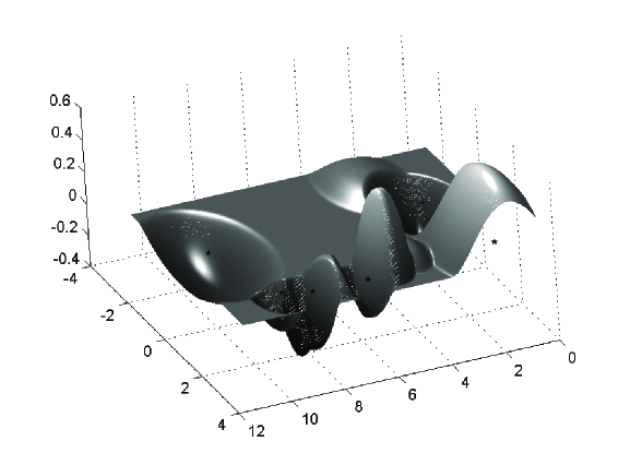
From physical point of view the solutions (4) can simulate only oscillation of too viscous liquid. An example of the numerical simulation by means of formula (4) for $a_{i}=e$, $\varphi_{i}\left(\mathbf{x}\right)\equiv 1$, $10$ random points $\mathfrak{M}$ and random coefficients $c_{i}$, is presented on Fig. 1.

Figure 1: The surface (4) for the set of $10$ random points marked on the graph by stars.

3 Spline approach

In this section we use splines of various types to solve problems A-C for $n=1,2$. Polynomial splines of the 4-th order (see sec. 3.1.1, 3.1.2) make it possible to solve problems A and B. As for the problem C then in the case $n=2$ spline approach is useless if only the set $\mathfrak{M}$ does not have the form of the product

$$\mathfrak{M}=X\times Y,\ \ \left\{\begin{array}[c]{l}X=\left\{x_{k}\right\},\ k=\overline{0,K},\\ Y=\left\{y_{l}\right\},\ \ l=\overline{0,L}.\end{array}\right.$$ (5)

But in the case $n=1$ the solution of the problem C can be found in the class of trigonometric splines (sec. 3.2.1).

3.1 Polynomial splines

3.1.1 One-dimensional problem ($n=1$)

Consider the following problem B: for given sets $a=x_{0}<x_{1}<\ldots<x_{N}=b$ and $\left\{z_{i},i=\overline{0,N},\right\}$ build a spline of the 4-th order $F\left(\cdot\right)\in C^{1}\left[a,b\right]$ such that

$$\left\{\begin{array}[c]{l}F\left(x\right)=s_{i}\left(x\right),\ x\in\left[x_{i-1},x_{i}\right],\ i=\overline{1,N},\\ s_{i}\left(x\right)\equiv a_{i}+b_{i}\left(x-x_{i}\right)+c_{i}\left(x-x_{i}\right)^{2}/2!+d_{i}\left(x-x_{i}\right)^{3}/3!+e_{i}\left(x-x_{i}\right)^{4}/4!,\\ F\left(x_{i-1}\right)=z_{i-1},\ \ \ F\left(x_{i}\right)=z_{i},\\ F^{\prime}\left(x_{i-1}\right)=0,\ \ F^{\prime}\left(x_{i}\right)=0.\end{array}\right.$$ (6)

Now we prove that such splines exist. We have for the coefficients of the spline

$$\left\{\begin{array}[c]{l}F\left(x_{i}\right)=a_{i}=z_{i},\\ F^{\prime}\left(x_{i}\right)=b_{i}=0,\\ F\left(x_{i-1}\right)=a_{i}+b_{i}\Delta x_{i}+c_{i}\Delta x_{i}^{2}/2+d_{i}\Delta x_{i}^{3}/6+e_{i}\Delta x_{i}^{4}/24=z_{i-1},\\ F^{\prime}\left(x_{i-1}\right)=b_{i}+c_{i}\Delta x_{i}+d_{i}\Delta x_{i}^{2}/2+e_{i}\Delta x_{i}^{3}/6=0,\\ \Delta x_{i}\equiv x_{i-1}-x_{i},\ i=\overline{1,N}.\end{array}\right.$$

So we obtain the equations

$$\left\{\begin{array}[c]{l}c_{i}=-d_{i}\Delta x_{i}/2-e_{i}\Delta x_{i}^{2}/6,\\ -d_{i}\Delta x_{i}^{3}/12-e_{i}\Delta x_{i}^{4}/24=\Delta z_{i}\equiv z_{i-1}-z_{i},\\ d_{i}+e_{i}\Delta x_{i}/3=-2c_{i}/\Delta x_{i},\\ d_{i}+e_{i}\Delta x_{i}/2=-12\Delta z_{i}/\Delta x_{i}^{3},\end{array}\right.$$

and we can evaluate all coefficient by $c_{i}$,

$$\left\{\begin{array}[c]{l}a_{i}=z_{i},\\ b_{i}=0,\\ c_{i}=c_{i},\\ d_{i}=-6\left(c_{i}-4\Delta z_{i}\Delta x_{i}^{-2}\right)/\Delta x_{i},\\ e_{i}=12\left(c_{i}-6\Delta z_{i}\Delta x_{i}^{-2}\right)/\Delta x_{i}^{2}.\end{array}\right.$$ (7)

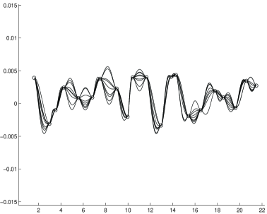
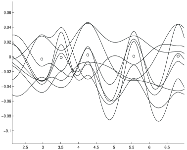
Spline and its derivative are continuous both. In general, for arbitrary coefficients $c_{i}$ we obtain smooth splines with discontinuous second derivative . The examples of such splines are presented on Fig. 2

Figure 2: Examples of smooth polynomial splines of the 4-th order solving the problem B. The choice rule for the coefficients : $c_{i}=\xi$, where $\xi$ is a random value uniformly distributed in the interval $\left[-0.05,0.05\right]$. Points $\left(x_{i},z_{i}\right)$ are marked on the graphs by circles.

If we do not fix parameters $z_{i}$ in (7) then splines solve only the problem A (see Fig . 3)

Figure 3: Examples of polynomial splines of the fourth order from  $C^{2}\left[a,b\right]$ solving the problem A.

$C^{2}$-spline

Let us now construct a spline with the continuous second derivative. For realization of it we must require

$$s_{i-1}^{\prime\prime}\left(x_{i-1}\right)=s_{i}^{\prime\prime}\left(x_{i-1}\right),\ i=\overline{1,N},$$

that tends to the equations

$$c_{i-1}=c_{i}+d_{i}\Delta x_{i}+\frac{e_{i}}{2}\Delta x_{i}^{2}=c_{i}-12\Delta z_{i}\Delta x_{i}^{-2}.$$

This provides the recurrence

$$c_{i}=c_{i-1}+12\Delta z_{i}\Delta x_{i}^{-2},$$ (8)

so

$$c_{i}=c_{0}+12{\displaystyle\sum\limits_{j=1}^{i}}\Delta z_{j}\Delta x_{j}^{-2},\ i=\overline{1,N}.$$

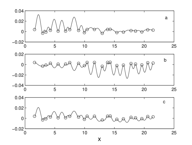
Hence we obtain a one-parameter aggregate of splines of the class $C^{2}\left[a,b\right]$. The parameter of it is $c_{0}$, the second derivative of the spline at the initial point $a$. By choosing of $c_{0}$, we can construct splines with different properties. For example, when

$$c_{0}=-12\min_{i}{\displaystyle\sum\limits_{j=1}^{i}}\Delta z_{j}\Delta x_{j}^{-2},$$

all points of $\mathfrak{M}$ are points of local minima (see Fig. 4, a), for

$$c_{0}=-12\max_{i}{\displaystyle\sum\limits_{j=1}^{i}}\Delta z_{j}\Delta x_{j}^{-2},$$

all points $\mathfrak{M}$ are points of local maxima (see Fig. 4, b), and for

$$c_{0}=-\frac{12}{n}{\displaystyle\sum\limits_{j=1}^{i}}\Delta z_{j}\Delta x_{j}^{-2}.$$

the mean value of the second derivative for over all points of $\mathfrak{M}$ takes its minimum (see Fig. 4, c)

Figure 4: Polynomial splines of the forth order with additional properties: a) all points of $\mathfrak{M}$ are points of local minima, b) all points of $\mathfrak{M}$ are points of local maxima, c) the mean value of the second derivative for over all points of $\mathfrak{M}$ takes its minimum.

3.1.2 Two-dimensional problem ($n=2$)

Consider the following two-dimensional problem B: for given set of points $\left(x_{k},y_{l},z_{kl}\right)$, $a=x_{0}<x_{1}<\ldots<x_{K}=b$, $c=y_{0}<y_{1}<\ldots<y_{L}=d$ build a spline of the 4-th order $F\left(\cdot\right)\in C^{1}\left(\left[a,b\right]\times\left[c,d\right]\right)$ such that

$$\left\{\begin{array}[c]{l}F\left(x,y\right)=s_{kl}\left(x,y\right),\ \left(x,y\right)\in\mathbf{P}_{kl}\equiv\left[x_{k-1},x_{k}\right]\times\left[y_{l-1},y_{l}\right]\ k=\overline{1,K},~{}l=\overline{1,L},\\ s_{kl}\left(x,y\right)={\displaystyle\sum\limits_{i,j=0}^{4}}a_{ij}^{\left(kl\right)}\left(x-x_{k}\right)^{i}\left(y-y_{l}\right)^{j},\\ F\left(x_{k},y_{l}\right)=z_{kl},\\ \triangledown F\left(x_{k},y_{l}\right)=0.\end{array}\right.$$ (9)

By decomposition of the function into one-dimensional splines (6) onto grid lines $\left(x_{k},y_{l}\right),k=\overline{1,K},~{}l=\overline{1,L}$, we receive the following equations for the coefficients of the two-dimensional spline,

$$\begin{array}[c]{ll}{\displaystyle\sum\limits_{i=0}^{4}}\left({\displaystyle\sum\limits_{j=0}^{4}}a_{ij}^{\left(kl\right)}\Delta y_{l}^{j}\right)\left(x-x_{k}\right)^{i}={\displaystyle\sum\limits_{i=0}^{4}}\gamma_{i}^{\left(k\ l-1\right)}\left(x-x_{k}\right)^{i},&y=y_{l-1},\\ {\displaystyle\sum\limits_{i=0}^{4}}a_{i0}^{\left(kl\right)}\left(x-x_{k}\right)^{i}={\displaystyle\sum\limits_{i=0}^{4}}\gamma_{i}^{\left(kl\right)}\left(x-x_{k}\right)^{i},&y=y_{l},\\ {\displaystyle\sum\limits_{j=0}^{4}}\left({\displaystyle\sum\limits_{i=0}^{4}}a_{ij}^{\left(kl\right)}\Delta x_{k}^{i}\right)\left(y-y_{l}\right)^{j}={\displaystyle\sum\limits_{j=0}^{4}}\beta_{j}^{\left(k-1\ l\right)}\left(y-y_{l}\right)^{j},&x=x_{k-1},\\ {\displaystyle\sum\limits_{j=0}^{4}}a_{0j}^{\left(kl\right)}\left(y-y_{l}\right)^{j}={\displaystyle\sum\limits_{j=0}^{4}}\beta_{j}^{\left(kl\right)}\left(y-y_{l}\right)^{j},&x=x_{k},\end{array}$$ (10)

where we know values $\gamma_{i}^{\left(kl\right)},\beta_{j}^{\left(kl\right)}$ from formulae (7); so we know the first column and the first row of the matrix $A^{\left(kl\right)}\equiv\left\{a_{ij}^{\left(kl\right)}\right\}_{i,j=0}^{4}$ . Last $16$ coefficients

$$A^{\left(kl\right)}=\left\|\begin{array}[c]{ccccc}z_{kl}&0&\beta_{2}^{\left(kl\right)}&\beta_{3}^{\left(kl\right)}&\beta_{4}^{\left(kl\right)}\\ 0&a_{11}^{\left(kl\right)}&a_{12}^{\left(kl\right)}&a_{13}^{\left(kl\right)}&a_{14}^{\left(kl\right)}\\ \gamma_{2}^{\left(kl\right)}&a_{21}^{\left(kl\right)}&a_{22}^{\left(kl\right)}&a_{23}^{\left(kl\right)}&a_{24}^{\left(kl\right)}\\ \gamma_{3}^{\left(kl\right)}&a_{31}^{\left(kl\right)}&a_{32}^{\left(kl\right)}&a_{33}^{\left(kl\right)}&a_{34}^{\left(kl\right)}\\ \gamma_{4}^{\left(kl\right)}&a_{41}^{\left(kl\right)}&a_{42}^{\left(kl\right)}&a_{43}^{\left(kl\right)}&a_{44}^{\left(kl\right)}\end{array}\right\|$$

are unknown. For them we have from (10) the equations

$$\left\{\begin{array}[c]{c}{\displaystyle\sum\limits_{j=1}^{4}}a_{ij}^{\left(kl\right)}\Delta y_{l}^{j}=\gamma_{i}^{\left(k\ l-1\right)}-\gamma_{i}^{\left(kl\right)}\equiv\Delta\gamma_{i}^{\left(kl\right)},\ i=\overline{1,4},\\ {\displaystyle\sum\limits_{i=1}^{4}}a_{ij}^{\left(kl\right)}\Delta x_{k}^{i}=\beta_{j}^{\left(k-1\ l\right)}-\beta_{j}^{\left(kl\right)}\equiv\Delta\beta_{j}^{\left(kl\right)},\ j=\overline{1,4}.\end{array}\right.$$ (11)

The matrix of this system is

$$D=\left\|\begin{array}[c]{cccccccc}\Delta y_{l}&0&0&0&\Delta x_{k}&0&0&0\\ \Delta y_{l}^{2}&0&0&0&0&\Delta x_{k}&0&0\\ \Delta y^{3}&0&0&0&0&0&\Delta x_{k}&0\\ \Delta y_{l}^{4}&0&0&0&0&0&0&\Delta x_{k}\\ 0&\Delta y_{l}&0&0&\Delta x_{k}^{2}&0&0&0\\ 0&\Delta y_{l}^{2}&0&0&0&\Delta x_{k}^{2}&0&0\\ 0&\Delta y_{l}^{3}&0&0&0&0&\Delta x_{k}^{2}&0\\ 0&\Delta y_{l}^{4}&0&0&0&0&0&\Delta x_{k}^{2}\\ 0&0&\Delta y_{l}&0&\Delta x_{k}^{3}&0&0&0\\ 0&0&\Delta y_{l}^{2}&0&0&\Delta x_{k}^{3}&0&0\\ 0&0&\Delta y_{l}^{3}&0&0&0&\Delta x_{k}^{3}&0\\ 0&0&\Delta y_{l}^{4}&0&0&0&0&\Delta x_{k}^{3}\\ 0&0&0&\Delta y_{l}&\Delta x_{k}^{4}&0&0&0\\ 0&0&0&y^{2}&0&x^{4}&0&0\\ 0&0&0&y^{3}&0&0&x^{4}&0\\ 0&0&0&y^{4}&0&0&0&x^{4}\end{array}\right\|,$$

and its rank is equal $7$. If we choose

$$a_{11}^{\left(kl\right)},a_{12}^{\left(kl\right)},a_{13}^{\left(kl\right)},a_{14}^{\left(kl\right)},a_{21}^{\left(kl\right)},a_{31}^{\left(kl\right)},a_{41}^{\left(kl\right)},$$

as known values (they correspond to nonzero minor of the order $7$) and choose other $9$ elements as free, then we obtain from (11) the system

$$\left\{\begin{array}[c]{l}a_{11}^{\left(kl\right)}\Delta y_{l}+a_{12}^{\left(kl\right)}\Delta y_{l}^{2}+a_{13}^{\left(kl\right)}\Delta y_{l}^{3}+a_{14}^{\left(kl\right)}\Delta y_{l}^{4}=\Delta\gamma_{1}^{\left(kl\right)}=0,\\ a_{21}^{\left(kl\right)}\Delta y_{l}=\Delta\gamma_{2}^{\left(kl\right)}-a_{22}^{\left(kl\right)}\Delta y_{l}^{2}+a_{23}^{\left(kl\right)}\Delta y_{l}^{3}+a_{24}^{\left(kl\right)}\Delta y_{l}^{4},\\ a_{31}^{\left(kl\right)}\Delta y_{l}=\Delta\gamma_{3}^{\left(kl\right)}-a_{32}^{\left(kl\right)}\Delta y_{l}^{2}+a_{33}^{\left(kl\right)}\Delta y_{l}^{3}+a_{34}^{\left(kl\right)}\Delta y_{l}^{4},\\ a_{41}^{\left(kl\right)}\Delta y_{l}=\Delta\gamma_{4}^{\left(kl\right)}-a_{42}^{\left(kl\right)}\Delta y_{l}^{2}+a_{43}^{\left(kl\right)}\Delta y_{l}^{3}+a_{44}^{\left(kl\right)}\Delta y_{l}^{4},\\ a_{11}^{\left(kl\right)}\Delta x_{k}+a_{21}^{\left(kl\right)}\Delta x_{k}^{2}+a_{31}^{\left(kl\right)}\Delta x_{k}^{3}+a_{41}^{\left(kl\right)}\Delta x_{k}^{4}=\Delta\beta_{1}^{\left(kl\right)}=0,\\ a_{12}^{\left(kl\right)}\Delta x_{k}=\Delta\beta_{2}^{\left(kl\right)}-a_{22}^{\left(kl\right)}\Delta x_{k}^{2}-a_{32}^{\left(kl\right)}\Delta x_{k}^{3}-a_{42}^{\left(kl\right)}\Delta x_{k}^{4},\\ a_{13}^{\left(kl\right)}\Delta x_{k}=\Delta\beta_{3}^{\left(kl\right)}-a_{23}^{\left(kl\right)}\Delta x_{k}^{2}-a_{33}^{\left(kl\right)}\Delta x_{k}^{3}-a_{43}^{\left(kl\right)}\Delta x_{k}^{4}\end{array}\right.$$ (12)

with the solution

$$\left\{\begin{array}[c]{l}a_{13}^{\left(kl\right)}=\Delta\beta_{3}^{\left(kl\right)}\Delta x_{k}^{-1}-a_{23}^{\left(kl\right)}\Delta x_{k}-a_{33}^{\left(kl\right)}\Delta x_{k}^{2}-a_{43}^{\left(kl\right)}\Delta x_{k}^{3},\\ a_{12}^{\left(kl\right)}=\Delta\beta_{2}^{\left(kl\right)}\Delta x_{k}^{-1}-a_{22}^{\left(kl\right)}\Delta x_{k}-a_{32}^{\left(kl\right)}\Delta x_{k}^{2}-a_{42}^{\left(kl\right)}\Delta x_{k}^{3},\\ a_{41}^{\left(kl\right)}=\Delta\gamma_{4}^{\left(kl\right)}\Delta y_{l}^{-1}-a_{42}^{\left(kl\right)}\Delta y_{l}-a_{43}^{\left(kl\right)}\Delta y_{l}^{2}-a_{44}^{\left(kl\right)}\Delta y_{l}^{3},\\ a_{31}^{\left(kl\right)}=\Delta\gamma_{3}^{\left(kl\right)}\Delta y_{l}^{-1}-a_{32}^{\left(kl\right)}\Delta y_{l}-a_{33}^{\left(kl\right)}\Delta y_{l}^{2}-a_{34}^{\left(kl\right)}\Delta y_{l}^{3},\\ a_{21}^{\left(kl\right)}=\Delta\gamma_{2}^{\left(kl\right)}\Delta y_{l}^{-1}-a_{22}^{\left(kl\right)}\Delta y_{l}-a_{23}^{\left(kl\right)}\Delta y_{l}^{2}-a_{24}^{\left(kl\right)}\Delta y_{l}^{3},\\ a_{11}^{\left(kl\right)}=-a_{21}^{\left(kl\right)}\Delta x_{k}-a_{31}^{\left(kl\right)}\Delta x_{k}^{2}-a_{41}^{\left(kl\right)}\Delta x_{k}^{3},\\ a_{14}^{\left(kl\right)}=-a_{11}^{\left(kl\right)}\Delta y_{l}^{-3}-a_{12}^{\left(kl\right)}\Delta y_{l}^{-2}-a_{13}^{\left(kl\right)}\Delta y_{l}^{-1}.\end{array}\right.$$ (13)

$C^{0}$-spline

Let us set, for example, in (13)

$$a_{ij}^{\left(kl\right)}=0,i=\overline{2,4},j=\overline{2,4}.$$

Then we obtain from (13)

$$\left\{\begin{array}[c]{l}a_{13}^{\left(kl\right)}=\Delta\beta_{3}^{\left(kl\right)}\Delta x_{k},\\ a_{12}^{\left(kl\right)}=\Delta\beta_{2}^{\left(kl\right)}\Delta x_{k},\\ a_{41}^{\left(kl\right)}=\Delta\gamma_{4}^{\left(kl\right)}\Delta y_{l},\\ a_{31}^{\left(kl\right)}=\Delta\gamma_{3}^{\left(kl\right)}\Delta y_{l},\\ a_{21}^{\left(kl\right)}=\Delta\gamma_{2}^{\left(kl\right)}\Delta y_{l},\\ a_{11}^{\left(kl\right)}=-\left(\Delta\gamma_{2}^{\left(kl\right)}+\Delta\gamma_{3}^{\left(kl\right)}\Delta x_{k}+\Delta\gamma_{4}^{\left(kl\right)}\Delta x_{k}^{2}\right)\Delta x_{k}\Delta y_{l},\\ a_{14}^{\left(kl\right)}=-a_{11}^{\left(kl\right)}\Delta y_{l}^{-3}-\Delta\beta_{2}^{\left(kl\right)}\Delta x_{k}^{-1}\Delta y_{l}^{-2}-\Delta\beta_{3}^{\left(kl\right)}\Delta x_{k}^{-1}\Delta y_{l}^{-1}.\end{array}\right.$$ (14)

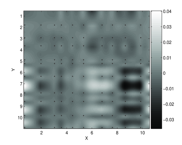
The spline with such coefficients is continuous but, in general, its first derivatives have jumps on the boundaries of the cells $\mathbf{P}_{kl}$. The example of such spline see on Fig. 5

Figure 5: The example of polynomial $C^{0}$-spline with the coefficients (14). The points of $\mathfrak{M}$ are marked by stars, $K=L=10$.

$C^{1}$-spline

Let us try to choose such free parameters that spline (9) becomes $C^{1}$-function. It is sufficiently to require that the first derivative $\partial F/\partial x$ is continuous at all vertical lines $x=x_{k}$ and the $\partial F/\partial y$ is continuous at horizontal lines $y=y_{l}$ of the grid. This tends to the equations

$$\begin{array}[c]{c}a_{1j}^{\left(kl\right)}={\displaystyle\sum\limits_{i=1}^{4}}ia_{ij}^{\left(k+1\ l\right)}\Delta x_{k+1}^{i-1},\ a_{i1}^{\left(kl\right)}={\displaystyle\sum\limits_{j=1}^{4}}ja_{ij}^{\left(k\ l+1\right)}\Delta y_{l+1}^{j-1},\\ j=\overline{1,4},\ i=\overline{2,4},k=\overline{1,K-1},~{}l=\overline{1,L-1}.\end{array}$$ (15)

We see that the second row and the second column of the matrix are completely determined by the coefficients of the matrix from contiguous cells (that lie to right and above from a given cell). On the other hand due to the continuity of the spline and the equations (13) these elements can be found by nine coefficients of the matrix

$$\left\|\begin{array}[c]{ccc}a_{22}^{\left(kl\right)}&a_{23}^{\left(kl\right)}&a_{24}^{\left(kl\right)}\\ a_{32}^{\left(kl\right)}&a_{33}^{\left(kl\right)}&a_{34}^{\left(kl\right)}\\ a_{42}^{\left(kl\right)}&a_{43}^{\left(kl\right)}&a_{44}^{\left(kl\right)}\end{array}\right\|$$ (16)

From the first and the fifth equations of the (12) and from the (15) we receive

$$\begin{array}[c]{c}{\displaystyle\sum\limits_{j=1}^{4}}a_{1j}^{\left(kl\right)}\Delta y_{l}^{j-1}={\displaystyle\sum\limits_{j=1}^{4}}{\displaystyle\sum\limits_{i=1}^{4}}ia_{ij}^{\left(k+1\ l\right)}\Delta x_{k+1}^{i-1}\Delta y_{l}^{j-1}=0,\\ {\displaystyle\sum\limits_{i=1}^{4}}a_{i1}^{\left(kl\right)}\Delta x_{k}^{i-1}={\displaystyle\sum\limits_{i=1}^{4}}{\displaystyle\sum\limits_{j=1}^{4}}ja_{ij}^{\left(k\ l+1\right)}\Delta y_{l+1}^{j-1}\Delta x_{k}^{i-1}=0.\end{array}$$

So we obtain for $a_{ij}^{\left(kl\right)}$

$$\left\{\begin{array}[c]{l}{\displaystyle\sum\limits_{i=1}^{4}}{\displaystyle\sum\limits_{j=1}^{4}}ja_{ij}^{\left(kl\right)}\Delta y_{l}^{j-1}\Delta x_{k}^{i-1}=0,\\ {\displaystyle\sum\limits_{j=1}^{4}}{\displaystyle\sum\limits_{i=1}^{4}}ia_{ij}^{\left(kl\right)}\Delta x_{k}^{i-1}\Delta y_{l}^{j-1}=0.\end{array}\right.$$ (17)

Five additional equations we obtain from the system (12),

$$\left\{\begin{array}[c]{l}a_{22}^{\left(kl\right)}+a_{32}^{\left(kl\right)}\Delta x_{k}+a_{42}^{\left(kl\right)}\Delta x_{k}^{2}=\Delta\beta_{2}^{\left(kl\right)}\Delta x_{k}^{-2}-a_{12}^{\left(kl\right)}\Delta x_{k}^{-1},\\ a_{23}^{\left(kl\right)}+a_{33}^{\left(kl\right)}\Delta x_{k}+a_{43}^{\left(kl\right)}\Delta x_{k}^{2}=\Delta\beta_{3}^{\left(kl\right)}\Delta x_{k}^{-2}-a_{13}^{\left(kl\right)}\Delta x_{k}^{-1},\\ a_{22}^{\left(kl\right)}+a_{23}^{\left(kl\right)}\Delta y_{l}+a_{24}^{\left(kl\right)}\Delta y_{l}^{2}=\Delta\gamma_{2}^{\left(kl\right)}\Delta y_{l}^{-2}-a_{21}^{\left(kl\right)}\Delta y_{l}^{-1},\\ a_{32}^{\left(kl\right)}+a_{33}^{\left(kl\right)}\Delta y_{l}+a_{34}^{\left(kl\right)}\Delta y_{l}^{2}=\Delta\gamma_{3}^{\left(kl\right)}\Delta y_{l}^{-2}-a_{31}^{\left(kl\right)}\Delta y_{l}^{-1},\\ a_{42}^{\left(kl\right)}+a_{43}^{\left(kl\right)}\Delta y_{l}+a_{44}^{\left(kl\right)}\Delta y_{l}^{2}=\Delta\gamma_{4}^{\left(kl\right)}\Delta y_{l}^{-2}-a_{41}^{\left(kl\right)}\Delta y_{l}^{-1}.\end{array}\right.$$ (18)

From systems (18) and (17) we receive the system of seven equations for nine coefficients (16)

$$\left\{\begin{array}[c]{l}a_{22}^{\left(kl\right)}+a_{32}^{\left(kl\right)}\Delta x_{k}+a_{42}^{\left(kl\right)}\Delta x_{k}^{2}=\Delta\beta_{2}^{\left(kl\right)}\Delta x_{k}^{-2}-a_{12}^{\left(kl\right)}\Delta x_{k}^{-1},\\ a_{23}^{\left(kl\right)}+a_{33}^{\left(kl\right)}\Delta x_{k}+a_{43}^{\left(kl\right)}\Delta x_{k}^{2}=\Delta\beta_{3}^{\left(kl\right)}\Delta x_{k}^{-2}-a_{13}^{\left(kl\right)}\Delta x_{k}^{-1},\\ a_{22}^{\left(kl\right)}+a_{23}^{\left(kl\right)}\Delta y_{l}+a_{24}^{\left(kl\right)}\Delta y_{l}^{2}=\Delta\gamma_{2}^{\left(kl\right)}\Delta y_{l}^{-2}-a_{21}^{\left(kl\right)}\Delta y_{l}^{-1},\\ a_{32}^{\left(kl\right)}+a_{33}^{\left(kl\right)}\Delta y_{l}+a_{34}^{\left(kl\right)}\Delta y_{l}^{2}=\Delta\gamma_{3}^{\left(kl\right)}\Delta y_{l}^{-2}-a_{31}^{\left(kl\right)}\Delta y_{l}^{-1},\\ a_{42}^{\left(kl\right)}+a_{43}^{\left(kl\right)}\Delta y_{l}+a_{44}^{\left(kl\right)}\Delta y_{l}^{2}=\Delta\gamma_{4}^{\left(kl\right)}\Delta y_{l}^{-2}-a_{41}^{\left(kl\right)}\Delta y_{l}^{-1},\\ {\displaystyle\sum\limits_{i=2}^{4}}{\displaystyle\sum\limits_{j=2}^{4}}ja_{ij}^{\left(kl\right)}\Delta y_{l}^{j-1}\Delta x_{k}^{i-1}=-{\displaystyle\sum\limits_{j=1}^{4}}ja_{1j}^{\left(kl\right)}\Delta y_{l}^{j-1}-{\displaystyle\sum\limits_{i=2}^{4}}a_{i1}^{\left(kl\right)}\Delta x_{k}^{i-1},\\ {\displaystyle\sum\limits_{j=2}^{4}}{\displaystyle\sum\limits_{i=2}^{4}}ia_{ij}^{\left(kl\right)}\Delta y_{l}^{j-1}\Delta x_{k}^{i-1}=-{\displaystyle\sum\limits_{j=1}^{4}}a_{1j}^{\left(kl\right)}\Delta y_{l}^{j-1}-{\displaystyle\sum\limits_{i=2}^{4}}ia_{i1}^{\left(kl\right)}\Delta x_{k}^{i-1}.\end{array}\right.$$ (19)

However the matrix of this system

$$\left\|\begin{array}[c]{ccccccc}1&0&1&0&0&2\Delta y_{l}\Delta x_{k}&2\Delta x_{k}\Delta y_{l}\\ \Delta x_{k}&0&0&1&0&2\Delta y_{l}\Delta x_{k}^{2}&3\Delta x_{k}^{2}\Delta y_{l}\\ \Delta x_{k}^{2}&0&0&0&1&2\Delta y_{l}\Delta x_{k}^{3}&4\Delta x_{k}^{3}\Delta y_{l}\\ 0&1&\Delta y_{l}&0&0&3\Delta y_{l}^{2}\Delta x_{k}&2\Delta x_{k}\Delta y_{l}^{2}\\ 0&\Delta x_{k}&0&\Delta y_{l}&0&3\Delta y_{l}^{2}\Delta x_{k}^{2}&3\Delta x_{k}^{2}\Delta y_{l}^{2}\\ 0&\Delta x_{k}^{2}&0&0&\Delta y_{l}&3\Delta y_{l}^{2}\Delta x_{k}^{3}&4\Delta x_{k}^{3}\Delta y_{l}^{2}\\ 0&0&\Delta y_{l}^{2}&0&0&4\Delta y_{l}^{3}\Delta x_{k}&2\Delta x_{k}\Delta y_{l}^{3}\\ 0&0&0&\Delta y_{l}^{2}&0&4\Delta y_{l}^{3}\Delta x_{k}^{2}&3\Delta x_{k}^{2}\Delta y_{l}^{3}\\ 0&0&0&0&\Delta y_{l}^{2}&4\Delta y_{l}^{3}\Delta x_{k}^{3}&4\Delta x_{k}^{3}\Delta y_{l}^{3}\end{array}\right\|$$

has the rank $5$. This means that system (19) has no solution. Hence two-dimensional problem B has no solution in the class of $C^{1}$-splines.

Besides the problem of smoothness the next problem is the appearance of false stationary points that do not belong to $\mathfrak{M}$. The above considerations show that class of polynomial splines is not convenient for solutions of the problem B,C.

3.2 Trigonometric splines

3.2.1 One-dimensional problem

Consider the following problem B: for given sets $\left(x_{i},z_{i}\right)$, $a=x_{0}<x_{1}<\ldots<x_{N}=b$ build a trigonometric spline $F\left(\cdot\right)\in C^{1}\left[a,b\right]$ such that

$$\left\{\begin{array}[c]{l}F\left(x\right)=t_{i}\left(x\right),\ x\in\left[x_{i-1},x_{i}\right],\ i=\overline{1,N},\\ t_{i}\left(x\right)\equiv a_{i}+b_{i}\cos\left(c_{i}x+d_{i}\right),\\ F\left(x_{i}\right)=z_{i},\\ F^{\prime}\left(x_{i}\right)=0.\end{array}\right.$$ (20)

Conditions (20) do not identify the spline. For example, we can take the following coefficients

$$\left\{\begin{array}[c]{l}a_{i}=\left(z_{i-1}+z_{i}\right)/2,\\ b_{i}=\left(z_{i-1}-z_{i}\right)/2,\\ c_{i}=\pi/\bigtriangleup x_{i},\\ d_{i}=-\pi x_{i-1}/\bigtriangleup x_{i},\\ \bigtriangleup x_{i}\equiv x_{i}-x_{i-1}.\end{array}\right.$$

The corresponding spline has the form

$$t_{i}\left(x\right)=\frac{z_{i-1}+z_{i}}{2}+\frac{z_{i-1}-z_{i}}{2}\cos\pi\frac{x-x_{i-1}}{\bigtriangleup x_{i}}.$$

For such coefficients false stationary points are absent; this means that really the spline solves the problem C.

In general, for arbitrary values $z_{i}$ the spline has jumps at points $x_{i}$. If to forbid the jumps,

$$\begin{array}[c]{c}t_{i-1}^{\prime\prime}\left(x_{i-1}+0\right)=-\pi^{2}\left(z_{i-2}-z_{i-1}\right)\bigtriangleup x_{i-1}^{-2}/2=\\ =\pi^{2}\left(z_{i-1}-z_{i}\right)\bigtriangleup x_{i}^{-2}/2=t_{i}^{\prime\prime}\left(x_{i-1}-0\right),\end{array}$$

then we receive the relations

$$\left(z_{i}-z_{i-1}\right)/\bigtriangleup x_{i}^{2}=\mu\left(-1\right)^{i},\ i=\overline{1,n},$$

where $\mu$ is an arbitrary value. Such kind ²-splines form two-parametrical set as for fixed value $z_{0}$ other values $z_{i}$ can be calculated by the formula

$$z_{i}=z_{0}+\mu{\displaystyle\sum\limits_{l=1}^{i}}\left(-1\right)^{l}\bigtriangleup x_{l}^{2}$$ (21)

which contains two free parameters $z_{0}$ and $\mu.$ For fixed set $\left\{x_{i}\right\}$ the parameter $\mu$ evaluates mean deviation of the spline from the initial value $z_{0}$:

$${\displaystyle\sum\limits_{i=1}^{n}}\left(z_{i}-z_{0}\right)/n=\mu{\displaystyle\sum\limits_{l=1}^{n}}\left(-1\right)^{l}\left(1-l/n\right)\bigtriangleup x_{l}^{2}.$$

Examples of trigonometric splines (20) are presented on Fig. 6

Figure 6: A beam of smooth trigonometric splines. The values $\left\{z_{i}\right\}$ were taken randomly from a given interval.

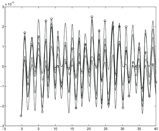
3.2.2 Two-dimensional problem

Consider the following problem B: for given sets $\left(x_{k},y_{l},z_{kl}\right)$, $a=x_{0}<x_{1}<\ldots<x_{K}=b$, $c=y_{0}<y_{1}<\ldots<y_{L}=d$ build a spline $F\left(\cdot\right)\in C^{1}\left(\left[a,b\right]\times\left[c,d\right]\right)$ such that

$$\left\{\begin{array}[c]{l}F\left(x,y\right)=t_{kl}\left(x,y\right),\ \left(x,y\right)\in\mathbf{P}_{kl},\ k=\overline{1,K},~{}l=\overline{1,L},\\ t_{kl}\left(x,y\right)=\left[a_{kl}+b_{kl}\cos\left(c_{kl}x+d_{kl}\right)\right]\left[A_{kl}+B_{kl}\cos\left(C_{kl}y+D_{kl}\right)\right],\\ F\left(x_{k},y_{l}\right)=z_{kl},\\ \triangledown F\left(x_{k},y_{l}\right)=0.\end{array}\right.$$ (22)

In analogues to one-dimensional case the conditions (22) do not identify the spline. For example, we can take

$$\left\{\begin{array}[c]{l}c_{kl}=\pi/\Delta x_{k},\\ d_{kl}=-\pi x_{k-1}/\Delta x_{k},\\ C_{kl}=\pi/\Delta y_{l},\\ D_{kl}=-\pi y_{l-1}/\Delta y_{l},\end{array}\right.$$ (23)

where $\Delta x_{k}\equiv x_{k}-x_{k-1}$, $\Delta y_{l}\equiv y_{l}-y_{l-1}$. In this case $\triangledown F\left(x_{k},y_{l}\right)=0$ at the vertex of $\mathbf{P}_{kl}$ (and only at these points; so, actually the spline solves the problem C). For other coefficients of the spline we have the equations

$$\left\{\begin{array}[c]{l}t_{kl}\left(x_{k-1},y_{l-1}\right)=\left[a_{kl}+b_{kl}\right]\left[A_{kl}+B_{kl}\right]=z_{k-1l-1},\\ t_{kl}\left(x_{k},y_{l-1}\right)=\left[a_{kl}-b_{kl}\right]\left[A_{kl}+B_{kl}\right]=z_{kl-1},\\ t_{kl}\left(x_{k-1},y_{l}\right)=\left[a_{kl}+b_{kl}\right]\left[A_{kl}-B_{kl}\right]=z_{k-1l},\\ t_{kl}\left(x_{k},y_{l}\right)=\left[a_{kl}-b_{kl}\right]\left[A_{kl}-B_{kl}\right]=z_{kl}\end{array}\right.$$

which give

$$\left\{\begin{array}[c]{l}a_{kl}A_{kl}=\left(z_{k-1l-1}+z_{k-1l}+z_{kl-1}+z_{kl}\right)/4,\\ b_{kl}A_{kl}=\left(z_{k-1l-1}+z_{k-1l}-z_{kl-1}-z_{kl}\right)/4,\\ a_{kl}B_{kl}=\left(z_{k-1l-1}+z_{kl-1}-z_{k-1l}-z_{kl}\right)/4,\\ b_{kl}B_{kl}=\left(z_{k-1l-1}+z_{kl}-z_{k-1l}-z_{kl-1}\right)/4,\end{array}\right.$$ (24)

that is sufficient for the spline determination. As coefficients of $t_{kl}\left(x,y\right)$ depend only on the spline values at vertexes of $\mathbf{P}_{kl}$, then we must restrict these values in order to provide the smoothness of the spline.

It is easy to prove that we need to provide the smoothness of the spline on the boundaries of $\mathbf{P}_{kl}$ only. Take for example the common boundary of $\mathbf{P}_{kl}$ and $\mathbf{P}_{kl-1}$, the segment $\left[x_{k-1},x_{k}\right]\times\left\{y_{l-1}\right\}$. The spline is continuous on this segment if and only if for all $x\in\left[x_{k-1},x_{k}\right]$

$$\begin{array}[c]{c}\left[a_{kl}+b_{kl}\cos\pi\left(x-x_{k-1}\right)/\Delta x_{k}\right]\left[A_{kl}+B_{kl}\right]=\\ =\left[a_{kl-1}+b_{kl-1}\cos\pi\left(x-x_{k-1}\right)/\Delta x_{k}\right]\left[A_{kl-1}-B_{kl-1}\right].\end{array}$$

So we have the equations

$$\left\{\begin{array}[c]{l}a_{kl-1}\left(A_{kl-1}-B_{kl-1}\right)=a_{kl}\left(A_{kl}+B_{kl}\right),\\ b_{kl-1}\left(A_{kl-1}-B_{kl-1}\right)=b_{kl}\left(A_{kl}+B_{kl}\right).\end{array}\right.$$ (25)

Substitute formulae (24) to these equations we receive the identities for $z_{kl}$. Also we get the identities when check the continuity of the spline on the vertical boundary $\left\{x_{k-1}\right\}\times\left[y_{l-1},y_{l}\right]$. Hence the spline is continuous for all values $\left\{z_{kl}\right\}$. Actually the spline belongs even to the class $C^{1}\left(\left[a,b\right]\times\left[c,d\right]\right)$. To prove it we must prove the continuity of the gradient on the boundaries of $\mathbf{P}_{kl}$. For example, using (25), we have on the segment $\left[x_{k-1},x_{k}\right]\times\left\{y_{l-1}\right\}$

$$\begin{array}[c]{l}F_{y}^{\prime}\left(x,y_{l-1}\pm 0\right)\equiv 0,\\ F_{x}^{\prime}\left(x,y_{l-1}\pm 0\right)\equiv\pi b_{kl}\sin\left(\pi\left(x-x_{k-1}\right)/\Delta x_{k}\right)\left[A_{kl}+B_{kl}\right]/\Delta x_{k}\equiv\\ \equiv\pi b_{kl-1}\sin\left(\pi\left(x-x_{k-1}\right)/\Delta x_{k}\right)\left[A_{kl-1}-B_{kl-1}\right]/\Delta x_{k}.\end{array}$$

If we want to construct the more smooth spline then we must to impose its values $\left\{z_{kl}\right\}$. For example the condition of continuity of the second derivative $F_{y^{2}}^{\prime\prime}$ on the boundary $\left[x_{k-1},x_{k}\right]\times\left\{y_{l-1}\right\}$ tends to the equations

$$\begin{array}[c]{c}\left[a_{kl}+b_{kl}\cos\pi\left(x-x_{k-1}\right)/\Delta x_{k}\right]B_{kl}C_{kl}^{2}=\\ =-\left[a_{kl-1}+b_{kl-1}\cos\pi\left(x-x_{k-1}\right)/\Delta x_{k}\right]B_{kl-1}C_{kl-1}^{2},\end{array}$$

hence,

$$a_{kl}B_{kl}C_{kl}^{2}=-a_{kl-1}B_{kl-1}C_{kl-1}^{2},\ b_{kl}B_{kl}C_{kl}^{2}=-b_{kl-1}B_{kl-1}C_{kl-1}^{2}.$$

If we put (24) to these equalities, then we get

$$\begin{array}[c]{c}\left(z_{k-1l-1}+z_{kl-1}-z_{k-1l}-z_{kl}\right)\beta_{l}=\left(z_{k-1l-1}+z_{kl-1}-z_{k-1l-2}-z_{kl-2}\right),\\ \left(z_{k-1l-1}+z_{kl}-z_{k-1l}-z_{kl-1}\right)\beta_{l}=\left(z_{k-1l-1}+z_{kl-2}-z_{k-1l-2}-z_{kl-1}\right),\end{array}$$ (26)

where $\beta_{l}\equiv\left(\Delta y_{l-1}/\Delta y_{l}\right)^{2}$. In analogues the condition of continuity of the second derivative $F_{x^{2}}^{\prime\prime}$ on the boundary$\left\{x_{k-1}\right\}\times\left[y_{l-1},y_{l}\right]$ tends to the equations

$$\begin{array}[c]{c}\left[A_{kl}+B_{kl}\cos\pi\left(y-y_{l-1}\right)/\Delta y_{l}\right]b_{kl}c_{kl}^{2}=\\ =-\left[A_{k-1l}+B_{k-1l}\cos\pi\left(y-y_{l-1}\right)/\Delta y_{l}\right]b_{k-1l}c_{k-1l}^{2},\end{array}$$

hence,

$$A_{kl}b_{kl}c_{kl}^{2}=-A_{k-1l}b_{k-1l}c_{k-1l}^{2},\ B_{kl}b_{kl}c_{kl}^{2}=-B_{k-1l}b_{k-1l}c_{k-1l}^{2},$$

and

$$\begin{array}[c]{c}\left(z_{k-1l-1}+z_{k-1l}-z_{kl-1}-z_{kl}\right)\delta_{k}=z_{k-1l-1}+z_{k-1l}-z_{k-2l-1}-z_{k-2l},\\ \left(z_{k-1l-1}+z_{kl}-z_{k-1l}-z_{kl-1}\right)\delta_{k}=z_{k-2l}+z_{k-1l-1}-z_{k-2l-1}-z_{k-1l},\end{array}$$ (27)

where $\delta_{k}\equiv\left(\Delta x_{k-1}/\Delta x_{k}\right)^{2}$. It is easy to prove that other derivatives of the second order are also continuous in this case.

From (26) and (27) we have

$$\left\{\begin{array}[c]{l}z_{kl-2}=\beta_{l}z_{kl}+z_{kl-1}\left(1-\beta_{l}\right),\\ z_{k-1l-2}=\beta_{l}z_{k-1l}+z_{k-1l-1}\left(1-\beta_{l}\right),\\ z_{k-2l}=\delta_{k}z_{kl}+z_{k-1l}\left(1-\delta_{k}\right),\\ z_{k-2l-1}=\delta_{k}z_{kl-1}+z_{k-1l-1}\left(1-\delta_{k}\right).\end{array}\right.$$

Differently these formulas can be written in the form

$$\begin{array}[c]{l}\left(z_{kl-1}-z_{kl-2}\right)/\Delta y_{l-1}^{2}=-\left(z_{kl}-z_{kl-1}\right)/\Delta y_{l}^{2},\\ \left(z_{k-1l}-z_{k-2l}\right)/\Delta x_{k-1}^{2}=-\left(z_{kl}-z_{k-1l}\right)/\Delta x_{k}^{2},\end{array}$$

and this means that

$$\begin{array}[c]{c}\left(z_{kl}-z_{kl-1}\right)/\Delta y_{l}^{2}=\left(-1\right)^{l}\mu_{k},\ l=\overline{1,L},\ k=\overline{0,K}\\ \left(z_{kl}-z_{k-1l}\right)/\Delta x_{k}^{2}=\left(-1\right)^{k}\nu_{l},\ k=\overline{1,K},\ l=\overline{0,L}\end{array}$$

for some sets of values $\left\{\mu_{k}\right\},$ $\left\{\nu_{l}\right\}$. So,

$$z_{kl}=z_{k0}+\mu_{k}{\displaystyle\sum\limits_{j=1}^{l}}\left(-1\right)^{j}\Delta y_{j}^{2}=z_{0l}+\nu_{l}{\displaystyle\sum\limits_{i=1}^{k}}\left(-1\right)^{i}\Delta x_{i}^{2},$$

$$z_{kl}-z_{k-1l}=z_{k0}-z_{k-10}+\left(\mu_{k}-\mu_{k-1}\right){\displaystyle\sum\limits_{j=1}^{l}}\left(-1\right)^{j}\Delta y_{j}^{2}=\nu_{l}\left(-1\right)^{k}\Delta x_{k}^{2},$$

$$\left(-1\right)^{k}\frac{\left(\mu_{k}-\mu_{k-1}\right)}{\Delta x_{k}^{2}}{\displaystyle\sum\limits_{j=1}^{l}}\left(-1\right)^{j}\Delta y_{j}^{2}=\nu_{l}-\nu_{0}.$$

For fulfilment of the last equalities for all $k,l$ one can take for any value $\lambda$

$$\mu_{k}=\mu_{0}+\lambda{\displaystyle\sum\limits_{j=1}^{k}}\left(-1\right)^{j}\Delta x_{j}^{2}.$$

In this case

$$\nu_{l}=\nu_{0}+\lambda{\displaystyle\sum\limits_{j=1}^{l}}\left(-1\right)^{j}\Delta y_{j}^{2},$$

$$\begin{array}[c]{c}z_{kl}=z_{00}+\nu_{0}{\displaystyle\sum\limits_{i=1}^{k}}\left(-1\right)^{i}\Delta x_{i}^{2}+\mu_{0}{\displaystyle\sum\limits_{j=1}^{l}}\left(-1\right)^{j}\Delta y_{j}^{2}+\\ +\lambda{\displaystyle\sum\limits_{i=1}^{k}}\left(-1\right)^{i}\Delta x_{i}^{2}{\displaystyle\sum\limits_{j=1}^{l}}\left(-1\right)^{j}\Delta y_{j}^{2}.\end{array}$$ (28)

We see that this family of ²-splines depends only on the next four free parameters $z_{00},\nu_{0},\mu_{0},\lambda.$

Examples of two-dimensional trigonometric splines see in Figs. 7,8.

Figure 7: An example of two-dimensional trigonometric spline (22). Values $\left\{z_{ij}\right\},$ $i,j=\overline{1,10}$ were taken randomly from a fixed segment.

Figure 8: An example of two-dimensional trigonometric $C^{2}$-spline (22). Values $\left\{z_{ij}\right\},$ $i,j=\overline{1,10}$ were calculated by the formula ( 28).

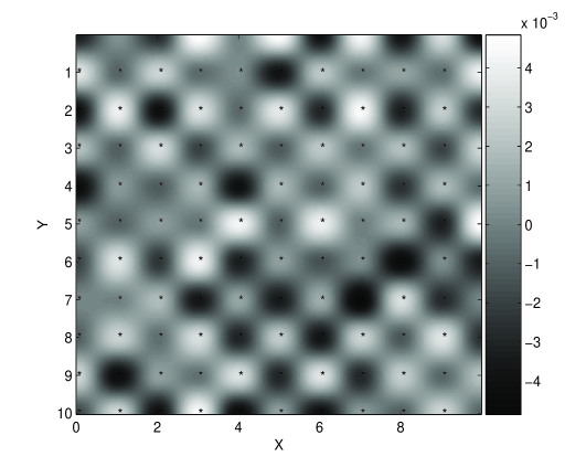
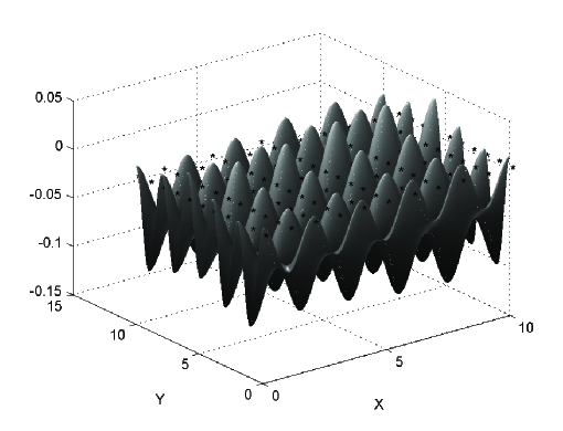
4 Superpositions of splines

In the last section we have established that for two-dimensional sets $\mathfrak{M}$ with matrix structure (5) solutions of the problems A-C can be found in the form of splines (polynomial or trigonometric with different types of smoothness). If $\mathfrak{M}$ does not have the matrix form any spline has an additional (false) points where its gradient equals to zero; so it can not solve the problem C. To overcome this obstacle some constructions may be proposed.

For example, consider the following procedure consisting of the steps

Step 1.

Complete $\mathfrak{M}$ to a set $\mathfrak{M}_{XY}$ of the matrix form and build any spline $F\left(x,y;\mathfrak{M}_{XY}\right)$ that solves the corresponding problem C;

Step 2.

Turn the coordinate system $XY$ for some (”sufficiently small”) angle $\varphi_{1}$ and build an analogous spline in the coordinates $X_{1}Y_{1}$,

$$F\left(x_{{}_{1}},y_{{}_{1}};\mathfrak{M}_{X_{1}Y_{1}}\right)\equiv F\left(x\cos\varphi_{1}-y\sin\varphi_{1},x\sin\varphi_{1}+y\cos\varphi_{1};\mathfrak{M}_{X_{1}Y_{1}}\right);$$

Step 3.

Repeat the above steps several times for different angles $\varphi_{k}$; then build the function

$$\tilde{F}\left(x,y\right)={\displaystyle\sum\limits_{k\geq 1}}F\left(x\cos\varphi_{k}-y\sin\varphi_{k},x\sin\varphi_{k}+y\cos\varphi_{k};\mathfrak{M}_{X_{k}Y_{k}}\right).$$ (29)

As gradients of all summands are zero at points $\mathfrak{M}$, the function $\tilde{F}\left(x,y\right)$ (superposition of splines) solves the problem A. At the same time the additional points for matrixes $\mathfrak{M}_{X_{k}Y_{k}}$ are not the same (they are removed from their initial places); so, the probability that gradients of the summary function (29) at additional points are not zero is high. Test calculations verify these assumption.