Gravitational wave astronomy of single sources with a pulsar timing array

Abstract

The stability of radio millisecond pulsars as celestial clocks allows for the possibility to detect and study the properties of gravitational waves (GWs) when the received pulses are timed jointly in a “Pulsar Timing Array” (PTA) experiment. Here, we investigate the potential of detecting the gravitational wave from individual binary black hole systems using PTAs and calculate the accuracy for determining the GW properties. This is done in a consistent analysis, which at the same time accounts for the measurement of the pulsar distances via the timing parallax.

We find that, at low redshift, a PTA is able to detect the nano-Hertz GW from super massive black hole binary systems with masses of $\sim 10^{8}-10^{10}\,M_{\sun}$ less than $\sim 10^{5}$ years before the final merger. Binaries with more than $\sim 10^{3}-10^{4}$ years before merger are effectively monochromatic GW, and those with less than $\sim 10^{3}-10^{4}$ years before merger may allow us to detect the evolution of binaries.

For our findings, we derive an analytical expression to describe the accuracy of a pulsar distance measurement via timing parallax. We consider five years of bi-weekly observations at a precision of 15 ns for close-by ($\sim 0.5-1$ kpc) pulsars. Timing twenty pulsars would allow us to detect a GW source with an amplitude larger than $5\times 10^{-17}$. We calculate the corresponding GW and binary orbital parameters and their measurement precision. The accuracy of measuring the binary orbital inclination angle, the sky position, and the GW frequency are calculated as functions of the GW amplitude. We note that the “pulsar term”, which is commonly regarded as noise, is essential for obtaining an accurate measurement for the GW source location.

We also show that utilizing the information encoded in the GW signal passing the Earth also increases the accuracy of pulsar distance measurements. If the gravitational wave is strong enough, one can achieve sub-parsec distance measurements for nearby pulsars with distance less than $\sim 0.5-1$ kpc.

1 Introduction

Gravitational waves (GWs), ripples in space-time, perturb our four dimensional space-time background, on which the pulsed radio radiation from pulsars propagates. Through such space-time background perturbations, the GW leaves its fingerprint in the arrival times of pulsar signals by introducing an extra correlated component (Sazhin, 1978; Detweiler, 1979; Bertotti et al., 1983; Wahlquist, 1987; Backer & Hellings, 1986). By timing multiple pulsars (quasi-)simultaneously in a so-called “Pulsar Timing Array” (PTA) experiment, one can extract the GW signal, even in the presence of various unrelated noise contributions in the timing data (Romani & Taylor, 1983; Hellings & Downs, 1983; Blandford et al., 1984; Foster & Backer, 1990; Jenet et al., 2004; Jenet et al., 2005; Sesana & Vecchio, 2010; Finn & Lommen, 2010).

In general, GW sources are classified into two groups, the single sources and a stochastic background component. A stochastic GW background is a superposition of multiple single GW sources, which are inseparable in frequency space (Cutler & Thorne, 2001; Thorne, 1989) due to finite frequency resolution of finite data. The techniques of detecting a single GW source and that of detecting a stochastic background are therefore quite different. The detection of a stochastic GW background using pulsar timing has already been addressed in various studies (Detweiler, 1979; Hellings & Downs, 1983; Backer & Hellings, 1986; Jenet et al., 2005; Hobbs et al., 2009). Here we concentrate on single GW sources.

Recently, many authors have drawn attention to the single source detection problem (Jenet et al., 2004; Sesana & Vecchio, 2010; Burt et al., 2010; Finn & Lommen, 2010; Yardley et al., 2010; Deng & Finn, 2010; Corbin & Cornish, 2010), because of possible nearby ($z\ll 1$) coalescing binary systems that produce GW signals detectable with PTAs (Wen et al., 2009; Sesana et al., 2009; Burke-Spolaor, 2010). In this paper, we focus on the problem of detecting GWs from super-massive black hole binaries (SMBHB), with masses from $10^{8}$ $M_{\sun}$ to $10^{10}$ $M_{\sun}$ and orbital frequencies in the nano-Hertz range, which makes these SMBHBs indeed potential GW sources for PTA projects. We will show how PTAs can be used to measure the parameters of SMBHBs and their GWs.

The plan for the paper is as follows. We begin with a qualitative estimation of the parameter space of the detectable SMBHB population for PTAs in § 2. We then calculate the parameter estimation error for the GW parameters in § 3 where we describe the timing response to a single GW source § 3.1, and present a careful and correct treatment of the corresponding statistical problems § 3.2. Finally, we summarize and discuss our results in § 4.

2 The detectable black hole binary population

In order to use the time-of-arrival (TOA) data from a PTA to detect GWs and infer their parameters, two conditions have to be met. First, the GW amplitude is large enough such that its statistic is significant to confirm the detection, and secondly, the GW frequency is in a frequency window where the pulsar timing technique is sensitive. In this section, we will estimate the parameter space of the GW sources, i.e. the parameter space of super massive black hole binaries (SMBHBs), where they are observable to practical PTAs.

For a PTA, one needs at least five parameters to specify its configuration, i.e. the number of pulsars ($N_{\rm psr}$) in the array, the accuracy of the TOA ($\sigma_{\rm n}$), the total observing time span ($T$), the duration ($\Delta T$) between two successive observing sessions, and the pulsar distances $D_{\rm psr}$. These parameters describe both the amplitude and frequency characteristics of a PTA. For detecting a stochastic GW background, we do not need pulsar distances (Jenet et al., 2005). But as we will explain later, for a single GW source, pulsar distances play an important role and need to be taken into account in the analysis (Jenet et al., 2004; Sesana et al., 2009; Finn & Lommen, 2010).

$T$ and $\Delta T$ determine the frequency characteristics of PTAs. For example, the frequency resolution of a PTA is $\Delta f\approx 1/T$, and the Nyquist frequency, the maximal recoverable frequency is given by $f_{\rm max}\approx 1/(2\Delta T)$. In the standard pulsar timing data reduction pipeline (Backer & Hellings, 1986; Hobbs et al., 2009; Lorimer & Kramer, 2005), one fits for the periods and period derivatives of pulsars. This removes the lowest-frequency components in the pulsar timing data, and the minimal recoverable frequency $f_{\rm min}$ in the pulsar timing data is $f_{\rm min}\approx\Delta f=1/T$ (Jenet et al., 2005). $N_{\rm psr}$ and $\sigma_{\rm n}$ determine the amplitude characteristics of the PTAs. One can detect a coherent sinusoidal signal among all the pulsars in the PTA, if the amplitude of the signal is larger than (Scargle, 1982) $\sigma_{\rm n}/\sqrt{N_{\rm psr}N_{\rm obs}}$, where $N_{\rm obs}$ denotes the average number of independent TOA measurements for each pulsar. The pulsar distance $D_{\rm psr}$ plays two roles in the whole picture. As we will show, it introduces another signal component in the pulsar TOA data, i.e. the “pulsar term”, which increases the signal-to-noise and also gives a very long time baseline to investigate the GW evolution (Jenet et al., 2004).

The mean GW amplitude $\bar{h}$ from a SMBHB averaged over the solid angle of all orbital orientations of the binary, in units where $G=c=1$, is (Thorne, 1989; Wen et al., 2009)

$$\bar{h}\equiv\sqrt{\langle|h_{+}|^{2}+|h_{\times}|^{2}\rangle}=2\left(\frac{32}{125}\right)^{1/6}\frac{{\cal M}^{5/3}\omega_{\rm g}^{2/3}(1+z)^{2/3}}{D_{\rm c}}\;,$$ (1)

where $h_{+}$ and $h_{\times}$ are the ‘plus’ and ‘cross’ gravitational-wave amplitudes, and $\cal M$, $z$ and $D_{\rm c}$ are the chirp mass, the cosmological redshift, and the co-moving distance of the binary. The $\omega_{\rm g}$ is the GW angular frequency at the observer. In the standard cosmology model, the co-moving distance $D_{\rm c}$ is

$$D_{\rm c}=\frac{1}{H_{0}}\int_{0}^{z}\frac{dz}{\sqrt{\Omega_{\Lambda}+\Omega_{\rm M}(1+z)^{3}}}\;.$$ (2)

where we used the dark energy density $\Omega_{\rm\Lambda}=0.7$, matter density $\Omega_{\rm M}=0.3$, and the Hubble constant $H_{0}=73$ ${\rm kms^{-1}\,Mpc^{-1}}=2.37\times 10^{-18}$ ${\rm s^{-1}}$ (Particle Data Group, 2008). The angular frequency relates to the black hole binary chirp mass and the time before final merger of the binary via (Hughes, 2009)

$$\omega_{\rm g}=2\left(\frac{5}{256}\right)^{3/8}\frac{1}{{\cal M}^{5/8}t_{\rm m}^{3/8}(1+z)^{5/8}}\;,$$ (3)

where $t_{\rm m}$ is the time before final coalescence of the binary system at the observer, i.e. the time span between the time of ‘present’ to the time of the binary’s final merger. The GW radiation takes away the energy of the SMBHB, which induces a frequency chirping GW. The angular frequency of the GWs increases at the rate of $\dot{\omega}_{\rm g}$, where

$$\dot{\omega}_{\rm g}=\frac{3}{4}\left(\frac{5}{256}\right)^{3/8}\frac{1}{{\cal M}^{5/8}t_{\rm m}^{11/8}(1+z)^{5/8}}\;.$$ (4)

The GWs from a black hole binary introduce signals in the pulsar TOA data. It turns out that the GW induced timing signal $R(t)$ depends on both the GW strain at the pulsar and the GW strain at the Earth, i.e. $R(t)\sim\left[h(t,0)-h(t-D_{\rm psr},{\rm\bf D_{\rm psr}})\right]/2\omega_{g}$ (Estabrook & Wahlquist, 1975) . The $h(t,0)$, the Earth term, is the GW strain at the Earth at the time when we receive the pulse; while $h(t-D_{\rm psr},{\rm\bf D_{\rm psr}})$, the pulsar term, is the GW strain at the pulsar at the time when the pulse was emitted. Thus, in principle, the GW from a quasi-circular SMBHB introduces two quasi-monochromatic components in the pulsar timing residuals. One of the components comes from the Earth term, the other comes from the pulsar term. Due to the evolution of SMBHB system, the frequency of the pulsar term and the Earth term are different. The frequency difference between the two components is $\delta f\approx\dot{\omega}_{\rm g}D_{\rm psr}/2\pi$.

To be observable, the GW induced timing signal has to be large enough compared to the other noises affecting the TOA accuracy. For most of the GW single sources, they evolve slowly ($\delta f\ll\omega_{\rm g}/2\pi$), thus we can ignore the frequency difference between the Earth and the pulsar term and use a single frequency to calculate the amplitude of the induced pulsar timing signal, i.e.

$$\frac{\bar{h}}{2\omega_{\rm g}}\geq\frac{\sigma_{\rm n}}{\sqrt{N_{\rm psr}N_{\rm obs}}}\;,$$ (5)

which is generalized to red noise in Appendix D. Consequently,

$${\cal M}^{15/8}t_{\rm m}^{1/8}\geq\frac{5^{5/8}}{2^{3/2}}\,\frac{\sigma_{\rm n}D_{\rm c}}{(N_{\rm obs}N_{\rm psr})^{1/2}(1+z)^{7/8}}\;.$$ (6)

We also need to check if the GWs meet the frequency range of PTAs, i.e. $f_{\rm min}\leq\omega_{\rm g}/2\pi\leq f_{\rm max}$, which leads to

$$\frac{5^{3/8}}{8\pi}\,\frac{T}{(1+z)^{5/8}}\geq{\cal M}^{5/8}t_{\rm m}^{3/8}\geq\frac{5^{3/8}}{4\pi}\,\frac{\Delta T}{(1+z)^{5/8}}\;.$$ (7)

equation. (6), the amplitude condition, and the equation. (7), the frequency condition, together determine the SMBHB parameter space, in which the GWs from such SMBHB will be observable to the PTA.

It is interesting to see when evolutionary effects become important as discussed by Jenet et al. (2004). If the frequency difference between the pulsar and the Earth term is larger than the frequency resolution of the PTA, one can detect the evolution of the SMBHB. This requires $\delta f\geq\Delta f$ (Seto, 2002), i.e.

$${\cal M}^{5/8}t_{\rm m}^{11/8}\leq\frac{3}{8\pi}\left(\frac{5}{256}\right)^{3/8}\frac{TD_{\rm psr}}{(1+z)^{5/8}}\;.$$ (8)

It is also interesting to examine when the GWs from SMBHBs are no longer quasi-monochromatic. This is the case, when the SMBHB arrives at the dynamical evolution phase, as the orbital radius approaches the innermost stable circular orbit (ISCO). The quasi-monochromatic description of the GW is therefore only valid before the binary arrives at the dynamical phase, i.e. the ISCO is a definitive upper bound for the frequency range of the quasi-monochromatic regime. For an equal mass binary the orbital angular frequency of the ISCO is given by $\omega_{\rm orb}=\omega_{\rm g}/2\simeq 1/(6^{3/2}2^{6/5}{\cal M})$ (Blanchet & Iyer, 2003). Consequently

$$\frac{t_{\rm m}}{{\cal M}}\geq\frac{405}{2^{4/5}}\,(1+z)\;.$$ (9)

We summarize the results in Figure 1. We can see that PTAs will be sensitive to the SMBHB population with a mass range from $10^{8}$ to $10^{10}\,M_{\sun}$ and about $10^{5}$ years before the merger. For those SMBHBs with $t_{\rm m}$ less than $\sim 10^{3}-10^{4}$ years, the frequency chirp will be visible in the 5-year data. In Figure 1, the non-evolving SMBHBs are believed to be the dominant population in terms of numbers, since they have lower masses (10 times smaller) and longer lifetimes ($10^{2}-10^{3}$ times longer). Hence, we will focus on the non-evolving sources in the rest of the paper. The discussion for the evolving GW sources, i.e. the source in the starred region of Figure 1, will be presented elsewhere. The SMBHBs approach the last stable orbit only about a few years before merger, so that for all practical PTA observations, we do not need to consider the dynamical merging phase – this is in contrast to the case of ground based GW detectors operating at much higher frequencies.

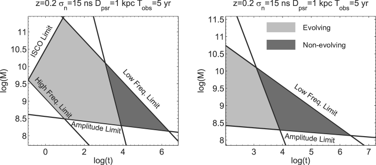
Figure 1: The parameter space of SMBHBs as detectable GW sources for a PTA. The right panel shows an enlarged region of the left panel. The x-axis is the time span from the ‘present’ to the final merger in years; the y-axis is the chirp mass of the SMBHB system in Solar masses. The corresponding limits are labeled on the line, i.e. ‘Amplitude Limit’ for equation. (6), ‘Low Freq. Limit’ and ‘High Freq. Limt’ for equation.  (7), and ‘ISCO Limit’ for equation. (9). The parameter space for evolving and non-evolving GW sources is shaded using using light gray and dark gray respectively as indicated in the figure. It should be noted that, although the dark gray region may look smaller than the light gray region, the dominant detectable SMBHB population belongs to the dark gray region, where we encounter smaller mass and longer rest lifetimes. For our calculations we considered SMBHBs with a and assumed bi-weekly observations of a PTA with 20 pulsars, of which the parameters are shown above the panels.

3 Ability of a PTA to measure the parameters of a non-evolving SMBHB

In the previous section, we estimated the parameter space for the PTA-detectable SMBHB population. In this section, we turn to a detailed analysis of the GW parameter estimation problem. We firstly calculate the pulsar timing response to a monochromatic GW, before we determine the statistical error of estimating GW parameters.

3.1 Pulsar timing signal with a monochromatic GW

Signals in pulsar TOA data come from many different origins, which include the motion of the Earth, the motion of the pulsar (in particular if it is in a binary system), changing relativistic delays in the signal propagation, the scattering, and the dispersing due to space plasma, the gravitational waves in the space time background, etc. (Manchester & Taylor, 1977; Backer & Hellings, 1986; Stairs, 2003; Lorimer & Kramer, 2005). We are, here, particularly interested in the timing signal components related to gravitational waves.

A persistent GW introduces two different signal components in TOA data, i.e. the “Earth term” and the “pulsar term”, where the Earth term depends on the GW strain at the Earth and the pulsar term contains the GW strain at the pulsar. Due to the phase coherence, the Earth term and the pulsar term interfere with each other depending on the pulsar distance, the pulsar direction, and the gravitational wave propagating direction. Because of such pulsar-Earth term interference, the pulsar distance also becomes an important variable in the GW detection problem. The most relevant pulsar timing signals are then the GW induced signal $R_{\rm g}$, the pulsar timing parallax $R_{\rm par}$, and the noise $n$ which includes other noise contributions to the TOAs. Both GW-induced signal and timing parallax depend on the pulsar distances. The timing residual signal can be written as

$$R(t)=T_{0}+P_{0}N+\frac{1}{2}P_{0}\dot{P_{0}}N^{2}+\Delta_{\sun}+R_{\rm g}(t)+R_{\rm par}(t)+n(t|\sigma_{\rm n})\;,$$ (10)

where the $N$ is the sequential pulse number, the $T_{0},P_{0},\dot{P_{0}}$ is the initial epoch, period and period derivative for the pulsar, while $\Delta_{\sun}$ represents the standard Solar system correlations (Lorimer & Kramer, 2005). The $n(t|\sigma_{\rm n})$ is taken to be white zero-mean Gaussian random variables with an RMS level of $\sigma_{\rm n}$ to simulate the other noise contributions to the TOA. In our calculation, we fit for $P_{0}$, $\dot{P_{0}}$, and pulsar sky position using a least-square fitting as in standard pulsar timing pipelines (Lorimer & Kramer, 2005).

As shown in Appendix A, the pulsar timing signal induced by a single GW source is

$$R_{\rm g}(t) = \frac{h_{0}}{2\omega_{\rm g}}\,\frac{\sin(\Delta\Phi/2)}{1-\cos\theta}\left\{\left[B_{1}\cos(2\phi)+B_{2}\sin(2\phi)\right]\cos(\omega_{\rm g}t-\Delta\Phi/2)(1+\cos^{2}\iota)\right.$$ (11)

$$\left.+2\left[B_{2}\cos(2\phi)-B_{1}\sin(2\phi)\right]\sin(\omega_{\rm g}t-\Delta\Phi/2)\cos\iota\right\}\;,$$

where the $B_{1}$, $B_{2}$ and $\Delta\Phi$ depend on the geometrical configuration of the pulsar and GW position by

$$B_{1} = (1+\sin^{2}\beta)\,\cos^{2}\beta_{\rm p}\cos[2(\lambda-\lambda_{\rm p})]-\sin(2\beta)\sin(2\beta_{\rm p})\cos(\lambda-\lambda_{\rm p})+(2-3\cos^{2}\beta_{\rm p})\cos^{2}\beta\;,$$ (12)

$$B_{2} = 2\cos\beta\sin(2\beta_{\rm p})\sin(\lambda-\lambda_{\rm p})-2\sin\beta\cos^{2}\beta_{\rm p}\sin[2(\lambda-\lambda_{\rm p})],$$ (13)

$$\Delta\Phi = \omega_{\rm g}D_{\rm psr}(1-\cos\theta)\;.$$ (14)

Here, the $\lambda$ and $\beta$ are the ecliptic longitude and latitude of the GW source, the $\lambda_{\rm p},\beta_{\rm p}$ are the ecliptic longitude and latitude for the pulsar position, the angle $\iota$ is the orbital inclination of the GW binary source, i.e. the angle between orbital angular momentum and the direction to the Earth. The $h_{0}=2^{4/3}{\cal M}^{5/3}\omega_{\rm g}^{2/3}D_{c}^{-1}(1+z)^{2/3}$ is the GW amplitude.

For a persistent GW source, the pulsar term and the Earth term are coherent and have a phase difference of $\Delta\Phi$. Such pulsar-Earth interference leads to two consequences: 1) it changes the amplitude of the timing signal; 2) it changes the phase of the timing signal. One can see the two effects from equation. (11). The $\sin(\Delta\Phi/2)$ term is the modulation for the signal amplitude, while the $\Delta\Phi/2$ in the term $\omega_{\rm g}t-\Delta\Phi/2$ is the signal phase shift (see Appendix A for the details).

The pulsar timing response $H$ to the GW signal is the normalized ratio between the amplitude of GW-induced pulsar timing signal and the amplitude of the GW, i.e.

$$H = \frac{(\textrm{GW induced amplitude in TOA})\times(\textrm{GW angular frequency})}{(\textrm{GW amplitude})}$$ (15)

$$= \frac{\omega_{\rm g}}{h_{0}}\left[\lim_{T\to\infty}\left(\frac{1}{T}\int_{0}^{T}R_{\rm g}^{2}(t)\,dt\right)\right]^{1/2}\;=\quad\frac{\sin(\Delta\Phi/2)}{4(1-\cos\theta)}\sqrt{B_{3}},$$

where

$$B_{3} = (B_{1}^{2}+B_{2}^{2})(1+6\cos^{2}\iota+\cos^{4}\iota)+\left[(B_{1}^{2}-B_{2}^{2})\cos(4\phi)+2B_{1}B_{2}\sin(4\phi)\right]\sin^{4}\iota.$$ (16)

The response $H$ is a function of the GW source position, the pulsar location, and the orientation of the SMBHB orbit. Due to the interference between the pulsar term and the Earth term, the response $H$ also depends on the distance of the pulsar through the term $\sin(\Delta\Phi/2)$ in equation. (15). Figure 2 shows the timing response as a function of $\theta$, the angle between pulsar direction and GW source direction. The response $H(\theta)$ is simply the response pattern for a single-pulsar GW detector. As shown in Figure 2, the response pattern is made up by a large number of spiky lobes. The envelope of these lobes depends on the GW source position and polarization, and the spiky lobes are due to the interference between the pulsar and the Earth term. Given the angular frequency of the GW $\omega_{\rm g}$ and the pulsar-Earth distance $D_{\rm psr}$, one can show that the angular width of the each lobe is approximately $\theta_{\rm lobe}\sim 1/(2D_{\rm psr}\omega_{\rm g})$ ignoring the weak dependence on $\theta$. For practical PTA purposes, the $D_{\rm psr}\sim 1$ kpc and $\omega_{\rm g}\sim$ yr^-1, so $\theta_{\rm lobe}\sim 10^{-3}$ rad. It is the existence of these spiky lobes which gives PTA experiments the power to accurately locate single GW sources, given that the pulsar distances are well measured.

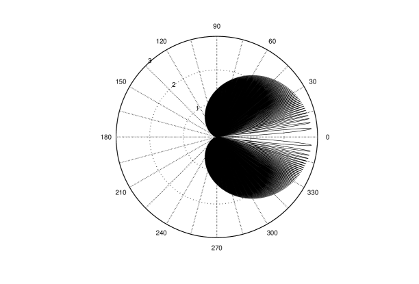
Figure 2: Response pattern $H$ of a single-pulsar timing response to a single monochromatic GW source. For illustration purposes, the pulsar distance is chosen to be small with a value of 200 pc and the GW period is chosen as 5 years, in order to show the structure of the response pattern. The GW source is in the $0^{\circ}$ angle position, the orbital plane inclination is $90^{\circ}$ and the orbital plane coincides with the paper plane. In this way the plotted response pattern is, in fact, the term $(1+\cos\theta)\sin(\Delta\Phi/2)$ in equation. (27).

By measuring the phase difference $\Delta\Phi$ between the pulsar term and the Earth term and by comparing data from different pulsars, the pulsar distance can be inferred. However, the result of such a calculation would have multiple solutions, i.e. we cannot discriminate between the case of $\Delta\Phi$ and the cases of any $\Delta\Phi+4n\pi$, where $n=0,1,2,\dots$, since we have shown in equation. (11) that the GW-induced timing signal $R_{\rm g}$ is a periodical function of $\Delta\Phi$ with a periodicity of $4\pi$. In this way, one can only measure the modulo of the pulsar distance by $4\pi\omega_{\rm g}^{-1}(1-\cos\theta)^{-1}$. On the other hand, if there is another, independent way of measuring the pulsar distance, even with a lower but sufficient accuracy to remove such confusion about multiple solutions, one can use the GW signal to increase the accuracy of pulsar distance measurements by utilizing the GW distance modulo.

For millisecond pulsars, such an independent distance measurements is available from the timing parallax (Backer & Hellings, 1986; Ryba & Taylor, 1991; Lorimer & Kramer, 2005; Verbiest et al., 2010). It is expected that with future radio telescopes, such as the SKA (Kramer & Stappers, 2010; Smits et al., 2010), timing parallax measurements will yield very precise distances for nearby pulsars. Indeed, SKA timing parallax measurements promise to be of sufficient accuracy to help us to identify the correct solution for $\Delta\Phi$ and, hence, to measure the pulsar distance with even better precision.

In order to consider this further, we study a simplified version of the timing parallax term. In reality, the timing parallax is derived from the detailed motion of the Earth from Solar System dynamics (Seidelmann, 2005). For the purpose of this paper, it is sufficient to keep the leading term of the timing parallax, i.e. assuming a circular motion of the Earth,

$$R_{\rm par}(t)=\frac{\cos[2(\lambda_{\rm psr}-\lambda_{\earth}(t))]\cos^{2}\beta_{\rm psr}r_{\earth}^{2}}{4D_{\rm psr}}\;,$$ (17)

where the term $r_{\earth}$ is the average distance between the Sun and the Earth, and $\lambda_{\earth}(t)=2\pi(t/1\,{\rm year})$ is the ecliptic longitude of the Earth at time $t$. This form of timing parallax assumes that the eccentricity of the Earth orbit is zero. This assumption is valid for cases where the pulsar is not too close to the ecliptic poles, i.e. ($-89^{\circ}\leq\beta\leq+89^{\circ}$), such that a timing parallax signal is not dominated by the Earth orbit’s eccentricity. As this will generally be the case, the error of the measured pulsar timing parallax distance is (see Appendix B for details)

$$\sigma_{D_{\rm psr}}=\frac{4\sqrt{2}\,\sigma_{\rm n}D_{\rm psr}^{2}}{\sqrt{N_{\rm obs}}\,r_{\earth}^{2}\cos^{2}\beta_{\rm psr}}\simeq\frac{2.34}{\cos^{2}\beta_{\rm psr}}\left(\frac{N_{\rm obs}}{100}\right)^{-\frac{1}{2}}\left(\frac{D_{\rm psr}}{1\,{\rm kpc}}\right)^{2}\left(\frac{\sigma_{\rm n}}{10\,{\rm ns}}\right)\,{\rm pc}\;,$$ (18)

where $N_{\rm obs}$ is the number of TOAs. The numerical factor is derived assuming that the time span of pulsar data is longer than one year. In a real data analysis, one always uses the full Solar System ephemeris. We compared equation. (18) with results from numerical simulations based on TEMPO and the planetary ephemeris DE405 (Standish, 1998). For pulsars with $-89^{\circ}\leq\beta\leq+89^{\circ}$, we find that the simplified version of the timing parallax shown above agrees with the correct result derived from TEMPO within a few percent difference, justifying the usage of equation. (18) for the purpose of the present paper. We note that the validity of equation. (17) comes from the fact that the Earth orbital eccentricity is small and that we are investigating measurement accuracies, where the effect of orbital eccentricity is of even higher order. According to equation. (18), with a timing accuracy at the 10 to 30-ns level, one can use the timing parallax to measure the pulsar distance accurately to a few light years for pulsar distances of less than 1 kpc. This distance accuracy become comparable to the wavelength of the GW, and the timing parallax measurement is therefore indeed a potential technique to remove the pulsar distance confusion. Both GW parameters and pulsar distances should thus be estimated from pulsar timing data at the same time. In the following, we estimate the corresponding accuracy of the GW parameters and pulsar distances measurements based on the signal timing of equation. (10).

3.2 Vector Ziv-Zakai bound for signals with additive white Gaussian noise

We are, now, going to determine the statistical error of estimating GW parameters using data from a PTA. A well known and popular statistical technique to calculate such lower bounds of the statistical accuracies of parameter estimators is the Cramer-Rao bound (CRB) based on the Fisher information (Fisz, 1963). However CRB is also known for predicting a too small value, which can not be achieved in practical cases, especially, when the signal-to-noise ratio (SNR) is low (Chazan et al., 1975; Bell et al., 1994, 1996; Nicholson & Vecchio, 1998; Van Trees & Bell, 2007). Besides the low-SNR problem, the CRB is derived in the local sense, which assumes that an unbiased estimator (UBE) exists (Fisz, 1963). Due to this assumption, the CRB is not applicable to cases, where the UBE does not exist (Jaynes, 2003). For example, CRB predicts smaller-than-achievable bounds, when there are multiple isolated regions with similar likelihoods in the parameter space. In the present GW parameter estimation problem, the pulsar distance confusion introduces multiple equal-likelihood structures for both pulsar distances and GW source locations at low SNR. This urges us to use, instead of CRB, other techniques to overcome these difficulties. Many statistical bounds were investigated in the passed decades (see Van Trees & Bell (2007) for a review). It turns out that a group of statistical bounds, which originates from Chazan et al. (1975), gives more reliable bounds than the CRB; and these bounds approach the CRB when the SNR is high and multiple equal-likelihood confusions are resolved. These bounds are now referred to as Ziv-Zakai (ZZ) bounds. In this paper, we adopt the ZZ bounds to investigate the error performance of the GW parameter estimators. We also calculate the same results using CRB for comparing purposes.

For a $k$-dimensional vector parameter $\lambda_{i}$ ($i=1\ldots k$), and its estimator $\hat{\lambda}_{i}$, the estimation error is quantified by the correlation matrix ${\cal C}_{ij}=\langle(\hat{\lambda}_{i}-\lambda_{i})(\hat{\lambda}_{j}-\lambda_{j})\rangle$. The error for the estimator $\hat{\lambda}_{i}$ is just the diagonal part of the correlation matrix, i.e. $\sigma_{\lambda_{i}}^{2}={\cal C}_{ii}$. The ZZ bound states that the following inequality holds

$$\kappa_{i}{\cal C}_{ij}\kappa_{j}\geq\frac{1}{2}\int_{\Omega_{\eta}}{\cal V}\left\{\max_{\kappa_{i}\delta\lambda_{i}=\eta}\left[\int[P_{\lambda_{0,i}}(\lambda_{i})+P_{\lambda_{0,i}}(\lambda_{i}+\delta\lambda_{i})]P_{\epsilon,{\rm min}}(\lambda_{i},\lambda_{i}+\delta\lambda_{i})\,d\lambda_{i}\right]\right\}\eta\,d\eta\;,$$ (19)

where $\kappa_{i}$ can be any constant vector. Following the Einstein summation convention, we sum over the index if it appears twice in a single term. The $P_{\lambda_{0,i}}(\lambda_{i})$, $P_{\lambda_{0,i}}(\lambda_{i}+\delta\lambda_{i})$ are the prior probabilities for parameters $\lambda_{i}$ and $\lambda_{i}+\delta\lambda_{i}$ given that the true value of the parameters are $\lambda_{0,i}$. The $\delta\lambda_{i}$ is a $k$-dimensional vector, which maximizes the integral in the rectangular bracket under the constrain that $\kappa_{i}\delta\lambda_{i}=\eta$ in equation. (19), where $\eta$ is the scalar parameterizing the integral path. The $P_{\epsilon,{\rm min}}(\lambda_{i},\lambda_{i}+\delta\lambda_{i})$ is the minimal probability of making an error, when discriminating between the parameter set $\lambda_{i}$ and $\lambda_{i}+\delta\lambda_{i}$. The scalar function $\cal V$ is the ‘valley-filling function’ defined as

$${\cal V}[f(\eta)]=\max_{\eta^{\prime}\geq 0}f(\eta+\eta^{\prime})\;.$$ (20)

The integration domain $\Omega_{\eta}$ is determined by prior information. For example, we may use the fact that the PTA pulsars are all located in the Galaxy, which allows us to confine the integrations for the pulsar distances to the radial size of the Galaxy. We refer to Bell et al. (1994) for details of the formalism in the above. If $\kappa_{i}$ is taken to be the $k$-dimensional unit vector, equation. (19) gives the bounds for the parameter estimation errors. We present more details on how we calculate the Ziv-Zakai bound for our problem in Appendix C.

In order to demonstrate why the ZZ bound is more trustful than classical CRB, we take the GW source position as an example. In Figure 3, we show the $P_{\epsilon,{\rm min}}$ as a function of GW source location. For the case when the GW amplitude is low, there is a high probability of making a mistake in discriminating between the true GW source location and other locations in multiple isolated regions. The CRB is flawed by the large local derivative near the most probable value and it thus underestimates the error by ignoring other isolated high likelihood regions. The ZZ bound, unlike CRB, is an average of the parameter distance $\eta$ weighted by the error probability $P_{\rm\epsilon,min}$ over the entire parameter space. Thus, we only consider the ZZ bound to be suitable for a correct treatment of cases with potential multiple solution confusion.

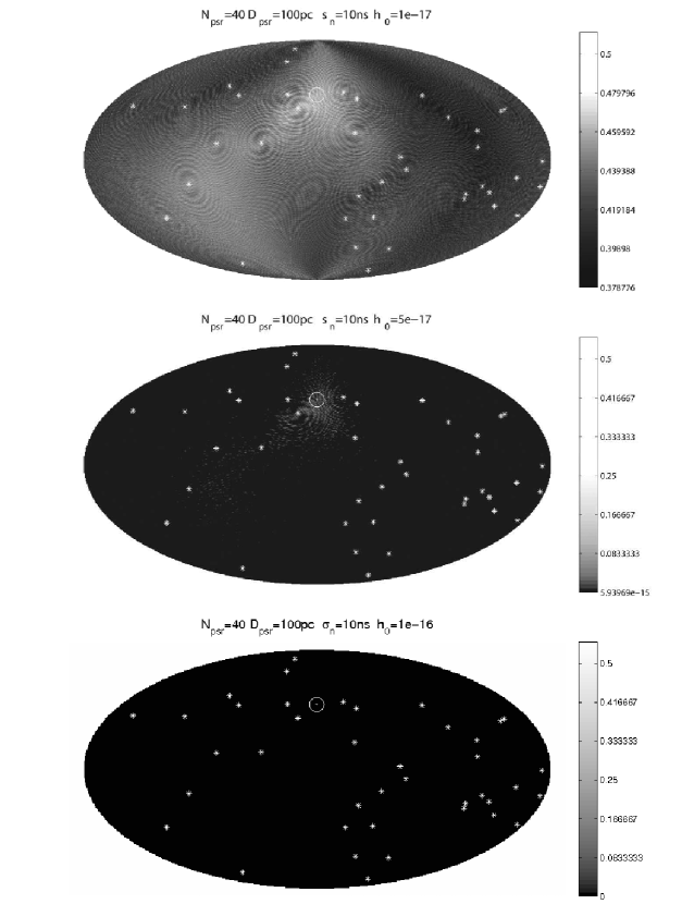
Figure 3: The minimal probability of incorrectly determining the source location. Here, the GW source is located at the center of the white circle. The gray scale shows the minimal probability of making a mistake ($P_{\epsilon,{\rm min}}$) when deciding between the true GW source location and any other location in the $\lambda-\beta$ parameter space. When the GW amplitude is low (top panel), $P_{\rm\epsilon,min}$ is large ($\simeq 0.5$) over the whole sky. When the GW amplitude is strong enough (bottom panel), the probability of determining an incorrect GW location is lower and the multiple-solution confusion is removed. Thus only the real GW position is left. For intermediate GW amplitudes (middle panel), there are multiple isolated positions, which all have high probability of being indistinguishable from the true GW source position. For the illustration purpose here, these figures are calculated for a PTA with 40 pulsars, where each pulsar has a 10-ns timing accuracy and a distance of 100 pc. The GW frequency is taken to be $1.2$ year. The white stars indicate the locations of the PTA pulsars. The visible interference pattern is due to the response pattern discussed in the text.

Since we are interested in calculating the errors of the estimated GW source parameters as functions of the GW and pulsar parameters, the priors $P_{\lambda_{0,i}}(\lambda_{i})$ and $P_{\lambda_{0,i}}(\lambda_{i}+\delta\lambda_{i})$ take forms of Dirac $\delta$-functions, i.e. $P_{\lambda_{0,i}}(\lambda_{i})=P_{\lambda_{0,i}}(\lambda_{i}+\delta\lambda_{i})=\delta(\lambda_{i}-\lambda_{0,i})$, where $\lambda_{0,i}$ is the true parameter. With the pulsar signal model specified by equation. (10), one can calculate the ZZ bound for the parameter estimators, i.e. for the pulsar distance $D_{\rm psr}$ and the GW parameters $h_{0},\iota,\lambda,\beta,\phi,\omega_{\rm g},\phi_{0}$. For a PTA with $N_{\rm psr}$ pulsars, the total number of parameters is $N_{\rm psr}+7$, where the seven represents the GW parameters. Details describing the calculation of the ZZ bounds are given in Appendix C. We present the results in Figures 4, where the errors of the parameter estimators are given as functions of the GW amplitude for various configuration of PTAs. For high-SNR cases, the two bounds (ZZ and CR) agree with each other within the computational accuracy. For intermediate-SNR cases, the ZZ-bound indicates a larger uncertainty than for the CRB predictions. This confirms that the CRB underestimates the parameter errors, which is mainly due to the multiple solution confusions as we discussed before. At the low-SNR limit, the ZZ bound converges to a fixed value because of prior information about $\Omega_{\eta}$, i.e. we made use of the fact that the error of the inclination angle $\iota$ and source position error will not be larger than $2\pi$, and that the error of the GW frequency will not be greater than the sampling frequency. From the results, one can also see that the CRB underestimates the error of the GW source location and GW frequency by one or two orders of magnitudes for intermediate-SNR cases. We conclude that the CRB is indeed not an appropriate tool to investigate the error performance of PTAs as a GW detector, in accordance with the results by Bell et al. (1996).

We present the error of pulsar distance measurements as a function of GW amplitude in Figure 5. As a pulsar distance we use $0.5-1$ kpc. The measurements of the pulsar timing parallax is for the intermediate-SNR case. Again, the CRB and ZZ bounds differ from each other, i.e. CRB underestimates the measurement errors by orders of magnitude.

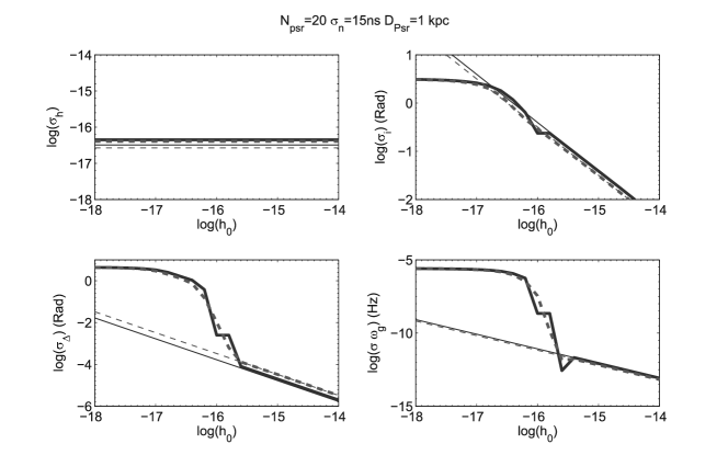
Figure 4: The parameter estimation error as a function of GW amplitude. $\sigma_{\rm h}$ is the lower bound for the accuracy in estimating the GW amplitude $h_{0}$, $\sigma_{\rm i}$ is for the orbital inclination angle of the GW source, $\sigma_{\rm\Delta}=\sqrt{\sigma_{\lambda}^{2}\sin^{2}\beta+\sigma_{\beta}^{2}}$ is the lower bound for the accuracy in measuring the GW source position, where $\sigma_{\lambda}$ and $\sigma_{\beta}$ are the errors for estimating $\lambda$ and $\beta$, respectively. The $\sigma_{\rm\omega_{\rm g}}$ is the lower bound of the measurement accuracy of the GW frequency. The $h_{0}$ is the GW amplitude. One can see that the error of amplitude estimation is not sensitive to the true GW amplitude, while the uncertainties in the other parameters decrease as the GW amplitude becomes larger (Takahashi & Seto, 2002). The thick lines are the results from the ZZ bound, and the thin lines are the bounds calculated from the CRB. The dashed line is for a GW with a period of 2.2 years, while the solid line is for a GW with a 4.4 year period. The total observation span $T$ is 5 years and the duration $\Delta T$ between two successive observation are 2 weeks. The pulsars in the PTA are uniformly distributed over the sky at equal distance. Details about the PTA, such as the number of pulsars, timing precision and pulsar distances are given at the top of the figure.

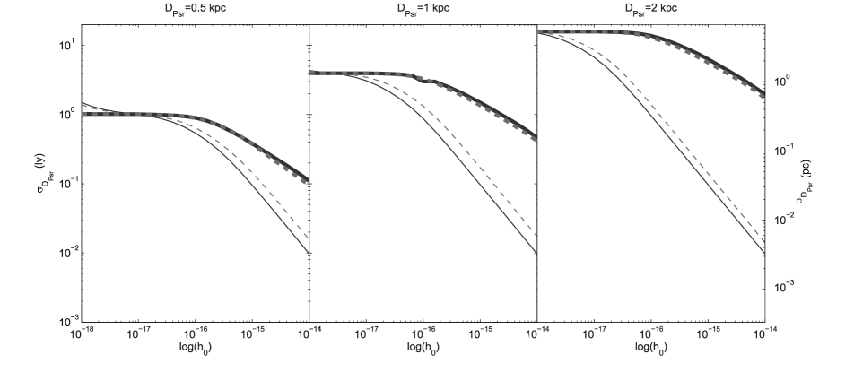
Figure 5: Error for pulsar distance measurements as a function of GW amplitude. With a PTA GW detection, one can measure the distance to the used pulsars with improved accuracy. The left, middle, and right panel correspond to pulsars with distances of 0.5 kpc, 1 kpc, and 2 kpc, respectively. The thick lines (upper two) correspond to the ZZ bound and the thin lines (lower two) correspond to the CRBs. The solid line is for GWs with a period of 2.2 years and the dashed lines is for GWs with a period of 4.4 years. It may be counter intuitive that the ZZ and CRB agree at the low SNR limit. However, this is the consequence of GW-induced multiple solution confusion for pulsar distances as we discussed in the main text. In fact, the difference between ZZ bound and the CRB is due to the GW-induced multiple solution confusion of pulsar distance. Because pulsar timing parallax alone has well defined unbiased estimators, the ZZ bound and the CRB agree with each other when the amplitude of the GW is small and little confusion is introduced.

4 Discussion and Conclusions

In this paper we have shown that we can use a pulsar timing array to detect the non-evolving single gravitational wave sources and measure their physical parameters. One can detect a GW source with a GW amplitude larger than $5\times 10^{-17}$ by timing 20 pulsars bi-weekly (once every two weeks) for 5 years with a timing accuracy of 15 ns. This agrees with the analytical estimation in equation. (5). Such observational requirements (i.e. 15 ns timing accuracy) have not been achieved at present, but should be possible for future radio-astronomical instruments such as the Square Kilometer Array (SKA) and possibly, for a limited number of sources, also for the Five-hundred-meter Aperture Spherical Radio Telescope (FAST) (Nan et al., 2006; Smits et al., 2009; Kramer, 2010). For such large telescope sensitivity, radiometer noise will not be the limiting factor to achieve a 15 ns-level noise budget. Rather, limiting factors may arise from other physical effects, which we will discuss shortly.

In our treatment of single GW source detection, we do the novel step of including the pulsar term as an integral part of the signal that we are looking for. This is possible since the timing parallax offers the possibility of modelling the pulsar terms accurately for nearby sources. We take advantage of the pulsar term in several ways. Firstly, by using the pulsar term, we increase the signal-to-noise ratio (SNR). When the pulsar term is completely ignored, the GW signals (only including Earth terms) in pulsar timing data are sinusoidal waves with identical phases and the pulsar term becomes a noise source with the same amplitude compared to the ‘signal’ term. The SNR of single pulsar data is then always less than one. Even worse, the ignored pulsar-term is sinusoidal signal with unknown phase. It is not a stationary signal. It is only reduced by averaging over multiple pulsars but not by time averaging. On the other hand, if we can use the pulsar term as a ‘signal’ term, we can sum the signal from multiple pulsar coherently and the SNR of single pulsar data can be arbitrarily large, depending on the GW amplitude. The second important benefit of utilizing the pulsar term is that it allows us to get a precise measurement for the GW source location. The interference between the pulsar term and the Earth term introduces spiky lobes in the single-pulsar response pattern (see Figure 2). In Figure 3, where the small scale ring-type structures come from individual response patterns and the large scale quadruple structure is introduced by the coherence of the Earth term. This large scale quadruple structure is, in fact, the response pattern, when one only uses the Earth term as a signal. Clearly the small scale spiky structure increases the locating ability of PTAs substantially and allows astronomers to search of electromagnetic counterparts of the GW source.

Thanks to the pulsar timing parallax signal, we are able to include the pulsar term in our scheme to detect non-evolutionary GW sources. Our method, first presented in Kramer & Stappers (2010), was complemented recently by the work of Corbin & Cornish (2010) who also include the pulsar term in their analysis pipeline. Their approach to use the pulsar term however differs, as they study the chirped signal and ignore the timing parallax signal, while we use the pulsar term in combination with the timing parallax signal.

The pulsar term leads to many potential important applications. For example, Deng & Finn (2010) recently point out that the curvature of the wavefronts introduces a GW parallax effect, which can be used to measure the SMBHB distance. Other possible applications are very interesting to study also. For instance, while the pulsar distance measurement helps the GW detection, the GW signal, on the other hand, also helps the pulsar distance measurement. Due to the interference between the pulsar term and the Earth term, the GW signal is sensitive to the pulsar distance. In this way, the detected GW signal can be used to increase the accuracy of our distance measurements. As we expected, the overall measurement accuracy for pulsar distances increases with GW amplitude, as shown in Figure 5. The improvement in accuracy increases faster with respect to the GW amplitude for pulsars with smaller distances ($D_{\rm psr}=0.5$ kpc) than the ones with larger distances ($D_{\rm psr}=2$ kpc). This is because the distance measurement using the timing parallax has higher precision for near-by pulsars than for far-away pulsars. A smaller number of multiple distance solutions occurs for the nearby pulsars, for which the accuracy of distance measurements increases faster when the GW amplitude becomes larger.

In this paper, we have treated the noise as an additive uncorrelated noise (white noise). Because noise arises from various different sources: 1) the instrumental noise, e.g. clock errors, ephemeris errors, polarimetry calibration errors, radio-frequency interference, etc.; 2) pulsar intrinsic noise, e.g. micro glitch at even smaller level, switch of spin down rate, pulsar profile change, etc.; 3) propagation effects, e.g. DM variation and scattering. Thus the noise is not necessarily white. For a stochastic GW background detection using pulsar timing arrays, a correct treatment of the red noise is a very important issue, since red noise may destroy any measurable correlation function (Jenet et al., 2005). However the red noise issue is less critical for single source detection. This is a consequence of the spectral analysis. Since the signal spectrum for non-evolving SMBH will be a single peak at the GW frequency, the SNR of the detection is basically the ratio between the GW induced signal power and the noise power in the frequency bin (Yardley et al., 2010). Thus, red noise may be dominant at lower frequencies, but less effective in the frequency bin of the signal from a single GW source. This is fundamentally different from the stochastic GW background detection.

Although several pulsars have timing residuals that are essentially white (Verbiest et al., 2009) at the current level of accuracy, it is still an unanswered question as to whether the residuals remain white for much higher timing precision or for much longer observing span. Several authors have modeled the statistics of red noise (Foster & Backer, 1990; Cordes & Shannon, 2010; Shannon & Cordes, 2010), while some works show the potential of improving timing accuracy by introducing corrections to interstellar medium effects (Hemberger & Stinebring, 2008; Demorest, 2010). Indeed, for a few selected pulsars a timing precision at a 30$\sim$50 ns-level (Demorest, 2010) is already possible at present, but further studies are needed to see how and if this can be improved.

Beside pulsar timing parallax techniques, one can also determine pulsar distances from other methods, such as the Very Long Baseline Interferometry (VLBI), pulsar orbital parallax, and relative acceleration (Smits et al., 2010). Since in this paper we mainly focus on extracting GW information and pulsar distances from pulsar timing array data, investigation on incorporating these extra information into PTA GW data analysis will be presented in future studies.

Finally, we have demonstrated how the errors in the parameter estimation can be determined reliably. We have calculated the parameter estimation error using both the CRB and the ZZ bound. Both of the methods give nearly identical results in the high SNR region, as we expected. But the two methods deviate from each other when the SNR is low. The CRB is known to predict unreachable accuracy in the low-SNR regime, while the ZZ bound gives more trustful results in that region. For most applications involving GW detection, the noise contributions dominate above the GW signals, so that the ZZ bound turns out to be superior in reliability compared to the CRB.

Appendix A Pulsar timing residuals induced by a monochromatic GW

In this section we consider a non-evolving binary system in a circular orbit as the source of a monochromatic gravitational wave. If we choose the coordinate system such that the gravitational wave is in the $z$-axis and the ascending node along the $x$-axis (reference frame of the source), the two polarizations can be written as (Blanchet, 2006)

$$h_{+}(t) = h_{0}\cos(\omega_{\rm g}t+\Phi_{0})\,\frac{1+\cos^{2}\iota}{2}\;,$$ (21)

$$h_{\times}(t) = h_{0}\sin(\omega_{\rm g}t+\Phi_{0})\,\cos\iota\;,$$ (22)

$\Phi_{0}$ is a constant phase shift and $\iota$ denotes the angle between the orbital angular momentum of the source and the direction from the source to the Earth. The amplitude $h_{0}$ depends on the binary parameters and distance (see Section 3.1). For a pulsar at distance $D_{\rm psr}$, with azimuthal angle $\psi$ and with polar angle $\theta$, the residuals caused by the gravitational wave are given by (Estabrook & Wahlquist, 1975; Detweiler, 1979; Wahlquist, 1987)

$$R(t)=(1+\cos\theta)\,\left[(H_{+}^{E}-H_{+}^{p})\cos(2\psi)+(H_{\times}^{E}-H_{\times}^{p})\sin(2\psi)\right]\;.$$ (23)

where

$$H_{+}^{E}-H_{+}^{p} = \frac{h_{0}}{2\omega_{\rm g}}\sin(\Delta\Phi/2)(1+\cos^{2}\iota)$$ (24)

$$\qquad\left[\cos(\omega_{\rm g}t+\Phi_{0}-\Delta\Phi/2)-\cos(\Phi_{0}-\Delta\Phi/2)\right]\;,$$

$$H_{\times}^{E}-H_{\times}^{p} = \frac{h_{0}}{2\omega_{\rm g}}\sin(\Delta\Phi/2)(2\cos\iota)$$ (25)

$$\qquad\left[\sin(\omega_{\rm g}t+\Phi_{0}-\Delta\Phi/2)-\sin(\Phi_{0}-\Delta\Phi/2)\right]\;,$$

where

$$\Delta\Phi=\omega_{\rm g}D_{\rm psr}(1-\cos\theta)\;.$$ (26)

After dropping constant terms, the timing residuals caused by the gravitational wave reads

$$R(t) = \frac{h_{0}}{2\omega_{\rm g}}(1+\cos\theta)\sin(\Delta\Phi/2)$$ (27)

$$\left[(1+\cos^{2}\iota)\cos(2\psi)\cos(\omega_{\rm gw}t+\Phi_{0}^{\prime})+2\cos\iota\sin(2\psi)\sin(\omega_{\rm gw}t+\Phi_{0}^{\prime})\right]\;,$$

where $\Phi^{\prime}=\Phi_{0}-\Delta\Phi/2$. One can easily convert these results to the representation in ecliptic coordinates as used in the main text. The representation here has the merit of clearly presenting the physical pictures. For example, it looks like a singularity at $\theta=0$ in equation. (39), but the representation here, equation. (27), clearly shows that the singularity is canceled by geometrical factors of GW polarization. The amplitude modulation ($\sin(\Delta\Phi/2)$) and phase modulation ($\Delta\Phi/2$) can be easily understood using the identity $e^{{\rm i}(\omega t+\Delta\Phi)}-e^{{\rm i}\omega t}=2\sin(\Delta\Phi/2)e^{{\rm i}(\omega t+\Delta\Phi/2+\pi/2)}$, where the interference between two sinusoidal signals with a phase difference of $\Delta\Phi$ introduces an amplitude modulation of $\sin(\Delta\Phi/2)$ and a phase shift of $\Delta\Phi/2+\pi/2$.

One can also calculate the results using the observer frame. The waveform of GWs from a SMBHB with a circular orbit at cosmological redshift $z$ and chirp mass $\cal M$ is given by (Wahlquist, 1987; Blanchet, 2006; Hughes, 2009)

$$h_{ij}=\epsilon_{ij}^{+}A_{+}+\epsilon_{ij}^{\times}A_{\times}\;,$$ (28)

where the $A_{+}$ and $A_{\times}$ are the waveforms of the two polarization modes ‘+’ and ‘$\times$’, respectively. The polarization tensors $\epsilon_{ij}^{+}$ and $\epsilon_{ij}^{\times}$ are (Wahlquist, 1987)

$$\epsilon_{ij}^{+} = \left(\begin{array}[]{ccc}\sin^{2}\lambda-\cos^{2}\lambda\sin^{2}\beta&-\sin\lambda\cos\lambda\left(\sin^{2}\beta+1\right)&\cos\lambda\sin\beta\cos\beta\\ -\sin\lambda\cos\lambda\left(\sin^{2}\beta+1\right)&\cos^{2}\lambda-\sin^{2}\lambda\sin^{2}\beta&\sin\lambda\sin\beta\cos\beta\\ \cos\lambda\sin\beta\cos\beta&\sin\lambda\sin\beta\cos\beta&-\cos^{2}\beta\end{array}\right)\;,$$ (32)

$$\epsilon_{ij}^{\times} = \left(\begin{array}[]{ccc}\sin(2\lambda)\sin\beta&-\cos(2\lambda)\sin\beta&-\sin\lambda\cos\beta\\ -\cos(2\lambda)\sin\beta&-\sin(2\lambda)\sin\beta&\cos\lambda\cos\beta\\ -\sin\lambda\cos\beta&\cos\lambda\cos\beta&0\end{array}\right)\;,$$ (36)

where $\lambda$ and $\beta$ are the ecliptic longitude and latitude of the GW source. For a non-evolving SMBHB with circular orbit, the GW waveform $A_{\times}$ and $A_{+}$ of the two polarization modes are (Wahlquist, 1987)

$$A_{+} = h_{0}\left[\cos\iota\sin(2\phi)\sin(\omega_{\rm g}t)-\frac{1}{2}(1+\cos^{2}\iota)\cos(2\phi)\cos(\omega_{\rm g}t)\right]\;,$$ (37)

$$A_{\times} = -h_{0}\left[\cos\iota\cos(2\phi)\sin(\omega_{\rm g}t)+\frac{1}{2}(1+\cos^{2}\iota)\sin(2\phi)\cos(\omega_{\rm g}t)\right]\;.$$ (38)

The angle $\iota$ is the orbital inclination of the GW binary source, i.e. the angle between orbital angular momentum and the gravitational wave vector. The angle $\phi$ defines the direction of the binary ascending node on the sky. The GW source chirp mass $\cal M$ and the source distance $D_{c}$ degenerate to the GW amplitude $h_{0}$, if one only has the PTA data. Instead of discussing the detection statistics using full GW source parameters (${\cal M},D_{c},\omega_{\rm g}$), it is much better to use the reduced parameter sets ($h_{0},\omega_{\rm g}$), which will be used from now on.

A GW affects the pulsar timing by introducing shifts to the observed rotational frequency of the pulsar, $\nu$ (see refs. Detweiler (1979); Lee et al. (2008), and Appendix A for details)

$$\frac{\delta\nu}{\nu}=-\frac{1}{2}\,\frac{\hat{n}_{i}\hat{n}_{j}}{1-\cos\theta}\left[h_{ij}(t,0)-h_{ij}(t-D_{\rm psr},{\bf D}_{\rm psr})\right]\;,$$ (39)

where $\hat{\rm\bf n}$ is the unit vector pointing from the observer to the pulsar and $\theta$ is the angle between the GW source direction and the pulsar direction for the observer. The $h_{ij}(t,0)$ is the GW strain at the Earth (the introduced Earth term) and the $h_{ij}(t-D_{\rm psr},{\rm\bf D_{\rm psr}})$ is the GW strain at the pulsar (the introduced pulsar term). The explicit forms for $\hat{\rm\bf n}$ and the $\cos\theta$ are

$${\rm\bf\hat{\rm\bf n}} = \left(\begin{array}[]{c}\cos\lambda_{\rm p}\cos\beta_{\rm p}\\ \sin\lambda_{\rm p}\cos\beta_{\rm p}\\ \sin\beta_{\rm p}\end{array}\right)\;,$$ (43)

$$\cos\theta = \cos\beta\cos\beta_{\rm p}\cos(\lambda-\lambda_{\rm p})+\sin\beta\sin\beta_{\rm p}$$ (44)

where $\lambda_{\rm p},\beta_{\rm p}$ are again the ecliptic longitude and latitude for the pulsar position.

The GW induced TOA signal $R_{\rm g}(t)$ is the integration of the frequency shift over the observer’s local time, $R_{\rm g}(t)=\int\frac{\delta\nu(t)}{\nu}\,dt$ (Jenet et al., 2005). Inserting equation. (37) and equation. (38) into Equation. (28) and integrating equation. (39) over time yields Equation, (11).

Appendix B Analytical calculation for the errors of timing parallax measurements

In this section, we derive an analytic expression for the uncertainty in the distance measurement for pulsars using the timing parallax. As a first-order approximation, we assume that the Earth follows a circular orbit. In practice, the Earth orbit is not only eccentric, but also shows additional, quite complex deviations from an elliptical orbit due to perturbations by other masses in the Solar System. However, because the eccentricity of the Earth orbit is small, and we only need a first order estimation of the error in the parallax measurement, our assumption is justified. A more complete discussion on pulsar timing parallax measurements can be found in the literature (Backer & Hellings, 1986; Ryba & Taylor, 1991; Lorimer & Kramer, 2005).

We assume that the pulsar TOA signal is composed of the timing parallax term and a white Gaussian noise term representing noise contributions from other processes, i.e.

$$R(t)=R_{\rm par}(t)+n(t)\;.$$ (45)

Regarding the time series of signals as a vectors, e.g. ${\rm\bf R}=R(t_{i})$, $i=1\ldots N_{\rm obs}$, where the $N_{\rm obs}$ is the number of data points and $t_{i}$ is the time of the $i$-th observation. The probability distribution, $f({\rm\bf R}|D_{\rm psr})$, for the TOA data $\rm\bf R$, with given pulsar distance $D_{\rm psr}$, is

$$f({\rm\bf R}|D_{\rm psr})=\left(\frac{1}{\sqrt{2\pi}\sigma_{\rm n}}\right)^{N_{\rm obs}}{\rm Exp}\left[-\sum_{i=1}^{N_{\rm obs}}\frac{\left[R(t_{i})-R_{\rm par}(t_{i})\right]^{2}}{2\sigma_{\rm n}^{2}}\right]\;.$$ (46)

Using the CRB, the uncertainty of pulsar distance measurements is

$$\sigma_{D_{\rm psr}}^{2}\leq\frac{1}{{\int}\!\left[\frac{\mathrm{d}\ln f({\rm\bf R}|D_{\rm psr})}{\mathrm{d}D_{\rm psr}}\right]^{2}f({\rm\bf R}|D_{\rm psr})\,\mathrm{d}{\rm\bf R}}\;,$$ (47)

which corresponds to equation. (18) of the main text. We have checked this result against simulations with the pulsar timing software TEMPO, which uses the planetary ephemeris DE405 for a highly accurate representation of the Earth orbit in the Solar System barycenter. For pulsars which are not too close to the poles of the ecliptic (more than one degree angular distance), our analytic equation (46) agrees to better than a few percent.

Appendix C Ziv-Zakai bounds for array signal with additive noise

The ZZ bound was first introduced for a scalar parameter estimation problem by Chazan et al. (1975), and was later extended to general vector parameter estimation problems (Bell et al., 1994). Its first use for GW studies was by Nicholson & Vecchio (1998). In this paper, we only summarize the key results of the ZZ bound and refer readers to the literatures cited for further information.

We suppose that we are dealing with timing data from an array of $N_{\rm psr}$ pulsars. The data of each pulsar is a $N$-point TOA serial signal. We denote the whole timing data set by $R_{j}^{i}$, where the superscript is the pulsar index, and the subscript is the data index. For example, the $R_{j}^{i}$ is the $j$-th data point of the $i$-th pulsar TOA. The timing data is just a $N_{\rm psr}$-times-$N$ dimensional vector ${\rm\bf R}$ and their components $R_{j}^{i}$ takes the form of equation. (10). The signal part of $\rm\bf R$ is completely determined by the $k$-dimensional parameter $\lambda_{k}$ (GW parameters plus pulsar parameters). The noise part is a random variable following independent Gaussian statistics. We have

$$R_{j}^{i}=s_{j}^{i}(\lambda_{k})+n_{j}^{i},$$ (48)

where the signal part ${\rm\bf s}={\rm\bf R}_{\rm g}+{\rm\bf R}_{\rm par}$, and the noise $\rm\bf n$ is assumed to be an un-correlated white Gaussian noise, i.e. $\langle n_{j}^{i}n_{j}^{i}\rangle=\sigma_{\rm n}^{2\;(i)}$ and $\langle n_{j^{\prime}}^{i}n_{j}^{i^{\prime}}\rangle=0$ for any $j^{\prime}\neq j$ or $i^{\prime}\neq i$. The $\sigma_{\rm n}^{(i)}$ is the RMS level for the $i$-th pulsar TOA noise from other contributions. The $P_{\epsilon,{\rm min}}(\lambda_{k},\lambda_{k}^{\prime})$ is the minimal probability of making a mistake in deciding which parameter set, the $\lambda_{k}$ or $\lambda_{k}^{\prime}$, to choose, when giving data ${\rm\bf R}$. For the case where $\rm\bf\lambda$ and $\rm\bf\lambda^{\prime}$ have equal prior, as shown by Kassam (1988), the following likelihood ratio test minimizes the probability of making mistakes,

$$\textrm{choose }\left\{\begin{array}[]{c}\lambda_{k}\textrm{, if }\frac{f({\rm\bf R}|\lambda_{k})}{f({\rm\bf R}|\lambda_{k}^{\prime})}>1\\ \lambda_{k}^{\prime}\textrm{, if }\frac{f({\rm\bf R}|\lambda_{k})}{f({\rm\bf R}|\lambda_{k}^{\prime})}<1\end{array}\right.,$$ (49)

where the $f({\rm\bf R}|\lambda_{k})$ is the probability distribution function of the data ${\rm\bf R}$, when the parameters take value of $\lambda_{k}$. Following the likelihood test in equation. (49), one can show

$$P_{\epsilon,{\rm min}}(\lambda_{k},\lambda_{k}^{\prime})=\frac{1}{2}\left[P\left(\left.\frac{f({\rm\bf R}|\lambda_{k})}{f({\rm\bf R}|\lambda_{k}^{\prime})}>1\right|\lambda_{k}^{\prime}\right)+P\left(\left.\frac{f({\rm\bf R}|\lambda_{k})}{f({\rm\bf R}|\lambda_{k}^{\prime})}<1\right|\lambda_{k}\right)\right].$$ (50)

For the uncorrelated white Gaussian noise, the likelihood ratio $f({\rm\bf R}|\lambda_{k})/f({\rm\bf R}|\lambda_{k}^{\prime})$ is

$$\left.\frac{f({\rm\bf R}|\lambda_{k})}{f({\rm\bf R}|\lambda_{k}^{\prime})}\right|_{\lambda_{0,k}}=\frac{{\rm Exp}\left[{-\sum_{i=1}^{N_{\rm psr}}\sum_{j=1}^{N}\left(s_{j}^{i}(\lambda_{0,k})-s_{j}^{i}(\lambda_{k})+n_{j}^{i}\right)^{2}/\left(2\sigma_{n}^{2\;(i)}\right)}\right]}{{\rm Exp}\left[{-\sum_{i=1}^{N_{\rm psr}}\sum_{j=1}^{N}\left(s_{j}^{i}(\lambda_{0,k})-s_{j}^{i}(\lambda_{k}^{\prime})+n_{j}^{i}\right)^{2}/\left(2\sigma_{n}^{2\;(i)}\right)}\right]}.$$ (51)

Integrating over the random vectors $n_{j}^{i}$, one derives

$$P\left(\left.\frac{f({\rm\bf R}|\lambda_{k})}{f({\rm\bf R}|\lambda_{k}^{\prime})}>1\right|\lambda_{0,k}\right)=\frac{1}{2}{\rm Erfc}\left[-\frac{\sum_{i=1}^{N_{\rm psr}}\frac{1}{\sigma_{\rm n}^{2\;i}}\sum_{j=1}^{N}(s_{j}^{i}(\lambda_{0,k})-s_{1}^{i})(s_{j}^{i}(\lambda_{k})-s_{j}^{i}(\lambda_{k}^{\prime}))}{\sqrt{2}\sqrt{\sum_{i=1}^{N_{\rm psr}}\frac{1}{\sigma_{\rm n}^{2\;(i)}}\sum_{j=1}^{N}\left(s_{j}^{i}(\lambda_{k})-s_{j}^{i}(\lambda_{k}^{\prime})\right)^{2}}}\right],$$ (52)

and the $P\left(\left.\frac{f({\rm\bf R}|\lambda_{k})}{f({\rm\bf R}|\lambda_{k}^{\prime})}<1\right|\lambda_{0,k}\right)$ can be evaluated in very similar fashion. The minimal error probability $P_{\epsilon,{\rm min}}$ is then

$$P_{\epsilon,{\rm min}}(\lambda_{k},\lambda_{k}^{\prime})=\frac{1}{2}{\rm Erf}(\zeta),$$ (53)

where

$$\zeta=\sqrt{\sum_{i=1}^{N_{\rm psr}}\frac{\sum_{j=1}^{N}\left[s_{j}^{i}(\lambda_{k})-s_{j}^{i}(\lambda_{k}^{\prime})\right]^{2}}{2\,\sigma_{\rm n}^{2\;(i)}}}.$$ (54)

equation. (54) and (53) show that the larger difference between the signal of $\lambda_{k}$ and the signal of $\lambda_{k}^{\prime}$, the larger $\zeta$ is, and the less probability one will make a mistake in discriminating between the two signals.

Appendix D Generalization of the amplitude condition to the red noise case

In the main text, equation (5) is valid only for white-nosie. Since equation (5) is quite useful to estimate the detectable amplitude of monochromatic GWs, we generalize it here also for the red-noise case. The easiest way of deriving equation (5) is by using a spectral analysis in frequency space.

We focus on the frequency bin, which contains the GW signal, i.e. the frequency band of $[f-\frac{1}{2}\Delta f,f+\frac{1}{2}\Delta f]$. For signals from $N_{\rm psr}$ pulsars, the total GW signal power $P_{\rm s}$ in the frequency bin is

$$P_{\rm s}=\left(\frac{N_{\rm psr}\overline{h}}{2\omega_{\rm g}}\right)^{2}\,,$$ (55)

and the noise power is

$$P_{\rm n}=N_{\rm psr}S_{n}(f)\Delta f=\frac{N_{\rm psr}S_{n}(f)f_{\rm max}}{N_{\rm obs}}\,,$$ (56)

where the $S_{n}(f)$ is the spectra of $n(t)$, the noise component. The $f_{\rm max}$, defined in Section 2, is the bandwidth of the signal. The detectable condition is then $P_{\rm s}\geq P_{\rm n}$, which leads to

$$\frac{\overline{h}}{2\omega_{\rm g}}\geq\sqrt{\frac{S_{\rm n}(f)f_{\rm max}}{N_{\rm psr}N_{\rm obs}}}\,.$$ (57)

In this way, the generalization of equation (5) to the red-noise case is simply to replace the RMS noise level $\sigma_{\rm n}$ with the value of $\sigma_{\rm e}=\sqrt{S_{\rm n}(f)f_{\rm max}}$, the effective level of noise.

References

- Backer & Hellings (1986) Backer D. C., Hellings R. W., 1986, ARA&A, 24, 537
- Bell et al. (1996) Bell K. L., Ephraim Y., van Trees H. L., 1996, IEEE Transactions on Signal Processing, 44, 2810
- Bell et al. (1994) Bell K. L., Steinberg Y., Ephraim Y., 1994, IEEE Transactions on Information Theory, p. 75
- Bertotti et al. (1983) Bertotti B., Carr B. J., Rees M. J., 1983, MNRAS, 203, 945
- Blanchet (2006) Blanchet L., 2006, Living Reviews in Relativity, 9, 4
- Blanchet & Iyer (2003) Blanchet L., Iyer B. R., 2003, Classical and Quantum Gravity, 20, 755
- Blandford et al. (1984) Blandford R., Romani R. W., Narayan R., 1984, Journal of Astrophysics and Astronomy, 5, 369
- Burke-Spolaor (2010) Burke-Spolaor S., 2010, arxiv: 10084382, to apprear in MNRAS
- Burt et al. (2010) Burt B. J., Lommen A. N., Finn L. S., 2010, arxiv: 10055163
- Chazan et al. (1975) Chazan D., Zakai M., Ziv J., 1975, IEEE Transactions on Information Theory, 21, 90
- Corbin & Cornish (2010) Corbin V., Cornish N. J., 2010, arxiv: 10081782
- Cordes & Shannon (2010) Cordes J. M., Shannon R. M., 2010, arxiv: 10103785
- Cutler & Thorne (2001) Cutler C., Thorne K., 2001, in Proceedings of the GR16 2001. Durban, South Africa An Overview of Gravitational-Wave Sources
- Demorest (2010) Demorest P. B., 2010, in Proceedings of the Pulsar Conference 2010. Sardinia, Italy., High precision timing of millisecond pulsars at arecibo and green bank
- Deng & Finn (2010) Deng X., Finn L. S., 2010, arxiv: 10080320
- Detweiler (1979) Detweiler S., 1979, ApJ, 234, 1100
- Estabrook & Wahlquist (1975) Estabrook F. B., Wahlquist H. D., 1975, General Relativity and Gravitation, 6, 439
- Finn & Lommen (2010) Finn L. S., Lommen A. N., 2010, ApJ, 718, 1400
- Fisz (1963) Fisz M., 1963, Probability Theory and Mathematical Statistics . New Yorker: Wiley
- Foster & Backer (1990) Foster R. S., Backer D. C., 1990, ApJ, 361, 300
- Hellings & Downs (1983) Hellings R. W., Downs G. S., 1983, ApJL, 265, L39
- Hemberger & Stinebring (2008) Hemberger D. A., Stinebring D. R., 2008, ApjL, 674, L37
- Hobbs et al. (2009) Hobbs G., Jenet F., Lee K. J., Verbiest J. P. W., Yardley D., Manchester R., Lommen A., Coles W., Edwards R., Shettigara C., 2009, MNRAS, 394, 1945
- Hughes (2009) Hughes S. A., 2009, ARA&A, 47, 107
- Jaynes (2003) Jaynes E. T., 2003, Probability Theory: The Logic of Science (Vol 1). Cambridge Univ. Press., Cambridge, UK
- Jenet et al. (2005) Jenet F. A., Hobbs G. B., Lee K. J., Manchester R. N., 2005, ApJL, 625, L123
- Jenet et al. (2004) Jenet F. A., Lommen A., Larson S. L., Wen L., 2004, ApJ, 606, 799
- Kassam (1988) Kassam S. A., 1988, Signal Detection in Non-Gaussian Noise. Springer Verlag, New York
- Kramer (2010) Kramer M., 2010, in S. A. Klioner, P. K. Seidelmann, & M. H. Soffel ed., IAU Symposium Vol. 261 of IAU Symposium, Radio astronomy in the future: impact on relativity. pp 366–376
- Kramer & Stappers (2010) Kramer M., Stappers B., 2010, in ISKAF2010 Science Meeting - ISKAF2010, June 10-14, 2010 Assen, the Netherlands LOFAR, LEAP and beyond: Using next generation telescopes for pulsar astrophysics . p. 10
- Lee et al. (2008) Lee K. J., Jenet F. A., Price R. H., 2008, ApJ, 685, 1304
- Lorimer & Kramer (2005) Lorimer D., Kramer M., 2005, Handbook of Pulsar Astronomy. Cambridge Univ. Press, Cambridge, UK
- Manchester & Taylor (1977) Manchester R. N., Taylor J. H., 1977, Pulsars.. W. H. Freeman, San Francisco, CA, USA
- Nan et al. (2006) Nan R., Wang Q., Zhu L., Zhu W., Jin C., Gan H., 2006, Chinese Journal of Astronomy and Astrophysics Supplement, 6, 020000
- Nicholson & Vecchio (1998) Nicholson D., Vecchio A., 1998, Phy. Rev. D, 57, 4588
- Particle Data Group (2008) Particle Data Group 2008, Physics Letters B, 667, 1
- Romani & Taylor (1983) Romani R. W., Taylor J. H., 1983, ApJL, 265, L35
- Ryba & Taylor (1991) Ryba M. F., Taylor J. H., 1991, ApJ, 371, 739
- Sazhin (1978) Sazhin M. V., 1978, Soviet Astronomy, 22, 36
- Scargle (1982) Scargle J. D., 1982, ApJ, 263, 835
- Seidelmann (2005) Seidelmann P. K., 2005 Explanatory Supplement to the Astronomical Almanac, Revised Edition. University Science Books, Mill Valley, CA
- Sesana & Vecchio (2010) Sesana A., Vecchio A., 2010, Phy. Rev. D, 81, 104008
- Sesana et al. (2009) Sesana A., Vecchio A., Volonteri M., 2009, MNRAS, 394, 2255
- Seto (2002) Seto N., 2002, MNRAS, 333, 469
- Shannon & Cordes (2010) Shannon R. M., Cordes J. M., 2010, ApJ, 725, 1607
- Smits et al. (2009) Smits R., Lorimer D. R., Kramer M., Manchester R., Stappers B., Jin C. J., Nan R. D., Li D., 2009, A&A, 505, 919
- Smits et al. (2010) Smits R., Tingay S., Wex N., Kramer M., Stappers B., 2010, in preparing
- Stairs (2003) Stairs I. H., 2003, Living Reviews in Relativity, 6, 5
- Standish (1998) Standish E. M., 1998, JPL IOM, 312, F-98-408
- Takahashi & Seto (2002) Takahashi R., Seto N., 2002, ApJ, 575, 1030
- Thorne (1989) Thorne K. S., 1989, Gravitational radiation. Three Hundred Years of Gravitation
- Van Trees & Bell (2007) Van Trees H., Bell K. L., 2007, Bayesian Bounds for Parameter Estimation and Nonlinear Filtering/Tracking. Wiley-IEEE Press
- Verbiest et al. (2009) Verbiest J. P. W., Bailes M., Coles W. A., Hobbs G. B., van Straten W., Champion D. J., Jenet F. A., Manchester R. N., Bhat N. D. R., Sarkissian J. M., Yardley D., Burke-Spolaor S., Hotan A. W., You X. P., 2009, MNRAS, 400, 951
- Verbiest et al. (2010) Verbiest J. P. W., Lorimer D. R., McLaughlin M. A., 2010, MNRAS, 405, 564
- Wahlquist (1987) Wahlquist H., 1987, General Relativity and Gravitation, 19, 1101
- Wen et al. (2009) Wen Z. L., Liu F. S., Han J. L., 2009, ApJ, 692, 511
- Yardley et al. (2010) Yardley D. R. B., Hobbs G. B., Jenet F. A., Verbiest J. P. W., Wen Z. L., Manchester R. N., Coles W. A., van Straten W., Bailes M., Bhat N. D. R., Burke-Spolaor S., Champion D. J., Hotan A. W., Sarkissian J. M., 2010, MNRAS, 407, 669