A quasi-particle description of $(2+1)$- flavor lattice QCD equation of state

Abstract

A quasi-particle model has been employed to describe the $(2+1)$-flavor lattice QCD equation of state with physical quark masses. The interaction part of the equation of state has been mapped to the effective fugacities of otherwise non-interacting quasi-gluons and quasi-quarks. The mapping is found to be exact for the equation of state. The model leads to non-trivial dispersion relations for quasi-partons. The dispersion relations, effective quasi-particle number densities, and trace anomaly have been investigated employing the model. A Virial expansion for the EOS has further been obtained to investigate the role of interactions in quark-gluon plasma (QGP). Finally, Debye screening in QGP has been studied employing the model.

PACS: 25.75.-q; 24.85.+p; 05.20.Dd; 12.38.Mh

Keywords: Equation of state; Lattice QCD; Quasi-particle model; Effective fugacity; Effective number density; Virial expansion; Debye screening

I Introduction

The main purpose of this article is to explore the quasi-particle picture of Quantum-Chromodynamics (QCD) at high temperature. In particular, we wish to describe recent lattice data on (2+1)-flavor QCD equation of state (EOS)by employing a quasi-particle model chandra1 ; chandra2 ; chandra4 . The EOS is an important quantity to study the properties of hot QCD matter which is commonly known as quark-gluon plasma (QGP) in relativistic heavy ion collisions at BNL, RHIC and CERN, LHC. This study is mandated by the strongly interacting nature of QGP which has been inferred from the recent experimental observations at RHIC flow ; phen ; phob ; bram . This observation is consistent with the lattice simulations of the EOS boyd ; karsch ; cheng ; cheng1 ; baz ; fodor ; fodor_new , which predict a strongly interacting behavior even at temperatures which are a few $T_{c}$ (QCD transition temperature).

The most striking features of RHIC results flow are the large collective flow and strong jet quenching of high transverse momentum jets shown by QGP. Similar conclusions have been drawn from the very recent preliminary results for Pb-Pb collisions at LHC at $\sqrt{s}=2.76$ TeV alice ; alice1 ; hirano ; hirano1 . This has led to a tiny value of the shear viscosity to entropy density ratio for QGP and near perfect fluid picture of QGP visco1 ; visco2 ; visco3 ; visco4 ; visco41 ; visco5 ; muller ; chandra3 ; chandra4 (except near the QCD transition temperature where the bulk viscosity of QGP is equally important as shear viscosity khaz ; mayer ; buch ). In an attempt to appreciate this result, interesting analogies have been drawn with ADS/CFT correspondence dtson as well as with some strongly coupled classical systems shuryak . In any case, the emergence of strongly interacting behavior puts into doubt the reliability of a large body of analyses which are based on ideal or nearly ideal behavior of QGP in heavy ion collisions.

In the light of these observations, it would be right to state that QGP may lie in the strongly interacting domain (non-perturbative) of QCD. Therefore, lattice gauge theory lat ; gavai ; kar1 would be the best approach to address the physics of QGP in RHIC in terms of a reliable EOS which is very precisely evaluated boyd ; karsch ; cheng ; baz . The lattice EOS is far from being ideal. The EOS is $\approx 10\%$ away from its ideal behavior even at $4T_{c}$. However, in several works devoted to QGP ideal EOS is employed. This is certainly not desirable for QGP in RHIC. Therefore, there is an urgent need to address this issue by developing models to employ realistic QGP equations of state to investigate the bulk and transport properties of QGP. This could be done by casting hot QCD medium effects in terms of effective quasi-particle degrees of freedom.

There have been several attempts to describe QCD medium effects at high temperature in terms of quasi-particle degrees of freedom. These attempts include, (i) the effective mass approaches to study QCD thermodynamics  peshier1 ; peshier2 ; pesh ; alton ; alton1 , and (ii) approaches based on the Polyakov loop 1 ; 2 ; 3 ; 4 ; 5 . A different approach in terms of quasi-particles, inspired by Landau theory of Fermi liquids has been proposed recently both for EOS based on pQCD chandra1 ; chandra2 ; chandra3 ; chandra_nucla and pure lattice guage theory chandra4 . This model is fundamentally different from the above two approaches, and quite powerful: it reproduces the EOS with remarkable accuracy, especially in the case of lattice EOS–where it is exact; the collective nature of the quasi-gluons is manifest in the single particle dispersion relations. It is also successful in terms of predictions regarding the bulk and transport properties of QGP chandra1 ; chandra2 ; chandra3 ; chandra4 . Refs. chandra3 ; chandra4 showed that the shear viscosity and its ratio with the entropy density ($\eta$, $\eta/s$) are highly sensitive to the interactions. They could be taken of as good diagnostics to distinguish various EOS at RHIC.

The model was tested only against the pure $SU(3)$ gauge theory EOS chandra4 , where the description was, as we mentioned, exact. It was not employed for extracting a quasi-particle description in the case of full QCD, by the inclusion of quark sector. In this paper, we remedy this draw back and extend the model to the matter sector, by taking up a recently computed $(2+1)$-flavor lattice QCD equation of state with physical quark masses cheng . It is to be noted that this EOS has further been refined by improving the accuracy in baz ; cheng1 . Here, we adopt the philosophy same as in chandra4 . Again, we map $(2+1)$-flavor lattice QCD data for the EOS cheng in terms of quasi-particle degrees of freedom which are free up to effective gluon-fugacity, $z_{g}$ and effective quark fugacity, $z_{q}$. In this model, the strange quark sector is different from light quark sector due to contributions coming from the strange-quark mass. They are otherwise characterize by the same effective fugacity $z_{q}$. Such a characterization could only be possible because the mass corrections from light quark-sector in the deconfined phase of QCD are very very small. So, the model will be more realistic at higher temperatures.

Here, it is worth mentioning that such a quasi-particle description of the lattice QCD EOS could be thought of as a first step towards an effective field theory/ effective kinetic theory to explore complicated nature of strong interaction in QGP. Leaving these ambitious investigations for future studies, here, we have attempted to understand the role of QCD interactions in terms of a Virial expansion for QGP employing the quasi-particle model. The Virial expansion has been obtained in terms of effective quasi-particle number densities which are ,in turn, expressed in terms of $z_{g/q}$. As we shall see that the Virial expansion of the EOS is very helpful to understand the role of strong interaction in QGP and may perhaps play crucial role in developing the effective models.

The paper is organized as follows. In section II, we introduce the quasi-particle model and study its features and physical significance. Here, we discuss the viability of the model by studying the temperature dependence of the quasi-particle pressure, and trace anomaly in terms of effective fugacities. We find that the model reproduces the EOS almost exactly. In section III, we discuss the physical significance and viability of the quasi-particle model. In section IV, we discuss the implications of the model. Here, we propose a Virial expansion for QCD at high temperature, in terms of effective quasi-particle number densities and explore the role of interaction in hot QCD. We further study the Debye screening and charge renormalization in hot QCD. In section V, we present the conclusions and the future direction of the work.

II The quasi-particle model

Before, we introduce the quasi-particle description, let us define the notations. The quantities, $z_{g}$, and $z_{q}$ will denote effective gluon and quark/anti-quark fugacities respectively. The quasi-gluon equilibrium distribution function will be denoted by $f^{g}_{eq}$, quasi-quark/anti-quark distribution function by $f^{q}_{eq}$ for light quarks ($u$,$d$), and $f^{s}_{eq}$ for strange quark. The respective dispersions (single quasi-particle energy) will be denoted as $\omega^{g}_{p}$, $\omega^{q}_{p}$ and $\omega^{s}_{p}$. ${n_{g,q,s}}$ denotes the effective quasi-particle number densities. In all the physical quantities that will be discussed in the paper, the subscript $g$ will denote the gluonic contribution while $q$ and $s$ denote the contributions from the light quark sector and strange quark sector respectively.

II.1 Underlying distribution functions and effective fugacity

We initiate the model with the ansatz that the Lattice QCD EOS can be interpreted in terms of non-interacting quasi-partons having effective fugacities which encodes all the interaction effects. In the present case, we have three sector, viz., the effective gluonic sector, the light quark sector, and the strange quark sector. Here, the effective gluon sector refers to the contribution of gluonic action to the pressure which also involves contributions from internal fermion lines. Due to purely phenomenological reason, this sector can be recasted in terms of effective gluon quasi-particles (which are free gluons with effective fugacity). Similary the other two sectors also involve interactions among quark, anti-quarks, as well as their interactions with gluons. The effective gluon fugacity, $z_{g}$ is introduced to capture the interaction in the effective gluonic sector. On the other hand, $z_{q}$ captures interactions in other two sectors. The ansatz can be translated to the form of the equilibrium distribution functions, $f^{g}_{eq}$, $f^{q}_{eq}$, and $f^{s}_{eq}$ as follows,

$$f^{g}_{eq} = \frac{z_{g}\exp(-\beta p)}{\bigg{(}1-z_{g}\exp(-\beta p)\bigg{)}},$$

$$f^{q}_{eq} = \frac{z_{q}\exp(-\beta p)}{\bigg{(}1+z_{q}\exp(-\beta p)\bigg{)}},$$

$$f^{s}_{eq} = \frac{z_{q}\exp(-\beta\sqrt{p^{2}+m^{2}})}{\bigg{(}1+z_{q}\exp(-\beta\sqrt{p^{2}+m^{2}})\bigg{)}},$$ (1)

where $m$ denotes the mass of the strange quark, which we choose to be $0.1GeV$. $\beta=T^{-1}$ denotes inverse of the temperature. Note that we are working in the units where Boltzmann constant, $K_{B}=1$, $c=1$, and $h/2\pi=1$. We use the notation $\nu_{g}=2(N_{c}^{2}-1)$ for gluonic degrees of freedom , $\nu_{q}=2\times 2\times N_{c}\times 2$ for light quarks, $\nu_{s}=2\times 2\times N_{c}\times 1$ for the strange quark for $SU(N_{c})$. Here, we are dealing with $SU(3)$, so $N_{c}=3$. Since the model is valid in the deconfined phase of QCD (beyond $T_{c}$, $T_{c}$ is the QCD transition temperature), the masses of the light quarks can be neglected. Therefore, in our model we only consider the mass for the strange quarks.

As it is well known that QCD thermodynamics at high temperature is described in terms of a Grand canonical ensemble. Now, it is straight forward to write down an effective Grand canonical partition function for hot QCD which yields the forms of the distribution function given in Eq.(II.1). We denote the partition function by ${\bf Z}=(Z_{g}\times Z_{q}\times Z_{s})$. The corresponding expressions in terms of $z_{g}$ and $z_{q}$ are as follows,

$$\ln(Z_{g}) = -\nu_{g}V\int\frac{d^{3}p}{8\pi^{3}}\ln(1-z_{g}\exp(-\beta p))$$ (2)

$$\ln(Z_{q}) = \nu_{q}V\int\frac{d^{3}p}{8\pi^{3}}\ln(1+z_{q}\exp(-\beta p))$$ (3)

$$\ln(Z_{s}) = \nu_{s}V\int\frac{d^{3}p}{8\pi^{3}}\ln(1+z_{q}\exp(-\beta(\sqrt{p^{2}+m^{2}}))$$ (4)

$$\ln({\bf Z}) = \ln(Z_{g})+\ln(Z_{q})+\ln(Z_{s}).$$ (5)

Now using the well known thermodynamic relation, $P\beta V=\ln(Z)$, we can match the rhs of Eq.(5), with the lattice data for the pressure for $(2+1)$- flavor QCD cheng , where $P$ denotes the pressure and V denotes the volume. From this relation, we can in principle determine the temperature dependence of $z_{g}$ and $z_{q}$. As emphasized earlier, $z_{g}$ is determined from the contribution to the lattice pressure purely from gluonic action. This particular contribution to the pressure is denoted as $P_{g}$. Remaining part of the pressure is utilized to fix the temperature dependence of $z_{q}$. Now, we have two relations and two unknowns. Next, we discuss the determination of $z_{g}$ and $z_{q}$.

II.1.1 Determination of $z_{g}$ and $z_{q}$

We determine $z_{g}$ and $z_{q}$ numerically. $z_{g}$ has been determined using the relation,

$$P_{g} = \frac{-\beta^{-4}\nu_{g}}{2\pi^{2}}\int_{0}^{\infty}du\ u^{2}\ \ln(1-z_{g}\exp(-u)).$$ (6)

On the other hand, $z_{q}$ has been determined numerically using the following relation,

$$(P-P_{g}) = \frac{\beta^{-4}}{2\pi^{2}}\int_{0}^{\infty}du\ u^{2}\bigg{\{}\nu_{q}\ln(1+z_{q}\exp(-u))$$

$$+\nu_{s}\ln(1+z_{q}\exp(-\sqrt{u^{2}+\tilde{m}^{2}}))\bigg{\}},$$

where $\tilde{m}=\beta m$ and $u$ ($u=\beta p$) is a dimensionless quantity. We have recorded those values of $z_{g}$ and $z_{q}$ which satisfy Eqs. (6) and (II.1.1). Next, we discuss their behavior with temperature.

II.1.2 Behavior of $z_{g}$ and $z_{q}$

The determination of the the quasi-parton distribution functions given in Eq.(II.1) is complete once the temperature dependence of $z_{g}$ and $z_{q}$ is fixed. The behavior of $z_{g}$ and $z_{q}$ as a function of temperature is shown in Fig. 1 and in Fig. 2 respectively. Clearly, both of them acquire their ideal values (unity) only asymptotically. At lower temperatures, the magnitude of both $z_{g}$ and $z_{q}$ is smaller indicating the larger strength of interactions there.

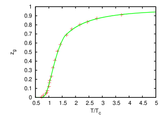
Figure 1: (Color online) Behavior of $z_{g}$ as a function of $T/T_{c}$. The points denote the values obtained from lattice data and solid line denote the fitting function. The fitting parameters are listed in Table. I.

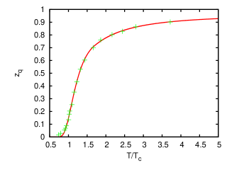
Figure 2: (Color online) Behavior of $z_{q}$ as a function of $T/T_{c}$. The points denote the values obtained from lattice data and solid line denote the fitting function. The fitting parameters are listed in Table. I.

For further analysis, we seek analytic forms for $z_{g}$ and $z_{q}$ as a function of temperature, which would render the computation more amenable. At this juncture, we note that there are limited number of lattice data for the pressure for a huge range of temperature ($(0.5-4.0)T_{c}$). Since the effective fugacities have been determined from the lattice pressure, the limitations get inherited by them as well, which further passed on to other thermodynamic quantities such as energy density, entropy density and trace anomaly. We hope that the functional form is not drastically altered by future refinements in lattice data.

We find that there is no universal functional form that describes the data in the full range of temperatures, either in the gluonic sector or the quark sector. There are some common features though. Both the sectors are characterized by a ’low temperature’ and a ’high temperature’ regime, with the cross over temperatures given by $x_{g,q}\equiv T_{g,q}/T_{c}\sim 1.68,1.70$ respectively. The functional forms on either side of $x_{g,q}$ are the same for both the sectors, but with different parameters. Thus, when $x<x_{q,g}$, the good fitting function has the form $a_{g,q}\ \exp(-b_{g,q}/x^{5})$. In the complimentary case $x>x_{q,g}$, it has the form $a^{\prime}_{g,q}\ \exp(-b^{\prime}_{g,q}/x^{2})$. The latter form is mandated by the fact that at high temperature the trace anomaly, $\frac{\epsilon-3P}{T^{4}}$ predominantly goes as $1/T^{2}$ cheng in lattice QCD. We list the fitting parameters for $z_{g}$ and $z_{q}$ in Table I.

Table 1: Fitting parameters for $z_{g}$ and $z_{q}$

$z_{g,q}$	$a_{g,q}$	$b_{g,q}$	$a^{\prime}_{g,q}$	$b^{\prime}_{g,q}$
Gluon	0.803$\pm$0.009	1.837$\pm$0.039	0.978$\pm$ 0.007	0.942$\pm$0.035
Quark	0.810$\pm$ 0.010	1.721$\pm$0.040	0.960 $\pm$ 0.007	0.846 $\pm$ 0.033

We shall utilize these forms to study temperature dependence of the trace anomaly in later part of the paper. We shall see that these forms correctly reproduce the high and low temperature behavior of the trace anomaly.

Temperature dependences of effective fugacities, in Fig. 1 and Fig. 2 reveal that the effective gluon and quark fugacities are of same order of magnitude for the whole range of temperature. This indicates that effective gluons and quarks contribute equally in our description. Its possible physical consequences, and an understanding from basic calculations in QCD is beyond the scope of the present work and will be a matter of future investigations.

It is worth noting that effective fugacity descriptions have been earlier employed in condensed matter systems in the last decade. To study the nature of Bose-Einstein (BE) condensation transition in interacting Bose gases, a parametric EOS in terms of the effective fugacity has been proposed by Li et. al li . This provides a scheme to explore the quantum-statistical nature of the BEC transition. There have been other works to study the non-interacting BE systems in harmonic trap 25 as well interacting bosonic systems 26 . Moreover, effective fugacity description has been used for a unitary fermion gas by Chen et al 24 for studying thermodynamics with non-Gaussian correlations.None of them employed the effective dispersion relations which we obtain naturally in this work. We shall now proceed to discuss the physical significance of the quasi-particle model and its viability.

III Physical significance and viability of the model

III.1 The modified dispersion relations

It has been emphasized in Ref. chandra2 that the physical significance of effective fugacity could be seen in terms of modified dispersion relations. The effective fugacities modify the single quasi-parton energy as follows,

$$\omega^{g}_{p} = p+T^{2}\partial_{T}ln(z_{g})$$

$$\omega^{q}_{p} = p+T^{2}\partial_{T}ln(z_{q})$$

$$\omega^{s}_{p} = \sqrt{p^{2}+m^{2}}+T^{2}\partial_{T}ln(z_{q}).$$ (8)

These dispersion relations can be interpreted as follows. The single quasi-parton energy not only depends upon the momentum but also gets contribution from the collective excitations of the quasi-partons. The second terms is like the gap in the energy due to the presence of quasi-particle excitations. This immediately reminds us of Landau’s theory of Fermi -liquids. Therefore, it is safe to say that the present quasi-particle model is in the spirit of Landau theory of Fermi liquids. These modified dispersion relations in Eq.(III.1) have emerged from the thermodynamic definition of the average energy of the system, due to the temperature dependent fugacities, $z_{g/q}$. Let us consider the expression for the energy-density, ${\epsilon}$ obtained in terms of the Grand Canonical partition function, ${\bf Z}$ as,

$$\epsilon=-\frac{1}{V}\frac{\partial\ln({\bf Z})}{\partial\beta}.$$ (9)

Substituting for the effective partition function (${\bf Z}=Z_{g}\times Z_{q}\times Z_{s}$), we obtain,

$$\epsilon \equiv\frac{\nu_{g}}{8\pi^{3}}\int d^{3}p\bigg{(}p+T^{2}\partial_{T}\ln(z_{g}))\bigg{)}f^{g}_{eq}$$ (10)

$$+\frac{1}{8\pi^{3}}\int d^{3}p\bigg{\{}\bigg{(}p+T^{2}\partial_{T}\ln(z_{q}))\bigg{)}\nu_{q}f^{q}_{eq}$$

$$+\bigg{(}\sqrt{p^{2}+m^{2}}+T^{2}\partial_{T}\ln(z_{q})\bigg{)}\nu_{s}f^{s}_{eq})\bigg{\}}$$

$$\equiv 3(P_{g}+P_{q}+P_{s})+\frac{T^{2}\partial_{T}\ln(z_{g})}{2\pi^{2}}\int d^{3}p\ \nu_{g}f^{g}_{eq}$$

$$+\frac{T^{2}\partial_{T}\ln(z_{q})}{2\pi^{2}}\int d^{3}p\ \bigg{(}\nu_{q}f^{q}_{eq}+\nu_{s}f^{s}_{eq}\bigg{)}.$$

The above equation can be recasted employing the expression for the pressure in terms of the temperature dependent, $z_{g/q}$ as,

$$\frac{(\epsilon-3P)}{T^{4}}=T\frac{\partial}{\partial T}\bigg{(}\frac{P}{T^{4}}\bigg{)}$$ (11)

Therefore, these modified dispersion relations naturally ensure the thermodynamic consistency condition in high temperature QCD, and lead to the trace anomaly, which we have discussed, in detail, in the next subsection. Moreover, these effective fugacities can be expressed in terms of effective quasi-particle number densities. These number densities leads to a simple Virial expansion for the EOS which we shall discuss in the next section.

Next, we look at the group velocity of quasi-partons. The group velocity can be obtained as $\vec{v}_{p}=\partial_{\vec{p}}\omega_{p}$. It is easy to see that the modified term in the dispersion relations is purely temperature dependent, therefore it will not change the group velocity of a quasi-parton. $\vec{v}_{p}=\hat{p}$ for quasi-gluons and quasi-quarks $(u,d)$ and $\vec{v}_{p}=\frac{\vec{p}}{\sqrt{p^{2}+m^{2}}}$. for strange quarks. The dispersion relation in Eq.(III.1) contributes to the trace anomaly in hot QCD which we shall discuss soon.

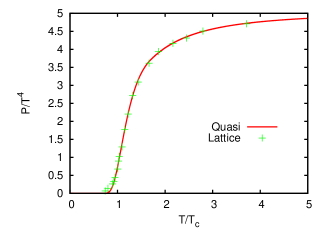
Figure 3: (Color online) Behavior of $P/T^{4}$ as a function of $T/T_{c}$. The quasi-particle pressure is obtained by using the fitting parameters for $z_{g}$ and $z_{q}$ listed in Table I. Lattice Data are also shown as points.

Let us now discuss the significance of of gluon condensate, in the hot QCD thermodynamics. In this context, D’Elia, Giacomo, and Meggiolaro ella have studied the electric and magnetic contributions to the condensate, and shown that near $T_{c}$ the former vanishes, however the latter remains unchanged. These authors investigated such effects by analyzing the two-point correlation functions both in pure-gauge sector, and the full QCD ella ; ella1 . It has been shown in casto that the effects of the gluon condensate are significant for $T\geq T_{c}$, and becomes vanishingly small beyond $2T_{c}$. Therefore, in the effective mass description of hot QCD for the temperatures, $T=1-2\ T_{c}$, one needs to consider the contributions of the condensate, while comparing the predictions on thermodynamic observables with the lattice QCD data. However, in our model, $z_{g}$, $z_{q}$ capture these effects, and we do not need to incorporate the contributions separately. This can be understood as follows, In the lattice data employed here, normalization of the pressure and energy density were chosen such that at $T=0$, these quantities vanish cheng , and the effects of the gluon condensate may be significant at higher temperatures. These effects are well captured in the trace anomaly in lattice QCD, which is the basic quantity computed in the lattice. And, all other thermodynamic quantities have been derived from the trace anomaly. In turn, these effects are automatically encoded in the pressure, the energy-density etc.. In our study, such effects have been captured in the effective fugacities, $z_{g/q}$ from the beginning, since, we have determined them from the lattice data on pressure. The gluon condensate contribute significantly to the energy density, entropy density, and the trace anomaly through the temperature derivatives of the $z_{g/q}$, in terms of modified dispersion relations.

Figure 4: (Color online) Behavior of $\epsilon/T^{4}$ as a function of $T/T_{c}$ in the quasi-particle model. The lattice results are shown as points and the solid line shows the quasi-particle result obtained by utilizing the fitting parameters, $a_{g,q},b_{g,q}$, and $a^{\prime}_{g,q},b^{\prime}_{g,q}$ listed in Table. I.

III.2 Viability of the model

As it has been already emphasized in the previous section that the model yields (2+1)-flavor lattice QCD EOS almost perfectly. To check further the viability of the model, we study the temperature dependence of the quasi-particle pressure,energy density, and the trace anomaly and check them against the direct lattice results. Lets us first discuss the temperature dependence of the pressure. We have plotted the quasi-particle pressure along with the lattice data in Fig. 3. We find that the agreement between the lattice data and quasi-particle model for the EOS is almost perfect beyond $T_{c}$. The temperature dependence of the energy density as a function of temperature is shown in Fig. 4. The quasi-particle results agree well with the lattice data beyond $T_{c}$.

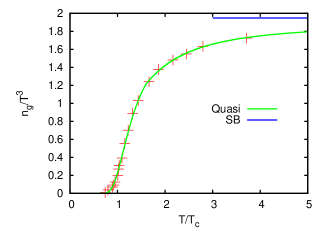
Figure 5: (Color online) Behavior of $n_{g}$ as a function of $T/T_{c}$. $N_{g}$ is obtained by employing the discrete data points for $z_{g}$ as well as fitting parameter for of $z_{g}$ listed in Table. I. The Stefan-Boltzmann (SB) limit of $n_{g}$ is also shown.

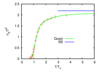
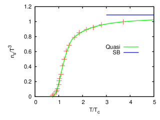
Figure 6: (Color online) Behavior of $n_{q}$ (left) and $n_{s}$ (right) as a function of $T/T_{c}$. They are obtained by employing the discrete data points for $z_{q}$ as well as fitting parameter for of $z_{q}$ listed in Table. I including the strange quark mass dependence. The Stefan-Boltzmann (SB) value is also shown beyond $3T_{c}$.

Encouraged from the crucial observation that lattice and quasi-particle model predictions are the same, we now proceed to study the trace anomaly as a function of temperature obtained from the quasi-particle model.

III.2.1 The trace anomaly

Trace anomaly gets contribution from all the three sectors. The gluonic and light quarks contributions come purely from the modified part of the dispersion relations. On the other hand, in the strange quark sector trace anomaly gets additional contribution from the mass. We denote the trace anomaly by $\Delta=(\epsilon-3P)\equiv\Delta_{g}+\Delta_{q}+\Delta_{s}$.

$$\frac{\Delta_{g}}{T^{4}} = T\partial_{T}\ln(z_{g})\frac{{n}_{g}}{T^{3}}$$

$$\frac{\Delta_{q}}{T^{4}} = T\partial_{T}\ln(z_{q})\frac{{n}_{q}}{T^{3}}$$

$$\frac{\Delta_{s}}{T^{4}} = T\partial_{T}\ln(z_{g})\frac{{n}_{s}}{T^{3}}$$

where $n_{g}$, $n_{q}$ and $n_{s}$ are the effective number densities for the quasi-partons and are defined by,

$${n}_{g} = \frac{\nu_{g}}{2\pi^{2}}\int^{\infty}_{0}dpp^{2}f^{g}_{eq}\equiv T^{3}\frac{\nu_{g}PolyLog[3,z_{g}]}{\pi^{2}}$$

$${n}_{q} = \frac{\nu_{q}}{2\pi^{2}}\int^{\infty}_{0}dpp^{2}f^{q}_{eq}\equiv T^{3}\frac{-\nu_{q}PolyLog[3,-z_{q}]}{\pi^{2}}$$

$${n}_{s} = \frac{\nu_{s}}{2\pi^{2}}\int^{\infty}_{0}dpp^{2}f^{s}_{eq}\equiv T^{3}\frac{-\nu_{s}PolyLog[3,-z_{q}]}{\pi^{2}}$$

$$-\frac{3\tilde{m}^{2}}{\pi^{2}}\ln(1+z_{q}).$$

We shall first discuss the behavior of these effective number densities as a function of temperature and thereby the temperature dependence of the trace anomaly in hot QCD. We determine the effective number densities exactly by the numerical evolutions of the integrals in Eq.(III.2.1). They are represented in terms PolyLog functions merely to understand the non-trivial temperature dependence of the effective number densities. Here, we see that $n_{g}/T^{3}$, and $n_{q/s}/T^{3}$ scales with $T/T_{c}$ in a non-trivial way. Their behaviors with temperature are shown in Figs. 5 and 6.

We have also shown the Stefan-Boltzmann value for the number densities in Figs. 5 and 6. $({n_{g}/T^{3}})|_{SB}=\nu_{g}\zeta(3)/\pi^{2}$; $({n_{q}/T^{3}})|_{SB}=3\nu_{q}\zeta(3)/{4\pi^{2}}$; and $({\nu_{s}/T^{3}})|_{SB}=3\nu_{s}\zeta(3)/{4\pi^{2}}$. Note that the SB limit has not been obtained even at $T=5T_{c}$. The effective number densities are roughly $\sim 10\%$ away at this temperature in all the three sectors. This is just the reflection of the fact that lattice EOS itself is away from SB limit there.

Using Table. I, the quantities $T\partial_{T}\ln(z_{g})$ and $T\partial\ln(z_{q})$ can easily be obtained as,

$$T\partial_{T}\ln(z_{g})=\left\{\begin{array}[]{rcl}\frac{5b_{g}}{x^{5}};&\mbox{x$\leq$ $x_{g}$}&\\ \frac{2b^{\prime}_{g}}{x^{2}};&\mbox{x$>$ $x_{g}$}&\end{array}\right.$$ (16)

$$T\partial_{T}\ln(z_{q})=\left\{\begin{array}[]{rcl}\frac{5b_{q}}{x^{5}};&\mbox{x$\leq$ $x_{q}$}&\\ \frac{2b^{\prime}_{q}}{x^{2}};&\mbox{x$>$ $x_{q}$}.&\end{array}\right.$$ (19)

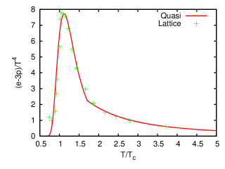
Figure 7: (Color online) Behavior of trace anomaly as a function of $T/T_{c}$. The solid line denotes the values obtained from the quasi-particle description and the points denotes the lattice results.

It is now straight forward to compute the trace anomaly employing the fitting functions for the effective fugacities; and effective quasi-particle number densities using Eq.(III.2.1). Behavior of $\Delta$ along with corresponding lattice values has been shown in Fig. 7. As it is clear from Fig. 3 and Fig. 7, pressure and trace anomaly computed by employing the quasi-particle model show good agreement with the lattice data of the same. This sets the utility of the model. Once these two quantities are known, it is straight forward to determine the energy density ($e$) and the entropy density($s$) by the standard thermodynamic relations, $e=3P_{quasi}+\Delta$, $s=\frac{e+P_{quasi}}{T}\equiv 4P_{quasi}+\Delta$.

If we see, closely the behavior of energy-density or the trace anomaly as a function of temperature in Figs. 4, and 7, we observe that around $T=1.7T_{c}$, both the quantities are not showing smooth behavior. There is no physical reason associated with this. This is merely the artifact of the two distinct fitting functions for $z_{g}$ and $z_{q}$ below and above this temperature. At this temperature these functions have different slopes. This problem may not be present, if we could have found a single fitting functions for $z_{g}$ and $z_{q}$ for the whole range of temperatures. As emphasized earlier, these fitting functions were needed to compute, the temperature derivatives of $z_{g}$ and $z_{q}$. Moreover, these points merely reflect the fact that at this point, perhaps various thermodynamic quantities are changing their slopes, but smoothly, which is not captured appropriately in the fitting functions. This may not be thought of as a serious problem since, one could compute the temperature derivatives of $z_{g}$ and $z_{q}$, directly by inverting relations in Eq. (12). In that case, we shall not get a continuous curve for energy density, rather discrete points and they will perfectly match with the lattice predictions.

IV Implications of the model

IV.1 Virial expansion for hot QCD

To translate QCD interactions in RHIC era in terms of a Virial expansion is quite a non-trivial task. There are very few attempts in this direction cassing . Here, we see that the quasi-particle understanding of equation of state for QGP plays very crucial role to obtain a very simple Virial expansion of the EOS in terms of effective quasi-particle number densities. The model tells us that the Virial expansion in (2+1)-flavor QCD could be subdivided in three sectors,viz., gluonic, light-quark, and strange quark sector and one can define the Virial expansion in each sector and finally combine them.

We begin with the purely gluonic sector first and subsequently discuss the matter sector (light quarks and strange quarks).

IV.1.1 Virial expansion in purely gluonic sector

To obtain the Virial expansion in this sector, we Taylor expand the pressure, $P_{g}$ and the effective gluon number density, ${n}_{g}$ in gluonic sector in the powers of $z_{g}$ (assuming $z_{g}<1$) and eliminate the explicit dependence of $z_{g}$ from both the expressions. This technique which is the standard way to obtain the Virial expansion of a ideal Bose/Fermi gas with fixed number of particles haung , is equally applicable here, although the systems are physically distinct, since $z_{g}$ and $z_{q}$ do not correspond to the particle conservation. The procedure is straight-forward. For the sake of completeness, we shall write a few steps. The expressions for $P_{g}$ and $n_{g}$ in the powers of $z_{g}$ are obtained as,

$$\frac{P_{g}}{\nu_{g}T}=\frac{1}{\lambda_{th}^{3}}\sum_{l=1}^{\infty}b_{l}\ z_{g}^{l}.$$ (20)

$$\frac{n_{g}}{\nu_{g}}=\frac{1}{\lambda_{th}^{3}}\sum_{l=1}^{\infty}l\ b_{l}\ z_{g}^{l}.$$ (21)

The quantity $\lambda_{th}\equiv{1/T}$ is the thermal wave length of gluons and the coefficient $b_{l}$ is given as,

$$b_{l}=\frac{1}{2\pi^{2}\ l}\int_{0}^{\infty}u^{2}\exp(-lu)du\equiv\frac{1}{\pi^{2}l^{4}}.$$ (22)

Consequently the ratio of Eq. (20) with Eq.(21) and expanding it as,

$$\frac{P_{g}}{{n}_{g}\ T}=\sum_{k=1}^{\infty}a_{k}(\tilde{N}_{g}\lambda_{th}^{3})^{k-1}\equiv\frac{\sum_{l=1}^{\infty}b_{l}\ z_{g}^{l}}{\sum_{l=1}^{\infty}l\ b_{l}\ z_{g}^{l}},$$ (23)

where $\tilde{N}_{g}=\frac{n_{g}}{\nu_{g}}$ and $a_{k}$’s are the Virial coefficients. Using, Eq. (20)and Eq.(21) in Eq.(23) and comparing the terms of order $z_{g}$, $z_{g}^{2}$ and $z_{g}^{3}$, we obtain,

$$a_{1} = 1;a_{2}=-\frac{b_{2}}{b_{1}^{2}}\equiv-\frac{\pi^{2}}{2^{4}};$$

$$a_{3} = \frac{\bigg{(}-2b_{3}+\frac{4b_{2}^{2}}{b_{1}}\bigg{)}}{b_{1}^{3}}$$

$$a_{4} = \frac{1}{b_{1}^{4}}\bigg{(}-3b_{4}-\frac{20b_{2}^{3}}{b_{1}^{2}}+\frac{18b_{2}b_{3}}{b_{1}}\bigg{)}.$$ (24)

One can, in principle obtain all the Virial coefficients comparing various order coefficients of $z_{g}$ in Eq.(23). Now, the Virial expansion up to $O((N^{\prime}_{g}\lambda_{th}^{3})^{3})$ can be written as,

$$\frac{P_{g}}{{n}_{g}\ T}=1+a_{2}(N^{\prime}_{g}\lambda_{th}^{3})+a_{3}(N^{\prime}_{g}\lambda_{th}^{3})^{2}+a_{4}(N^{\prime}_{g}\lambda_{th}^{3})^{3}.$$ (25)

If we exploit the temperature dependence of effective gluon number density shown in Fig. 5. We can compare the strength of various order terms in Eq.(25). We find that third term is $<<$ second term and fourth term is $<<$ third term. Remember that the Virial coefficients in Eq.(IV.1.1) do not acquire any temperature dependence and are same as those for an ideal gluonic plasma with temperature independent fugacity. The interactions merely renormalizes the number density of quasi-gluons. This confirms our view point that hot QCD medium effects can entirely be mapped in to the non-interacting/weakly interacting quasi-particle degrees of freedom. The validity of the Virial expansion in this sector is ensured by the fact that $N^{\prime}_{g}\lambda_{th}^{3}<<1$.

Let us now move to the matter sector and first discuss the light quark sector followed by the strange quark sector.

IV.1.2 Virial expansion in the matter sector

We shall exactly follow the same procedure discussed earlier to obtain the Virial expansion. We denote the light quarks contribution to pressure as $P_{q}$ and contribution from strange quarks to $P_{s}$. Expanding these quantities along with effective number densities ${n}_{q}$ and ${n}_{s}$ in the power of $z_{q}$ ( assuming $z_{q}<1$), we obtain the following expressions,

$$\frac{P_{q}}{\nu_{q}T} = \frac{1}{\lambda_{th}^{3}}\sum_{l=1}^{\infty}(-1)^{l-1}\ b_{l}\ z_{q}^{l}$$ (26)

$$\frac{P_{s}}{\nu_{s}T} = \frac{1}{\lambda_{th}^{3}}\sum_{l=1}^{\infty}(-1)^{l-1}\ b^{\prime}_{l}\ z_{q}^{l}$$ (27)

$$\frac{n_{q}}{\nu_{q}} = \frac{1}{\lambda_{th}^{3}}\sum_{l=1}^{\infty}(-1)^{l-1}l\ b_{l}\ z_{q}^{l}$$ (28)

$$\frac{n_{s}}{\nu_{s}} = \frac{1}{\lambda_{th}^{3}}\sum_{l=1}^{\infty}(-1)^{l-1}l\ b^{\prime}_{l}\ z_{q}^{l}.$$ (29)

Where the coefficients $b^{\prime}_{l}$ is defined as,

$$b^{\prime}_{l} = \frac{1}{2\pi^{2}\ l}\int_{0}^{\infty}u^{2}\exp(-l\sqrt{u^{2}+\tilde{m}^{2}})du$$ (30)

$$= b_{l}-\frac{\tilde{m}^{2}}{4\pi^{2}l^{3}}$$

Repeating the analysis same as for gluons, and denoting the Virial coefficients in light quark sector as $a^{q}_{l}$ and strange quark sector as $a^{s}_{l}$, the Virial expansion for $P_{q}$ and $P_{s}$ would have the following forms,

$$\frac{P_{q}}{n_{q}T}=a^{q}_{1}+a^{q}_{2}(N^{\prime}_{q}\lambda_{th}^{3})+a^{q}_{3}(N^{\prime}_{q}\lambda_{th}^{3})^{2}+a^{q}_{4}(N^{\prime}_{q}\lambda_{th}^{3})^{3}$$

$$\frac{P_{s}}{n_{s}T}=a^{s}_{1}+a^{s}_{2}(N^{\prime}_{s}\lambda_{th}^{3})+a^{s}_{3}(N^{\prime}_{s}\lambda_{th}^{3})^{2}+a^{s}_{4}(N^{\prime}_{s}\lambda_{th}^{3})^{3}.$$

where $N^{\prime}_{q}=\frac{n_{q}}{\nu_{q}}$ and $N^{\prime}_{s}=\frac{n_{s}}{\nu_{s}}$. In principle, all the Virial coefficients ($a^{q}_{l}$ and $a^{s}_{l}$) are possible to compute in terms of $b_{l}$ and $b^{\prime}_{l}$. We shall only discuss up to the fourth Virial coefficient. These coefficients are obtained as follows,

$$a^{q}_{1} = 1;\ a^{q}_{2}=\frac{b_{2}}{b_{1}^{2}}=\frac{\pi^{2}}{2^{4}};\ a^{q}_{3}=\frac{\bigg{(}-2b_{3}+\frac{4b_{2}^{2}}{b_{1}}\bigg{)}}{b_{1}^{3}}$$

$$a^{q}_{4} = \frac{1}{b_{1}^{4}}\bigg{(}3b_{4}+\frac{20b_{2}^{3}}{b_{1}^{2}}-\frac{18b_{2}b_{3}}{b_{1}}\bigg{)};$$

$$a^{s}_{1} = 1;\ a^{s}_{2}=(b_{2}-\frac{\tilde{m}^{2}}{2^{5}\pi^{2}})/(b_{1}-\frac{\tilde{m}^{2}}{2^{2}\pi^{2}})^{2};$$

$$a^{s}_{3} = \frac{\bigg{(}-2b^{\prime}_{3}+\frac{4({b^{\prime}_{2}})^{2}}{b^{\prime}_{1}}\bigg{)}}{({b^{\prime}_{1}})^{3}};$$

$$a^{s}_{4} = \frac{1}{({b^{\prime}_{1}})^{4}}\bigg{(}3b^{\prime}_{4}+\frac{20{(b^{\prime}_{2}})^{3}}{({b^{\prime}_{1}})^{2}}-\frac{18b^{\prime}_{2}b^{\prime}_{3}}{b^{\prime}_{1}}\bigg{)}.$$ (32)

Again the dominant contribution is from the second terms in the Virial expansion of $P_{q}$ and $P_{s}$ in Eq.(IV.1.2).This we have observed by exploiting the temperature dependence of the effective quasi-particle number densities shown in Fig. 6.

Since the total quasi-particle pressure is $P=P_{g}+P_{q}+P_{m}$, Virial expansion of the full EOS can be obtained by using the individual Virial expansions obtained in the effective gluonic sector (EGS), and the matter sector ( Eqs.(25) and (IV.1.2). Note that all the Virial coefficients in EGS as well as in the matter sector are independent of temperature. The information about the interaction has been captured in the effective quasi-parton number-densities. The second Virial coefficient is negative in the gluonic sector and positive in the quark sector. This is expected from the quantum statistics of quasi-gluons and quasi-quarks. It is straightforward an exercise to determine the other thermodynamic observables in term of effective quasi-parton number densities by using the well known thermodynamic relations. These expressions will also contain the temperature derivatives of effective number densities in addition. In other words, both $z_{g}$ and the modification factor to the dispersion relations, $T\partial_{T}\ln(z_{g})$, $T\partial_{T}\ln(z_{q})$ will appear in their expressions. Finally, the validity of the Virial expansion in the matter sector is ensured by the fact that $N^{\prime}_{q,s}\lambda_{th}^{3}<<1$.

This is perhaps the first time, we have obtained such a simple Virial expansion for hot QCD where interactions appear as suppression factors through the effective quasi-parton number densities. This has only been possible due to the quasi-particle description of hot QCD. Interesting enough, such a description works well down to temperatures which are of the order $1.0T_{c}$. The Virial expansion here highlights the role of interactions in hot QCD. The Virial expansion may possibly play crucial role to explore a quantitative understanding of Fermi liquid like picture of hot QCD interactions as indicated by our quasi-particle description and also play important role to develop effective field theory and effective kinetic theory for such a quasi-particle model. We shall leave these interesting issues for the future investigations.

At this juncture, we wish to mention that there has been a very recent attempt Virial to study the nuclear matter EOS at sub-nuclear density in a Virial expansion of a non-ideal gas. The Virial expansion is obtained by considering the fugacities for various species such as neutron, proton etc. The method to obtain the Virial coefficients is standard one as employed in the present work. However, the major difference between the two is in the physical meaning of the fugacities.

IV.2 Comparison with other approaches

We now intend to compare our quasi-particle model with other existing models. In the recent past 1 ; 2 ; 3 ; 4 and in a very recent work 5 , effects of hot QCD medium have been interpreted in terms of single particle states (effective gluons/quark-anti-quarks) via the Polyakov loop. In these approaches, the expectation value of the Polyakov loop appears in the effective gluon/quark-antiquark distribution functions 4 . It provides a suppression factor in the form of a effective fugacity to an isolated particle with color quantum numbers. On the other hand, there have been successful attempts to encode the high temperature QCD medium effects in terms of effective thermal masses for quasi-partons pesh ; peshier1 ; peshier2 ; alton ; alton1 . In the recent past, effective mass models have been employed to describe $(2+1)$-flavor QCD thaler ; kalman and the agreement was found to be good. The effective mass models, which we discussed so far are based on the lowest order results in perturbative QCD, equivalently leading order HTL results. These models are improved by incorporating the next order HTL contributions by Rebhan and Romatschle rebhan . Their predictions were shown to be in agreement with the lattice results including $(2+1)$-flavor QCD. Furthermore, there are other approaches which also involves quasi-particle picture of hot QCD along with the contribution from the gluon condensatecasto . We shall compare our model with these approaches one by one.

Let us consider the Polyakov loop approach first. There are certain similarities and a number of differences between our model and this approach. The similarities are, (i) both the approaches lead to an effective description of hot QCD in terms of free quasi-particles, (ii) the expectation value of the Polyakov loop which plays the role of effective fugacity as well as effective quasi-parton fugacities ($z_{g/q}$) in our model appear as the suppression factors in the corresponding quasi-parton distribution functions, (iii) in both the approaches the group velocity ($v_{gr}=\partial_{\vec{p}}\omega_{p}$), remains unchanged, (iv) both the models are quite successful in reproducing the lattice data on thermodynamic observables (For more details on Polyakov loop method see  3 . Our model yield lattice EOS for $SU(3)$ pure gauge theory almost perfectly which the deviations which are one part in a million chandra3 ), and same is true for the (2+1)-flavor lattice EOS, and (v) the effective gluon distribution function in 4 ; 5 has a similar mathematical structure as our model. In spite of these similarities, our model is fundamentally distinct from this approach. Our model is purely phenomenological, and is more in the spirit of Landau’s theory of Fermi liquids. We list below the major differences between the two approaches.

• The expectation value of the Polyakov loop appearing in the single particle distribution function does not change the dispersion relation for quasi-partons. On the other hand, in our model, we obtain non-trivial quasi-parton dispersion relations. $(T^{2}\partial_{T}ln(z_{g/q})$.

• The Polyakov loop (its phase) appears as an imaginary chemical potential in the single particle distribution functions 4 ; 5 . This is unlikely to happen in our model. The effective fugacities in our model cannot be interpreted as chemical potentials (real/imaginary) (since there is no conservation of particle number). They are introduced merely to capture all the interaction effects present in hot QCD medium.

• Employing our quasi-particle model, one can study the the bulk and transport properties of hot and dense matter (QGP) in RHIC. These studies have been reported for pure $SU(3)$ gauge theory in chandra3 ; chandra4 and will be presented separately for full lattice gauge theory in the near future.

Let us now compare our model with the effective mass models. In this approach, lattice QCD data for the EOS had been interpreted in terms of effective thermal gluon mass and effective thermal quark mass. The quasi-particle model proposed in this paper is completely distinct from this model. The major difference is in the philosophy itself. The effective fugacities are not the effective masses and they can be interpreted as effective mass in some limiting case ($p<<T^{2}\partial_{T}\ln(z_{g/q})$). Moreover, our approach explores the Fermi liquid like picture of hot QCD. Another major difference in two of the approaches can be realized in terms of group velocity $v_{gr}$, $v_{gr}$ in two approaches is not the same. In the effective mass approaches $v_{gr}$ depends on thermal mass parameter ($\vec{v}_{gr}=\vec{p}/\sqrt{p^{2}+m(T)^{2}}$). We have obtained a Virial expansion for hot QCD in terms of the the quasi-partons. This has not been done employing either of these two models.

Let us now discuss the quasi-particle models which incorporate the effects of gluon condensate explicitly in the analysis casto ; quasi_new2 . In these studies, the importance of the gluon condensate is highlighted, and its effect on the thermodynamic observables in hot QCD was studied in detail casto . In particular, Castorina and Mannarelli casto , have analyzed the thermodynamic properties of hot QCD between $1-2\ T_{c}$ by explicitly incorporating the gluon condensate along with the gluon, and quark quasi-particles with thermal masses. The results show excellent agreement with the lattice predictions, both in the pure glue sector and the full QCD sector. Apart from the differences in the dispersion relations, and the philosophy with our model, there has been a very crucial difference. As emphasized earlier, in our model the effect of gluon condensate has been incorporated from the beginning, and not treated explicitly as in casto . However, both the models are equally successful to describe the lattice QCD thermodynamics.

There is an alternate way to interpret the effective fugacities in terms of effective mass, as follows. Let us suppose, $z_{g/q}\equiv\exp(-m_{eff}|_{g/q}/T)$. The quantity, $m_{eff}$ can be thought of as $m_{eff}=g^{\prime}(T)T$, where $g^{\prime}$ is an effective coupling. It is to be observed that $z_{g/q}$ are of the order of $0.15$ around $T_{c}$; it leads to an estimate for $g^{\prime}\sim 2.0$. This indicates the non-perturbative nature of hot QCD matter near $T_{c}$. Moreover, $g^{\prime}$ becomes less than one beyond $1.3T_{c}$, and this observation is valid in both effective gluon and matter sector.

IV.3 Debye screening mass and charge renormalization

To investigate how the partonic charges modify in the presence of hot QCD medium, we consider the expression for the Debye mass derived in semi-classical transport theory manual in terms of equilibrium parton distribution functions. The same expression was obtained from the chromo-electric response functions of QGP chandra2 . The Debye mass in terms of the quasi-parton distribution functions, which are obtained from the (2+1)-lattice QCD EOS, is given by,

$$M^{2}_{D}=-2N_{c}Q^{2}\int\frac{d^{3}p}{8\pi^{3}}\partial_{p}f^{g}_{eq}+Q^{2}\int\frac{d^{3}p}{8\pi^{3}}\partial_{p}(4f^{q}_{eq}+2f^{s}_{eq}),$$ (33)

where $Q^{2}$ is the effective coupling which appears in the transport equation. If one assumes QGP as an ideal system of massless gluons and quarks, Eq.(33) reproduces the leading order HTL result for the Debye mass; with the identification that $Q^{2}\equiv g^{2}(T)$ ($g(T)$ is QCD running coupling constant at finite temperature).

Employing the distribution functions displayed in Eq.(II.1) to Eq. (33), we obtain the following expressions for the

$$M^{2}_{D} = Q^{2}T^{2}\bigg{(}\frac{N_{c}}{3}\frac{6\ Polylog[2,z_{g}]}{\pi^{2}}$$

$$+\frac{1}{2}\times\frac{-12\ PolyLog[2,-z_{q}]}{\pi^{2}}-\frac{\tilde{m}^{2}}{4\pi^{2}}\ln(1+z_{q})\bigg{)}.$$

While determining the Debye mass in Eq.(IV.3) from Eq.(33), we employ Eq.(II.1) and the following standard integrals,

$$\int_{0}^{\infty}p^{2}\ dp\frac{z_{g/q}\exp(-\beta p)}{(1\mp z_{g/q}\ \exp(-\beta p))^{2}} \equiv\pm\frac{2}{\beta^{3}}PolyLog[2,\pm z_{g/q}]$$

$$\int_{0}^{\infty}p\ dp\frac{z_{q}\exp(-\beta p)}{(1+z_{q}\ \exp(-\beta p))^{2}} \equiv\frac{1}{\beta^{3}}\ln(1+z_{q}).$$ (35)

The Debye mass with the Ideal EOS($z_{g}=1$, $z_{q}=1$) will be,

$$(M^{I}_{D})^{2}=Q^{2}T^{2}\bigg{(}\frac{N_{c}}{3}+\frac{1}{2}-\frac{\tilde{m}^{2}}{4\pi^{2}}\ln(2)\bigg{)}.$$ (36)

To analyze the role of interactions, we define the effective charges $Q_{g}$, $Q_{q}$, and $Q_{s}$ as,

$$Q_{g} = Q\ \bigg{\{}\bigg{(}\frac{6PolyLog[2,z_{g}]}{\pi^{2}}\bigg{)}^{1/2}\bigg{\}}$$

$$Q_{q} = Q\ \bigg{\{}\bigg{(}\frac{-12PolyLog[2,-z_{q}]}{\pi^{2}}\bigg{)}^{1/2}\bigg{\}}\equiv Q_{s}$$

Debye mass could be written in terms of these effective charges as,

$$M^{2}_{D}=\bigg{\{}\frac{N_{c}}{3}Q^{2}_{g}+\frac{1}{2}(Q^{2}_{q}+Q^{2}_{s})\bigg{\}}T^{2}-Q^{2}\ T^{2}\frac{\tilde{m}^{2}}{4\pi^{2}}\ln(1+z_{q}).$$ (38)

As stated earlier, in the ideal limit Eq.(38) will reduce to Eq.(36). The quantities, $Q_{g}$, and $Q_{q,s}$ approach to $Q$. This observation tells us that interactions merely renormalize the effective partonic charges. In fact, the effective charges are reduced as compared to $Q$ and asymptotically approach to the ideal value, $Q$.

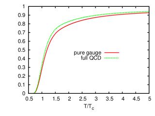
Figure 8: (Color online) Behavior of $\mu_{d}$ as a function of $T/T_{c}$. Note that $\mu_{d}$ approaches to the ideal value only asymptotically.

To see, how interactions modify Debye screening mass, we consider the ratio $\mu_{d}={M_{D}}/{M^{I}_{D}}$. The behavior of$\mu_{d}$ as a function of temperature is shown in Fig. 8. $\mu_{d}$ approaches the ideal value unity only asymptotically and $\mu_{d}\leq 1$. This implies that the presence of interactions suppresses the Debye mass as compared to its ideal counterpart.

Next, we compare $M_{D}$ with the Debye mass obtained in lattice QCD. Let us first discuss the Debye screening mass computed in lattice gauge theory. It has been calculated in pure gauge theory ($N_{f}=0$) kaz , in 2-flavor QCD ($N_{f}=2$) kaz1 ; ma1 , and in $2+1$-flavor QCD pet . The lattice data on Debye mass have been fitted with the simple ansatz motivated by leading order result on Debye mass, $m^{L}_{D}\equiv A\ m^{LO}_{D}$, where $m^{L}_{D}$ denotes the lattice data and, $m^{LO}_{D}\equiv\sqrt{(1+\frac{N_{f}}{6})}g(T)T$ denotes the leading order Debye mass. Here, $g(T)$ is the two loop running coupling constant. This form fits the data quite well if $A\approx 1.4-1.6$pet .

In our case (see Eq.38), $Q^{2}$ is a free parameter. We can fix it to match the Debye mass with the lattice result, $m^{L}_{D}$. This leads to,

$$Q^{2} = A^{2}\frac{g^{2}(T)}{(6\ PolyLog[2,z_{g}])/{\pi^{2}}},$$

$$Q^{2} = A^{2}\ g^{2}(T)\bigg{\{}\bigg{(}(6\ PolyLog[2,z_{g}]$$

$$-12\ PolyLog[2,-z_{q}])/{\pi^{2}}\bigg{)}-\frac{\tilde{m}^{2}}{4\pi^{2}}\ln(1+z_{q})\bigg{\}}^{-1}$$

in EGS and full QCD with $N_{f}$ flavors respectively. In other words, the Debye mass obtained from the quasi-particle model can exactly be matched with the lattice results for the Debye mass. The Debye mass is needed to determine the transport parameters for quark-gluon plasma in RHIC chandra3 . It is of interest to derive the form of heavy quark potential akhilesh ; chn_2 employing the formalism of chromo-electric response functions chandra2 ; akhilesh . While deriving the potential, one should keep in mind the fact that hadronic phase to quark-gluon plasma transition is a crossover crs1 ; crs2 rather than a true phase transition. These issues will be taken up in a separate communication in near future.

V Conclusions and future prospects

In conclusion, a quasi-particle model for $(2+1)$-flavor lattice QCD has been proposed which is valid in the deconfined phase of QCD. The interactions have been encoded in to the effective gluon and quark fugacities. These effective fugacities non-trivially modify the single quasi-parton energies and lead to the trace anomaly in hot QCD. The description accurately reproduce the lattice QCD pressure, energy-density, and the trace anomaly. In particular, the model accurately reproduce their low and high temperature behavior. We find that the model is fundamentally distinct from the other quasi-particle models (effective thermal mass, Polyakov loop models, and models with gluon condensate).

Employing the model, temperature dependence of the effective quasi-particle number densities has been obtained. A Virial expansion for QGP has been proposed in terms of effective quasi-particle number densities. The Virial expansion of the quasi-particle equation of state gets contribution from three sectors, viz., the effective gluonic sector, the light quark-sector, and the strange quark sector. These sectors were dealt separately and eventually lead to the complete Virial expansion. This is perhaps the first time such an Virial expansion has been proposed for hot QCD. Interestingly, the Virial expansions came out to be mathematically similar as that for an ideal system of gluons, light quarks and, strange quark with temperature dependent fugacities. The Virial expansion has ensured that the quasi-particle are non-interacting. The interactions merely modulate the quasi-particle number densities and modify the single quasi-particle energies in a non-trivial way.

The Virial expansion may play important role to explore the Fermi liquid like picture of hot QCD in the matter sector and, in building effective kinetic theory with the quasi-particle model. The Virial expansion has revealed that the interactions appear to various observables determined by employing the quasi-particle description only in two ways, either through the effective fugacities (act as modulation factors) or through the modified dispersion relation. Finally, Debye mass has been obtained employing the expression obtained from semi-classical transport theory and effective coupling has been determined in terms of effective fugacities. This observation will be required in determining the transport coefficients for quark-gluon plasma. We find the the Debye mass obtained from the quasi-particle model can exactly be matched with the lattice results.

The implications of model to study the transport coefficients (shear viscosity, bulk viscosity) will be taken up in the near future. It would also be of interest to extend the present model in the case of finite baryon density, and studying quark-number susceptibilities. It is to be of great interest to establish possible connections of our quasi-particle model with the Polyakov loop models, which is a matter of future investigations.

Acknowledgements: We are highly thankful to Prof. Saumen Datta for providing us the lattice data, and Prof. Rajeev Bhalerao for many helpful discussions and help in the computational part of the work. VC is thankful to Prof. Edward Shuryak for many helpful suggestions and encouragement. We are indebted to the people of India for their invaluable support for the research in basic sciences in the country.

References

- (1) Vinod Chandra, R. Kumar, V. Ravishankar, Phys. Rev. C 76, 054909 (2007).
- (2) Vinod Chandra, A. Ranjan, V. Ravishankar, Euro. Phys. J A 40, 109 (2009).
- (3) Vinod Chandra, V. Ravishankar, Euro. Phys. J C 64, 63 (2009).
- (4) STAR collaboration, J. Adams et al., Nucl. Phys. A 757, 102 (2005).
- (5) PHENIX Collaboration, Nucl. Phys. A 757, 184 (2005).
- (6) PHOBOS Collaboration , Nucl. Phys. A 757, 28 (2005).
- (7) BRAHMS Collaboration , Nucl. Phys. A 757, 1 (2005).
- (8) G. Boyd et al., Phys. Rev. Lett. 75, 4169 (1995); Nucl. Phys. B 469, 419 (1996).
- (9) F. Karsch, E. Laermann, A. Peikert, Phys. Lett. B 478, 447 (2000).
- (10) M. Cheng et al., Phys. Rev. D 77, 014511 (2008).
- (11) A. Bazavov et al., Phys. Rev. D 80, 014504 (2009).
- (12) M. Cheng et al, Phys.Rev. D 81,054504 (2010).
- (13) Szabolcs Borsanyi et al, JHEP 11, 077 (2010); Y. Aoki el al , JHEP 0601, 089 (2006); JHEP 0906, 088 (2009).
- (14) Szabolcs Borsanyi et. al, JHEP 1009 (2010) 073).
- (15) K. Aamodt et. al[The Alice Collaboration], arXiv:1011.3914 [nucl-ex].
- (16) K. Aamodt et. al [The Alice Collaboration], Phys. Rev. Lett. 105, 252301 (2010); Phys. Rev. Lett. 106, 032301 (2011).
- (17) T. Hirano, P. Huovinen, Y. Nara, arXiv:1012.3955[nucl-th].
- (18) X. -F. Chen, T. Hirano, E. Wang, X. -N. Wang, H. Zhang, arXiv:1102.5614[nucl-th].
- (19) R. Baier and P. Romatschke, arXiv:nucl-th/0610108.
- (20) H. B. Meyer, Phys. Rev. D 76, 10171 (2007)(arXiv:0704.1801(hep-lat)), A. Nakamura and Sunao Sakai, Phys. Rev. Lett. 94, 072305 (2005).
- (21) Lacey et. al, Phys. Rev. Lett. 98, 092301 (2007).
- (22) Zhe Xu and Carsten Greiner, Phys. Rev. Lett. 100, 172301; Zhe Xu, Carsten Greiner, Horst Stoecker, Phys. Rev. Lett. 101, 082302 (2008).
- (23) Adare et al, Phys. Rev. Lett. 98, 172301 (2007).
- (24) Sean Gavin and Mohamed Abdel-Aziz, Phys. Rev. Lett. 97, 162302 (2006).
- (25) M. Asakawa, S.A. Bass, B. Múller, Phys. Rev. Lett. 96, 252301 (2006); Prog. Theor. Phys. 116, 725 (2007).
- (26) Vinod Chandra, V. Ravishankar, Euro. Phys. J C 59, 705 (2009).
- (27) F. Karsch, D. Kharzeev, K. Tuchin Phys.Lett. B 663, 217 (2008) ; Dmitri Kharzeev, Kirill Tuchin, JHEP 09, 093 (2008).
- (28) Harvey B. Meyer, Phys. Rev. Lett. 100 162001, (2008).
- (29) Alex Buchel, Phys. Lett. B 663, 286 (2008).
- (30) P. Kovtun, D.T. Son, A. O. Starinets, Phys. Rev. Lett. 94, 111601 (2005).
- (31) E. V. Shuryak, Nucl. Phys. A 774, 387 (2006); hep-ph/0608177.
- (32) Kenneth G. Wilson, Phys.Rev. D 10, 2445 (1974).
- (33) Rajiv V. Gavai, Pramana 67, 885 (2006).
- (34) Frithjof Karsch, PoSCPOD07, 026 (2007) arXiv:0711.0656; PoSLAT 2007, 015 (2007) arXiv:0711.0661.
- (35) A. Peshier, B. Kampfer, G. Soff, Phys.Rev. C 61, 045203 (2000); Phys.Rev. D 66, 094003 (2002).
- (36) A. Peshier et. al, Phys.Lett. B 337, 235 (1994).
- (37) A. Peshier et. al, Phys. Rev. D 54, 2399 (1996).
- (38) C. R. Allton et. al, Phys. Rev. D 68, 014507 (2003).
- (39) C. R. Allton et. al, Phys.Rev. D 71, 054508 (2005).
- (40) A. Dumitru and R. D. Pisarski, Phys. Lett. B 525, 95 (2002).
- (41) K. Fukushima, Phys. Lett. B 591, 277 (2004).
- (42) S. K. Ghosh et al., Phys. Rev. D 73, 114007 (2006).
- (43) H. Abuki, K. Fukushima, Phys. Lett. B 676, 57 (2006).
- (44) H. M. Tsai, B Müller, J. Phys. G 36, 075101 (2009).
- (45) Vinod Chandra, V. Ravishankar, Nucl. Phys. A 848, 330 (2010).
- (46) Mingzhe Li, Haixiang Fu, Zhipeng Zhang and Jican Chen, Phys. Rev. A 75, 045602 (2007).
- (47) T. Haugerud, T. Haugset, F. Ravndal, arXiv:cond-mat/9605100.
- (48) Tor Haugset, Harek Haugerud and Jens O. Andersen, Phys. Rev. A 55, 2922 (1997); Jae Dong Noh, G. M. Shim and Hoyun Lee, Phys. Rev. Lett. 94, 198701 (2005); Klaus Kristen, David J. Toms, Physics Letters A 243, 137(1998).
- (49) Ji-sheng Chen, Jia-rong Li, Yan-ping Wang and Xiang-jun Xia, arXiv:0712.0205(cond-mat).
- (50) M. D’ Elia, A. Di Giacomo, E. Meggiolaro, Phys. Lett. B 408, 315 (1997).
- (51) M. D’ Elia, A. Di Giacomo, E. Meggiolaro, Phys. Rev. D 67, 114504 (2003).
- (52) P. Castorina, M. Mannarelli, Phys. Rev. C75, 054901 (2007); Phys. Lett. B 644, 336 (2007).
- (53) Statistical Mechanics, Kerson Haung, Pg. 219, Second edition, John Wiley & Sons.
- (54) S. Mattiello, W. Cassing,J. Phys. G 36, 125003 (2009); arXiv:0911.4647.
- (55) G. Shen, C. J. Horowitz, S. Teige, arXiv:1006.0489.
- (56) M. A. Thaler, R. A. Scheider, W. Weise, Phys. Rev. C 69, 035210 (2004).
- (57) K. K. Szabò, Anna I. Tòth, JHEP 06, 008 (2003).
- (58) A. Rebhan, P. Romatschke, Phys. Rev. D 68, 0250022 (2003).
- (59) Fabian Brau, Fabien Buisseret, Phys. Rev. D 79, 114007 (2009).
- (60) Kelly et. al, Phys. Rev. Lett. 72, 3461 (1994), Phys. Rev. D 50, 4209 (1995); Daniel F. Litim, C. Manual, Phys. Rep. 364, 451 (2002); J. P. Blaizot, E. Iancu, Phys. Rep. 359, 355 (2002).
- (61) O. Kaczmarek, F. Karsch, F. Zantow, and P. Petreczky, 2004 Phys. Rev. D 70, 074505 (2004); ibid 72, 059903 (2004).
- (62) O. Kaczmarek, F. Zantow, Phys. Rev. D 71, 114510 (2005).
- (63) Y. Maezawa et. al, Phys. Rev. D 75, 074501 (2007).
- (64) K. Petrov (RBC-Bielefeld Collaboration), PoS LAT 2007, 217 (2007).
- (65) A. Ranjan, V. Ravishankar, arXiv:0707.3697 [nucl-th].
- (66) Vinod Chandra, R. Kumar, V. Ravishankar, arXiv:0805.3199 [nucl-th]; V. Agotiya, Vinod Chandra, B. K. Patra, Phys. Rev. C 80, 025210 (2009).
- (67) Y. Aoki et. al, Nature 443, 675 (2006).
- (68) F. Karsch, hep-lat/0601013; Journal of Physics: Conference Series 46, 121 (2006).