Stepwise Filter Correlation Method and Evidence of Superposed Variability Components in GRB Prompt Emission Lightcurves

Abstract

Gamma-ray bursts (GRBs) have variable lightcurves. Although most models attribute the observed variability to one physical origin (e.g. central engine activity, clumpy circumburst medium, relativistic turbulence), some models invoke two physically distinct variability components. We develop a method, namely, the stepwise filter correlation (SFC) method, to decompose the variability components in a GRB lightcurve. Based on a low-pass filter technique, we progressively filter the high frequency signals from the lightcurve, and then perform a correlation analysis between each adjunct pair of filtered lightcurves. Our simulations suggest that if a mock lightcurve contains a “slow” variability component superposed on a rapidly varying time sequence, the correlation coefficient as a function of the filter frequency would display a prominent “dip” feature around the frequency of the slow component. Through simulations, we demonstrate that this method can identify significant clustering structures of a lightcurve in the frequency domain, and proved that it can catch superposed signals that are otherwise not easy to retrieve based on other methods (e.g. the power density spectrum analysis method). We apply this method to 266 BATSE bright GRBs. We find that the majority of the bursts have clear evidence of such a superposition effect. We perform a statistical analysis of the identified variability components, and discuss the implications for GRB physics.

1. Introduction

The temporal structure of Gamma-Ray Bursts (GRBs) exhibits diverse morphologies (Fishman & Meegan, 1995). They can vary from a single smooth pulse to extremely complex lightcurves with many erratic pulses with different durations, amplitudes, and fine structures. Based on temporal information, it has been difficult to categorize GRBs.

Physically, several mechanisms have been invoked to interpret GRB temporal variability. The leading scenario is to attribute the lightcurve variability to the irregularity of the central engine. For the commonly discussed internal shock scenario (Rees & Mészáros, 1994; Sari & Piran, 1997; Daigne & Mochkovitch, 2003; Maxham & Zhang, 2009), the observed time sequence tracks that of the central engine very well (Kobayashi et al., 1997; Maxham & Zhang, 2009). Alternatively, if the emission is from the central engine photosphere, then the observed lightcurve time history tracks that of the central engine directly (e.g. Lazzati et al., 2009). Within such a scenario, the observed lightcurves can be directly connected to the behavior of the central engine (e.g. Lei et al., 2007; Lu et al., 2008). A second scenario takes the opposite view: The observed variability originates in the emission region, which is not directly related to the history of central engine activity. Since the GRB outflow is relativistic, this requires that the emission region is not uniform. Rather, it contains locally Lorentz boosted emission regions, such as mini-jets (Lyutikov & Blandford, 2003) or relativistic turbulence (Narayan & Kumar, 2009; Kumar & Narayan, 2009). A third scenario discussed in the literature invoked a clumpy circumburst medium to interpret variability within the external shock model of GRB prompt emission (e.g. Dermer & Mitman, 1999). Swift observations of early X-ray afterglows of GRBs revealed a steep decay phase connected to the prompt emission lightcurve (Tagliaferri et al., 2005; Barthelmy et al., 2005). This suggests that the GRB prompt emission region is detached from the afterglow region, and therefore prompt emission should be of an “internal” origin (Zhang et al., 2006). This disfavors this third model of GRB variability.

Recently, Zhang & Yan (2011) proposed a new model of GRB prompt emission in the Poynting-flux-dominated regime, namely, the Internal-Collisioninduced MAgnetic Reconnection and Turbulence (ICMART) model. This model invokes a central engine powered, magnetically dominated outflow, which self-interacts and triggers fast magnetic turbulent reconnection to power the observed GRBs. An important prediction of the ICMART model is that it has two variability components: a broad (slow) component related to the central engine activity, and a narrow (fast) component associated with relativistic magnetic turbulence. Zhang & Yan (2011) conjectured that the visually apparent broad pulses in GRB lightcurves are related to the time history of the central engine (with each broad pulse corresponding to an ICMART event), while the much faster variabilities superposed on the broad pulses are related to relativistic, magnetic turbulence.

Alternatively, Morsony et al. (2010) simulated jet propagation from a massive star, and suggest that the broad pulses of several seconds duration are due to interaction of the jet with the progenitor, while the shorter scale variability in the millisecond range is related to that of the base of the inner engine (e.g. the black hole or the millisecond pulsar).

It would be essential to use rigorous mathematical methods to study GRB lightcurves to investigate whether the time sequence demands superposition of multiple variability components. Power density spectrum (PDS) is the most commonly used tool to study the temporal behavior of astronomical objects. Beloborodov et al. (1998, 2000) found that although the PDS of individual GRBs are diverse, the average PDS of a stack of GRBs is in accord with a power law with index -5/3 over 2 orders of magnitude in frequency. By locating the PDS peaks, Shen & Song (2003) revealed the typical variability time scales of some GRBs. In general, this method is not powerful to address whether a GRB lightcurve has superposed variability components. This is because it is insensitive to the lower frequency component (if it exists) since the GRB durations are typically not much longer than the broad pulses themselves. In the time domain, several methods have been developed to study temporal properties of GRBs. For example, lightcurves were decomposed into individual pulses using some parameterized empirical pulse functions (Norris et al., 1996) or a peak-finding algorithm (Li & Fenimore, 1996; McBreen et al., 2001; Nakar& Piran, 2002), and the temporal properties of the resulting pulses were analyzed. When performing the empirical pulse modeling, Norris et al. (1996) noted that some bursts are too complex to fit, possibly indicating pulse superposition. However, their matrix inversion algorithm failed to handle the problem. The peak finding selection method can decompose a lightcurve into many individual peaks. However, the method is not developed to reveal the superposed variability components.

Nonetheless, the possibility of superposition was suggested from other observational evidence. From a frequency-dependent analysis of prompt X-ray lightcurves of a sample of BeppoSAX GRBs, Vetere et al. (2006) discovered that the lightcurve tends to become smoother in softer energy bands. They then speculated that there might be a slow component superposed on a fast component. It is therefore of great interest to develop a rigorous mathematical method to identify such a superposition effect, if any, in gamma-ray lightcurves alone without the assistance of multi-wavelength data. Hereafter, we define a slow component as an underlying broad pulse component, while a fast component as the component of rapid variability that overlaps on top of the slow component.

In this paper, we develop a mathematical method to process GRB lightcurves as an effort of identifying the superpostion effect. This method, known as the stepwise filter correlation (SFC) method, is presented in detail in Section 2. We delineate its mathematical basis, and justify its robustness in identifying the superposed slow component through simulations. In Section 3, we apply this method to a sample of bright BATSE GRBs, and indeed identify the superposition effect in the majority of them. The properties of the identified slow components are studied statistically. The data analysis results and their physical implications are presented in Section 4. We note that some independent studies (e.g. R. Margutti et al. 2011, in preparation) reached the similar conclusion as ours.

2. Stepwise Filter Correlation Method

2.1. The method

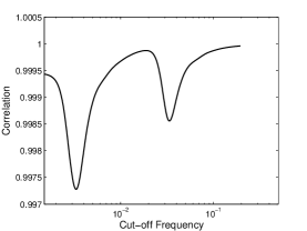
In signal processing, a filter is a device or process that removes some unwanted component or feature from a time sequence signal. Our method is based on a low-pass filter named Butterworth filter. For a certain cutoff frequency, this filter passes low-frequency signals below this frequency but attenuates signals above (see Appendix 1 for mathematical details). Our method is based on the following concept. Suppose that one specific time series (lightcurve) can be decomposed into the summation of $N$ pulses, either horizontally (pulses are laid out side by side) or vertically (superposition). One may denote the time scales (durations) of these pulses as $t_{\rm j,~{}j=1...N}$. The corresponding frequency for each pulse is therefore $f_{\rm j}=1/t_{\rm j}$. If one applies a stepwise filter in the frequency space, one would get a series of residual lightcurves (RLCs). If there is no pulse falling into the range between the cutoff frequencies $f_{\rm c,i}$ and $f_{\rm c,i+1}$, then the two RLCs should be identical. If there are some pulses whose frequencies fall into this range, the RLC with the lower cutoff frequency (RLC_i) should be smoother than the one with the higher cutoff frequency (RLC_i+1), since these pulses are screened after performing the low-pass filter at $f_{\rm c,i}$. The more pulses falling into this frequency range or the highger the amplitudes of these pulses, the more different the two RLCs look like. One can quantify the difference between the two RLCs using a statistical correlation method. A cluster of many pulses or a high amplitude of pulses within a frequency range would result in a correlation coefficient $R_{\rm i}$ (defined between RLC_i and RLC_i+1) to be more less than unity. By plotting $R_{\rm i}$ against $f_{\rm c,i}$, a “dip” in the curve would reveal such a clustering, and hence, would lead to the identification of a variability component around a particular frequency.

We realize such a concept based on the following procedure:

(1) For a time series, define a frequency range $(f_{\rm min},f_{\rm max})$ to be searched from. We then divide this frequency range into many discrete frequency bins uniformly in logarithmic scale. For all the GRBs, our frequency step is uniformly chosen as $\log(\Delta f)=0.05$. This gives a sequence of the cutoff frequencies $f_{\rm c,i}(i=1,...M)$, where $M$ is the total number of frequency bins. The low-pass filter to the original time series is then performed with each cutoff frequency $f_{\rm c,i}$ in turn. The RLC for each cutoff frequency, e.g. RLC_i corresponding to $f_{\rm c,i}$, is recorded.

(2) Perform a correlation analysis between each pair of adjunct RLCs (e.g. RLC_i vs. RLC_i+1). Record the Pearson’s correlation coefficient $R_{\rm i}$ for each pair.

(3) Plot $R_{\rm i}$ against $f_{\rm c,i}$, and identify apparent dips in the curve.

2.2. Simulation tests

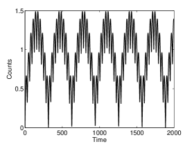
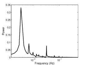
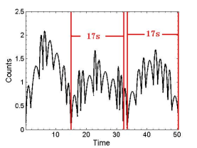
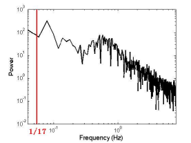
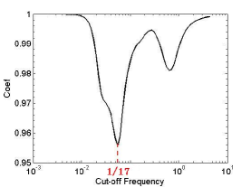
To prove the validity of the method, we perform some simulations. We start with a simple two-component lightcurve as shown in Fig.1 top row left panel. We superpose two periodic signals, both with the function form $A|\sin(\pi t/T)|$, where the periods of the two components are $T_{\rm s}=100\pi$ s for the slow component and $T_{\rm f}=10\pi$ s for the fast component, and the amplitude ratio between the two components is $A_{\rm s}:A_{\rm f}=2:1$. The middle panel of the top row shows the PDS of the lightcurve, which clearly shows the two components. The right panel of top row is the $R_{\rm i}-f_{\rm c,i}$ figure of our SFC method. Two dips that correspond to the two frequencies ($f_{\rm s}=1/100\pi~{}{\rm s^{-1}}$ and $f_{\rm f}=1/10\pi~{}{\rm s^{-1}}$ are clearly identified. We also add some white noise to the mock lightcurve. We find that even when the amplitude of the white noise is comparable to the signal, the dip in the lower frequency still shows up. This suggests that this method is powerful in identifying the low frequency component in the superposition.

Next, we simulate a more realistic lightcurve (middle row of Fig.1). The lightcurve (left panel of the middle row) is now a superposition of a slow component with pulse widths randomly distributed in the range of $T_{\rm s}=(10-20)$ s and a fast component with pulse widths randomly distributed in the range of $T_{\rm f}=(1-3)$ s. The amplitudes of the two components are randomly chosen in the range of $A_{\rm s}=(0.5-3)$ and $A_{\rm f}=(0.5-1)$, respectively. Since there is no strict periodicity and since the duration of the time series is not much longer than the slow component time scale, the PDS method (middle panel of the middle row) fails to identify the two frequency components. On the other hand, our SFC method (right panel of the middle row) clearly identifies a dip around 1/17 $s^{-1}$, which is right within the frequency range of the slow component. This simulation suggests that the SFC method is much more powerful in identifying the superposed components than the PDS method.

We note that the absolute value of the correlation coefficient $R$ depends on the step length of the cutoff frequency. A smaller frequency bin means smaller differences between consecutive RLCs, so that $R$ would be closer to 1. In any case, the global shape of the SFC $R_{\rm i}-f_{\rm c,i}$ curve (e.g. the location of the dips) does not depend on the size of the frequency bin, as long as it is small enough.

In order to further understand the SFC algorithm, we have performed a series of additional simulation tests (see Appendix 2 for details). These tests suggest that the SFC method is sensitive to significant clustering structures of a lightcurve in the frequency domain. A significant clustering structure is a cluster of frequencies that is separated from other frequency clusters, and that has a large enough amplitude. If a frequency cluster is too wide, or is too close to another frequency cluster, the corresponding dip is diminished. Similarly, if the amplitude of a frequency cluster component is too small, the corresponding dip would be too shallow or disappear completely. An interesting finding is that the quiescent gaps that separate pulses in GRB lightcurves (Ramirez-Ruiz et al., 2001) would complicate the analysis. Only when the gaps are removed manually, can one identify the corresponding frequencies of the slow pulse components (see Appendix 3 for details). Another finding is that if the slow component has only one pulse, the long tail of pulse tends to extend the duration, so that the identified duration can be much longer than the full width at half maximum (Appendix 2).

3. Application to GRB data

We now apply the SFC method to real GRBs. In this paper, our aim is to demonstrate the validity of the SFC method and to investigate whether the superposition effect exists in GRBs. So we do not pursue sample completeness. Rather, we only focus on some bright GRBs that have clear temporal structures.

We select 266 bright GRBs detected by Burst and Transient Source Experiment (BATSE) (Kaneko et al., 2006), whose lightcurve data and $T_{\rm 90}$ values are publically available from the online database http://heasarc.gsfc.nasa.gov/docs/cgro/batse/. In our analysis, we use light curves with 64 ms resolution obtained by BATSE in the four Large Area Detector energy channels, $20-300$ keV. The background is subtracted in each channel using linear fits to the 1024 ms data. The SFC method is then applied to these bursts. For all the analyses, we adopt a fixed maximum frequency of $f_{\rm max}=5$, which is based on the consideration of having at least 3 time bins for a 64 ms time resolution. The minimum frequency varies from burst to burst, but is related to a duration at least (sometimes larger than) $T_{90}$, in order to catch the slowest variability component. After fixing the frequency range, the frequency step is chosen evenly in the logarithmic space with $\log(\Delta f)=0.05$.

In order to quantitatively delineate the significance and confidence level of each dip, we define two parameters. The significance parameter, $s$, delineates the deepness/shallowness of a dip in the SFC $R_{\rm i}-f_{\rm c,i}$ curve. A dip is typically asymmetric, we apply the shallower wing of the dip to define its shallowness. We first identify the local minimum point at the bottom of the dip, e.g. for the $n$-th dip the coordinate ($f_{\rm n},R_{n}$) in the SFC curve. Next, we find out the inflection points (where the second derivatives change sign), or the turning points (where the first derivatives change sign) if an inflection point does not exist, in the left and right wings of the dip, respectively. These two points, i.e. ($f_{\rm n,left},R_{n,left}$) and ($f_{\rm n,right},R_{n,right}$), could be defined as “boundaries” of the dip. One can then define

$$S_{n}={\rm Min}\{\frac{R_{n,left}-R_{n}}{log(f_{\rm n})-log(f_{\rm n,left})},\frac{R_{n,right}-R_{n}}{log(f_{\rm n,right})-log(f_{\rm n})}\}$$ (1)

for each dip. A larger $S_{n}$ means a more significant dip. To reduce the bin-size effect, we normalize $S_{n}$ to the most significant one, $S_{n}^{\rm max}$ (which is usually the slowest one $S_{1}$), i.e. we define $s_{n}=S_{n}/S_{n}^{\rm max}$ for each dip. This $s$ parameter (which is $s\leq 1$) is then the significance parameter.

Next, we define a confidence level parameter, $c$, based on Monte-Carlo simulations. For each time bin with a particular observed count rate, we can generate a mock count rate based on the observed count rate $\mathcal{C}$ by randomly generating the data based on a normal distribution with ($\mathcal{C},\mathcal{\sqrt{C}}$). We then generate 1000 mock lightcurves by collecting these randomly generated count rates for each time bin. We apply the SFC method to each mock lightcurve, and identify the frequencies of the dips in each realization. For each dip in the original lightcurve, we define $c$ as the fraction that the simulations reproduce. We regard a component with high confidence level if $c\geq 0.9$, i.e., more than 900 simulations have revealed the component. We note that even though in general high-significance dips have a high confidence level, the two parameters are not always correlated. Some high “s” dips turn out to have a low “c”. We therefore evaluate both parameters for every dip measured in the SFC $R_{\rm i}-f_{\rm c,i}$ curves.

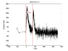
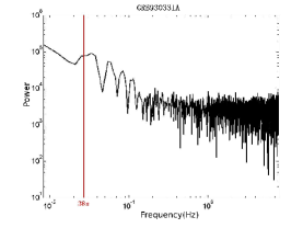
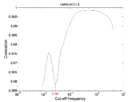
We take GRB 930331A as an example (bottom row of Fig.1). The left panel shows the original lightcurve, and the middle and right panels show the PDS and SFC analysis results, respectively. Although the PDS does not show any interesting feature, the SFC curve indeed shows a prominent dip around 1/38 ${\rm s^{-1}}$ (both significance and confidence level parameters equal unity, i.e. $s=1$, $c=1$). Checking back in the lightcurve, one indeed sees one broad pulse with a time scale of 38 s and another with the pulse width slightly shorter. Rapid spikes overlap on top of these two broad pulses. To verify whether the 38s component truly exists, we apply the SFC method to a portion of the lightcurve, from the trigger time $T_{\rm 0}$ to a certain time $T$, with $T$ stepwisely increasing in the range of $0<T-T_{0}<T_{90}$. We found that once $T-T_{0}$ is longer than 38s, the dip at 1/38$s^{-1}$ persists in all SFC curves, indicating that the 38s component is a real slow component.

Applying this method to our entire GRB sample, we find the following interesting facts.

(1) The total 266 bursts could be grouped into four categories based on both their lightcurves and SFC curves: (I) Good sample: 117/266 ($44.0\%$) of the bursts can be included in this sample. They clearly show at least one dip in the SFC curve. Checking back the lightcurves, one can usually find one or more pulses with the identified characteristic frequencies. Superposed on the identified slow component, there are always more rapid variability features. This clearly suggests a superposition of at least two variability components in the lightcurves. (II) Gap/long tail sample: 88/266($33.1\%$) of the bursts have quiescent periods in the lightcurve whose durations are comparable to the broad pulses, or have one FRED-like pulse with extended tail. For these cases, dips in the SFC curve are affected by the quiescent periods (gaps) and the tails. For the gap case, the real slow component can be revealed by manually removing the gaps in the lightcurves (see examples in Appendix 3). These bursts also clearly show the superposition effect as seen in the sample (I). However, since the identified frequencies do not well match the pulse durations, we have excluded these bursts in the statistical study presented below; (III) Irregular (noisy) sample: 24/266 ($9\%$) of the bursts show dips in the SFC curve. However, their lightcurves are too noisy to identify the corresponding components (see examples in Appendix 3). To be cautious, we do not include these bursts in the statistical analysis. (IV) Short/low temporal resolution sample: Finally, 37/266 ($13.9\%$) of the bursts are short bursts or long bursts whose lightcurves have a poor temporal resolution (see example in Appendix 3). These bursts have too narrow a frequency range to perform the SFC analysis. All the lightcurves and their corresponding SFC curves for the samples I-III are presented at the UNLV GRB group website http://grb.physics.unlv.edu/sfc. An example to each of the groups II, III and IV is presented in Appendix 3.

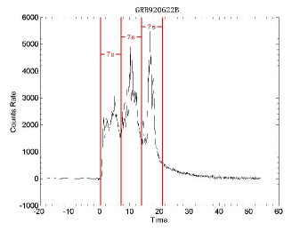
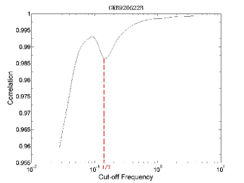
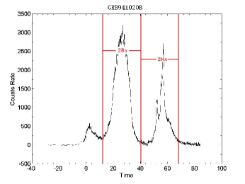
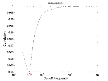
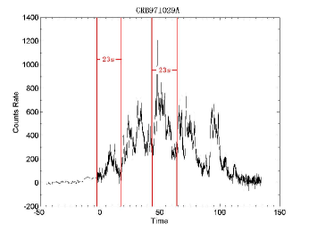
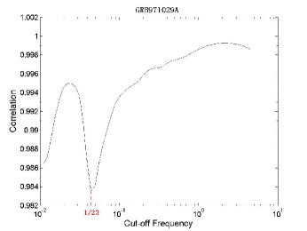
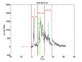
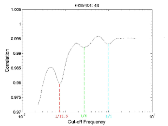
(2) Within Sample I (good sample), 30/117 ($25.6\%$) bursts show just one dip in the low frequency regime. Due to space limitation, we only present some examples in Fig.2. All the other cases are disseminated at the group website. The identified slow component time scales, as well as the $s$ and $c$ parameters for each dip are presented in Table 1. Since there is no strict periodicity in the lightcurves, the time scales of all the components we have identified are rough values, and we have rounded them to the nearest 0.5.

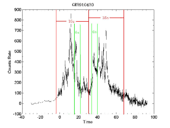
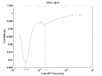
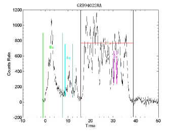
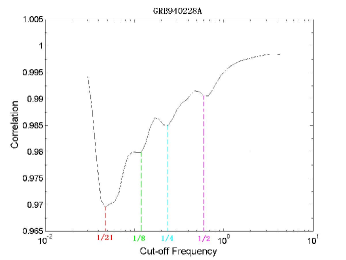
(3) The rest 87/117 bursts ($74.4\%$) in Sample I show more than one dips. For each dip we try to identify the corresponding component in the lightcurve. Some examples are presented in Fig.3. Others are presented in the group website. We present the time scales of all the identified components $T_{i}$ and their relevant $s$ and $c$ parameters also in Table 1, with increasing frequencies for ascending number $i$. Only dips with $c\geq 0.9$ are selected.

Inspecting the lightcurves with multiple dips in the SFC curve, we find that it is not always straightforward to relate dips with pulses in the lightcurves. In some cases (e.g. GRB 910430 and GRB 940414B), the low-frequency dip corresponds to a broad pulse with overlapping fast variability whose frequency corresponds to the high-frequency dips. In these cases, it is straightforward to identify the underlying broad pulses as the slow component, while to identify the overlapping narrow pulses as the fast component. In more complicated cases (e.g. GRB 940228A), besides identifying some slow components (e.g. 8s and 4s) that correspond to individual broad pulses, one also identifies a very slow (21s) component. This is due to clustering of multiple pulses to make a 21s “cluster”. In general, we caution that the SFC method, although sensitive to identify variability components not easy to unveil using the PDS method, may be over-sensitive to pick up variability components. We therefore caution that one should always go back to the lightcurves to clarify the physical nature of the frequency components identified in the SFC curves.

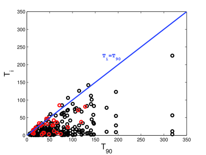
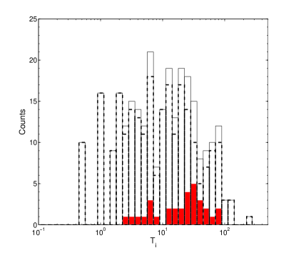
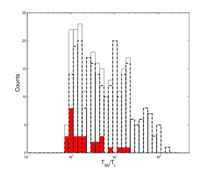
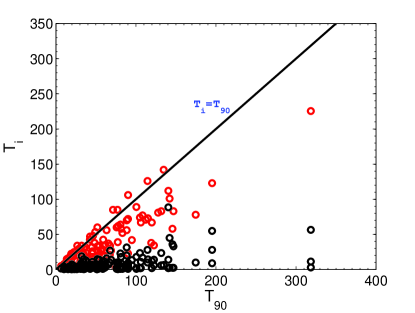
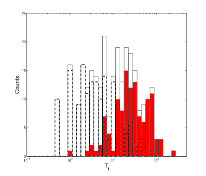
To understand the results better, we perform a statistical analysis on the time scales identified using the SFC technique. Figure 4 presents the identified variability timescales $T_{i}$ vs. the duration $T_{90}$ of the bursts, histogram of $T_{i}$, and histogram of $T_{90}/T_{i}$. First we focus on the one-dip only sample. The characteristic time scales $T_{1}$ of this sample are marked in red in Fig.4. The following trends can be observed: first, it seems that there is a very rough positive correlation between $T_{1}$ and $T_{90}$ (Fig.4a). This suggests that one tends to find longer slow components in longer bursts. Since there is a wide distribution in $T_{90}$, $T_{1}$ distributes from 2 s to 108 s (Fig.4b). On the other hand, the scatter of correlation is large. The ratio $T_{90}/T_{1}$ spans in at least one decade for this one-dip only sample. In some bursts, $T_{1}$ as small as $1/10$ of $T_{90}$ can be found (Fig.4c). Next, we include all the identified components ($T_{i}$) in the multi-dip sample (black circles in Fig.4a, and dashed histograms in Figs.4b and 4c). It is found that all the distributions are much wider. The overall histograms including all $T_{i}$ in the entire sample (solid histogram in Fig.4b and Fig.4c) cover 2 orders of magnitude in both $T_{i}$ and $T_{90}/T_{i}$. The spreading is mostly caused by the fast components identified in the multi-dip sample, but the long clusters (such as the 21s component identified in GRB 940228A) also contribute to the scatter. Since our frequency interval $\log\Delta f=0.05$ is uniform for all the bursts regardless of their $T_{90}$, our result does not suffer from the possible selection effect caused by different $T_{90}$. Inspecting the one-dip only sample, one usually also see the overlaping fast component, but with a lower amplitude than the multiple-dip ones. So these bursts are intrinsically similar to the multiple dip sample. The fast-component dips only show up when the high-frequency component amplitudes are large enough.

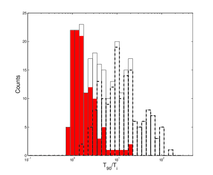
Another way to look at the distribution is to isolate the slowest component $T_{1}$ from other higher frequency ones. Figure 5 shows such a separation: $T_{1}$ in red and $T_{i}$ ($i>1$) in black. It can be seen that the $T_{i}-T_{90}$ correlation is more prominent for $T_{1}$. This may be because the longer the burst, the more probable that a long cluster (e.g. 21s cluster in GRB 940228A) would show up. The correlation between $T_{i}$ ($i>1$) is much weaker. In particular, variability time scales as short as seconds can appear in very long GRBs (e.g. $T_{90}\sim 250$ s). This suggests that the fastest variability component essentially does not depend on the duration of the burst.

4. Conclusions and Discussion

We have developed a new method (Stepwise Filter Correlation) to decompose variability components in a time series. Through Monte Carlo simulations, we demonstrate that this method can identify significant clustering structures of a lightcurve in the frequency domain, and is more powerful than the traditional methods (e.g. PDS) to identify superposed variability components, especially the slow variability component with duration comparable to the duration of the time series.

We then apply this method to GRB lightcurves as an effort to investigate whether the lightcurve is a superposition of multiple variability components. Our findings can be summarized as follows:

(1) We have applied this method to 266 BATSE bright GRBs, which may be grouped into 4 categories. In general, most bursts show a clear dip in the low frequency range, suggesting a slow component. By checking back to the lightcurves, we were able to identify the corresponding pulses with the relevant dip frequency in most of bursts. We found that such a slow component usually has superposed rapid variability components. We therefore conclude that GRB lightcurves are typically the superposition of multiple variability components.

(2) We selected 117 bursts as the good sample, and carried out a statistical statistical analysis sample. Among them, 30 show only one dip in the correlation curve. The other 87 GRBs have more than one dips. For the one-dip only sample in which the dip corresponds to a slow component, the distribution of this time scale $T_{1}$ spreads from several seconds to $\sim 100$s, with no typical time scales, and $T_{90}/T_{1}$ spreads in one order of magnitude (from $\sim 1$ to $\sim 10$). There is a rough trend of correlation between $T_{1}$ and $T_{90}$. Including all the variability components, the distributions of $T_{i}$ and $T_{90}/T_{i}$ spread in two orders of magnitude, without a characteristic value. The fastest time scale of order $\sim 1$s can be found in bursts with a wide range of durations.

The identification of the variability superposition effect (i.e. the existence of a slow component with overlapping faster variabilities) suggests that the causes of GRB lightcurve variabilities may be diverse. There might be more than one physical mechanisms that define the observed variability. This is in align with the prediction of the ICMART model (Zhang & Yan, 2011) and the jet propagation model (Morsony et al., 2010). The common aspect of these two suggestions is that the slow component (duration of seconds to 10s of seconds) is attributed to the engine that defines the jet variability. The difference between the two scenarios is the origin of the fast component. While the envelope model (Morsony et al., 2010) attributes it to the intrinsic variability at the base of the inner engine, i.e. the central black hole or magnetar, the ICMART model (Zhang & Yan, 2011) attributes it to relativistic magnetic turbulence in the emission region. These two scenarios may be further differentiated through testing more detailed predictions in both models. For example, in the jet-star interaction model, the inner engine powered variability shows up only if the input PDS is hard enough, e.g. $E(k)\propto k^{0}$, or essentially the same power per decade. It is not known whether this can be achieved in the inner engine, and such a hard PDS is not observed in the high frequency regime of GRBs. On the other hand, the fast variability in the ICMART model arises from locally Lorentz-boosted mini-jets due to relativistic turbulent reconnection. Simulations suggest that the it can reproduce the observed PDS (Zhang & Zhang, 2011). In any case, neither model predicts a characteristic time scale for the fast component. It is therefore still a theoretical challenge to account for the typical fast component time scales identified in some bursts.

Finally, we’d like to justify the Butterworth low-pass filter we have adopted. In principle, one can use low-pass, high-pass, or band-pass filters. First, a band-pass filter only passes signals in a certain frequency band, which is disfavored by the SFC method. This is because a good correlation between two adjacent frequency bins may simply reflect that the changes between the two frequency bins are similar. One may not get a “dip” even though the changes are significant. Second, the purpose of this work is to find out whether superposition exists in GRB lightcurves. We therefore care more about the underlying slow component. We therefore choose a low-pass filter, which is more sensitive to the slow component. A high-pass filter, on the other hand, would be more sensitive to fast components. As for specific digital low-pass filters, we have done simulation tests for several types, including the Butterworth filter, the Chebyshev filter, and the Gaussian filter. We find that different choices of filter would not change the results significantly. Among them, the Butterworth filter is designed to have as flat a frequency response as possible in the unscreened bandpass, which is beneficial to retain information of the slow component. We therefore adopt it in this work. We have also tried the wavelet transform method. It is a useful tool to unveil multiple variability components in the lightcurves (see e.g. Vetere et al. 2006). However, we did not find an easy way to quantify the results. We therefore do not apply the wavelet transform in this work.

Table 1Characteristic timescales identified in BATSE bright Gamma-Ray Bursts

GRB	$T_{\rm 90}$	$T_{\rm 1}$(s/c)	$T_{\rm 2}$(s/c)	$T_{\rm 3}$(s/c)	$T_{\rm 4}$(s/c)
910627	15.2	5 (1/1)	0	0	0
910807	59.6	12 (1/1)	0	0	0
911031A	90.0	23 (1/1)	0	0	0
911118A	19.2	22.5 (1/1)	0	0	0
920218C	122.5	55 (1/1)	0	0	0
920511A	48.5	3 (1/1)	0	0	0
920524	66.1	7.5 (1/1)	0	0	0
920622B	36.0	7 (1/1)	0	0	0
930331A	119.1	38 (1/1)	0	0	0
930425A	29.2	30 (1/1)	0	0	0
930916B	74.3	4 (1/1)	0	0	0
931106	152.1	108 (1/1)	0	0	0
931221A	57.9	29 (1/1)	0	0	0
940306	42.6	47 (1/1)	0	0	0
940520	32.8	2.5 (1/1)	0	0	0
940529D	37.6	42.5 (1/1)	0	0	0
941020B	56	28 (1/1)	0	0	0
950111B	46.3	48 (1/1)	0	0	0
950403A	14	12 (1/1)	0	0	0
950425	59.1	42.5 (1/1)	0	0	0
951202	28.5	34 (1/1)	0	0	0
960114	36.5	32.5 (1/1)	0	0	0
960807	12.7	6 (1/1)	0	0	0
961102	71.4	85 (1/1)	0	0	0
970202	26.7	34 (1/1)	0	0	0
970223	16.3	16 (1/1)	0	0	0
970807B	37.6	7 (1/1)	0	0	0
970912B	65.6	37 (1/1)	0	0	0
971029A	89.9	23 (1/1)	0	0	0
971220A	13.6	15 (1/1)	0	0	0
980124A	45.1	32 (1/1)	0	0	0
980225	127.7	81 (1/1)	0	0	0
980329A	18.5	20 (1/1)	0	0	0
991121	112.2	71 (1/1)	0	0	0
000302A	22.7	28.5 (1/1)	0	0	0
910425	90.2	106 (1/1)	9.5 (0.65/1)	4 (0.41/1)	0
910430	62.0	35 (1/1)	6 (0.11/1)	0	0
910601	28.5	20 (1/1)	4.5 (0.36/1)	0	0
910614	146.9	83 (0.65/1)	33 (1/1)	2.5 (0.02/0.98)	0
910619	106.1	67 (1/1)	11 (0.06/1)	2 (0.05/1)	0
910814A	77.8	62 (1/1)	10 (0.3/1)	0	0
910905	81.5	58 (1/1)	18 (0.64/0.96)	9 (0.77/1)	0
911127A	18.8	18 (1/1)	2 (0.046/1)	0	0
911202A	20.1	22 (1/1)	7 (0.2/0.99)	0	0
920110A	318.6	225.5 (1/1)	56.5 (0.33/1)	11.5 (0.1/1)	3 (0.027/1)
920210B	51.8	60 (1/1)	15 (0.25/0.97)	0	0
920308A	51.1	11 (1/1)	5 (0.53/1)	1 (0.15/1)	0.5 (0.03/0.99)
920513	88.6	70 (1/1)	4 (0.74/1)	2 (0.42/1)	0
920525B	16.1	8 (1/1)	4 (0.67/1)	0	0
920617B	67.7	34 (0.03/1)	27 (1/1)	0	0
920627B	52.8	26.5 (1/1)	4 (0.11/1)	3 (0.1/1)	1 (0.17/1)
921015	272.4	108 (0.6/1)	48 (1/1)	0	0
921118	174.7	78 (1/1)	10 (0.18/1)	0	0
921206B	53.8	21 (1/1)	3 (0.46/1)	0	0
921209B	38.1	9.5 (1/1)	3 (0.76/1)	0	0
921230A	18.8	16 (1/1)	2 (0.17/0.9)	0	0
930309A	90.1	72 (0.83/1)	7 (1/1)	1 (0.8/1)	0
930506B	22.1	22 (1/1)	5.5 (0.03/1)	2 (0.15/1)	0
930720A	45.9	26 (0.7/1)	5 (0.5/1)	2.5 (1/1)	0
930910C	83.1	52 (1/1)	4 (0.03/1)	3 (0.07/1)	1 (0.11/1)
931026	134.7	142 (1/1)	6.5 (0.04/1)	0	0
940128B	45.2	18 (1/1)	7 (0.2/1)	0	0
940210	30.7	12 (1/1)	1.5 (0.16/1)	1 (0.28/1)	0
940228A	33.3	21 (0.3/1)	8 (1/0.93)	4 (0.65/1)	2 (0.4/1)
940301	42.5	42.5 (1/1)	2 (0.05/1)	0	0
940302	119.9	67 (0.82/1)	12 (0.59/1)	2 (0.21/1)	0
940319	75.9	60 (1/1)	10 (0.3/1)	2.5 (0.08/1)	1 (0.11/1)
910321	51.6	16 (1/1)	3 (0.2/1)	0.5 (0.15/1)	0
940323	60.7	6 (1/1)	2.5 (0.19/1)	0	0
940414B	42.8	13.5 (1/1)	4 (0.2/1)	1 (0.16/1)	0
940619	88.4	56 (0.34/1)	31.5 (0.67/1)	20 (1/0.98)	5 (0.35/1)
940703A	34.9	30 (1/1)	15 (0.4/1)	3.5 (0.12/1)	0.5 (0.03/1)
940806D	10.2	3.5 (0.5/1)	0.5 (1/1)	0	0
940817	32.2	34 (0.62/1)	19 (1/1)	8.5 (0.5/1)	2.5 (0.7/1)

Table 1Continued

GRB	$T_{\rm 90}$	$T_{\rm 1}$(s/c)	$T_{\rm 2}$(s/c)	$T_{\rm 3}$(s/c)	$T_{\rm 4}$(s/c)
941014A	45.4	23 (1/1)	11 (0.65/1)	6 (0.15/1)	4 (0.25/1)
941017A	77.1	85 (1/1)	7 (0.05/1)	4 (0.03/1)	1.5 (0.09/1)
941023A	34.9	22 (1/1)	11 (0.2/1)	5.5 (0.34/1)	0
941119	33.4	24 (1/1)	5 (0.06/1)	2.5 (0.09/1)	0
941126E	36.1	13 (1/1)	1 (0.03/0.99)	0	0
950208	58.6	18.5 (1/1)	7 (0.24/1)	1 (0.21/1)	0
950211B	54.3	34 (0.43/1)	14 (1/1)	3 (0.43/1)	0
950608	142.0	101 (0.77/1)	45 (1/1)	2.5 (0.15/0.97)	0
950701B	10.6	7 (0.95/1)	4 (1/1)	0	0
950706	68.9	27 (1/1)	14 (0.38/1)	0	0
950909	65.7	21 (1/1)	7 (0.2/1)	0	0
951011	31.5	28 (1/1)	4 (0.55/1)	2.5 (0.75/0.98)	0
951219	58.8	21 (1/1)	4 (0.8/1)	1.5 (0.15/1)	0
960322A	22.8	25 (1/1)	2.5 (0.14/1)	0	0
960524C	80.6	64 (0.84/1)	23 (1/1)	3.5 (0.28/0.93)	1 (0.3/1)
960607B	140.5	112 (0.11/1)	88.5 (1/1)	14 (0.69/1)	2 (0.11/0.91)
960824	229.9	82 (1/1)	6.5 (0.05/1)	2.5 (0.07/0.9)	0
961228C	60.0	34 (0.54/1)	12 (0.4/1)	4 (1/1)	0
970111	31.5	13 (0.07/1)	9 (1/1)	0	0
970306	122.5	34.5 (0.52/1)	14 (0.18/1)	6 (1/1)	0
970315B	16.8	6.5 (0.98/1)	3.5 (0.1/1)	2 (1/1)	1 (0.76/1)
970411	58.9	53.5 (1/1)	3.5 (0.06/1)	0	0
970420	10.5	8 (1/1)	2 (0.81/1)	1 (0.5/1)	0
970612B	37.6	24 (0.07/1)	13 (1/1)	2.5 (0.4/1)	0
970816	6.5	5 (1/1)	1.5 (0.36/1)	0	0
970831	114.5	126 (1/1)	28 (0.34/0.94)	10 (0.11/1)	0
971110	195.2	123 (1/1)	55 (0.21/1)	28 (0.95/1)	9 (0.53/1)
971207C	48.3	38 (0.74/1)	5.5 (1/1)	0	0
980105	36.8	10 (0.42/1)	6.5 (1/1)	1 (0.24/1)	0
980203B	23.0	6 (1/1)	2 (0.42/1)	1.5 (0.9/1)	0.5 (0.42/1)
980208B	31.2	12 (1/1)	6.5 (0.42/0.96)	1.5 (0.16/1)	0
980315B	105.0	74 (0.93/1)	23.5 (1/1)	2 (0.13/0.96)	0
980703B	108.4	77 (1/1)	17 (0.25/1)	0	0
980803	19.8	21 (0.03/1)	7.5 (1/1)	1.5 (0.1/1)	0.5 (0.29/1)
980923	33.0	15 (1/1)	5 (0.44/1)	2 (0.39/1)	1 (0.15/1)
990108	145.7	58 (0.04/0.98)	36 (1/1)	3 (0.05/0.99)	0
990111A	15.0	14 (1/1)	1.5 (0.12/1)	0	0
990123A	63.4	56 (1/1)	16 (0.74/1)	0	0
990316B	100.5	89 (1/1)	18 (0.14/1)	2 (0.05/1)	1 (0.05/1)
990323C	49.5	17.5 (1/1)	5 (0.18/1)	2 (0.46/1)	0
990728	42.8	15 (1/1)	3 (0.39/1)	0	0
990803	19.4	1 (1/1)	0.5 (0.45/0.99)	0	0
991004D	77.4	39 (0.69/1)	9.5 (1/1)	0.5 (0.22/1)	0
991009	131.6	83 (1/1)	23.5 (0.29/1)	6 (0.11/1)	0
991113	61.4	13 (1/1)	3 (0.76/1)	0	0
991127	52.7	8 (1/1)	1.5 (0.39/1)	0	0
991216	15.2	16 (1/1)	3 (0.55/1)	1 (0.11/1)	0.5 (0.1/1)
000101	51.8	33 (0.8/1)	7 (1/1)	0	0
000103	67.4	21 (0.79/1)	10 (1/1)	0	0
000201A	95.0	42 (1/1)	13.5 (0.19/1)	6 (0.08/1)	0
000221	26.2	12 (1/1)	0.5 (0.05/1)	0	0
000511A	115.0	73 (1/1)	14.5 (0.1/1)	0	0

Figure 1.— Examples that prove the validity of the SFC method. Top panel: The first simulation test; Middle panel: the second simulation test; Lower panel: a real GRB 930331A). In all three panels, the left figure is the simulated or real lightcurve, the middle figure is power density spectrum, and the right figure is the correlation curve, i.e. the correlation coefficient $R_{i}$ versus the cutoff frequency $f_{\rm c,i}$.

Figure 2.— Examples for the one-dip only bursts. The left panel are the lightcurves, and the right panel are the correlation curves. The pulses that correspond to the identified frequencies are marked in the lightcurves. The time scales are rounded to the nearest 0.5.

Figure 3.— Examples for the multi-dip bursts. The left panel are the lightcurves, and the right panel are the correlation curves. The pulses that correspond to the identified frequencies are marked in different colors in the lightcurves. The time scales are rounded to the nearest 0.5.

Figure 4.— Statistical results of the identified characteristic frequencies. (a) The $T_{i}-T_{90}$ distribution; (b) histogram of $T_{i}$; and (c) histogram of $T_{90}/T_{i}$. The time scales identified in the one-dip sample are marked in red. In (a) the black circles denote the time scales identified in multi-dip GRBs. In (b) and (c), the dashed histograms are for the multi-dip sample, and the final solid histograms are for the entire sample.

Figure 5.— The same as Fig.4, except the red color denotes the slowest time scale in all bursts, and black denotes the rest.

Appendix A 1. Butterworth Low-pass Filter

For a time series signal $S(t)$ passing an ideal low-pass filter with cutoff angular frequency $\omega_{c}=2\pi f_{c}$, the residual signal would read (Oppenheim et al., 1998)

$$S(\tau,\omega_{c})=\frac{1}{\pi}\int_{-\infty}^{\infty}{\frac{S(t)\sin[\omega_{c}(\tau-t)]}{\tau-t}}dt.$$ (A1)

For example, if $S(t)=\sin(At)$, then one has

$$S(\tau,\omega_{c})=\frac{\sin(A\tau)}{2}\times[{\rm Sign}(1-\frac{A}{\omega_{c}})+{\rm Sign}(1+\frac{A}{\omega_{c}})]~{},$$ (A2)

where “Sign” is the sign symbol of the expression. This formula can be translated to

$$S(\tau,\omega_{c})=\left\{\begin{array}[]{ll}0,&\mbox{$\omega_{c}<A$}\\ \frac{\sin(A\tau)}{2},&\mbox{$\omega_{c}=A$}\\ \sin(A\tau),&\mbox{$\omega_{c}>A$}\end{array}\right.\$$ (A6)

which shows that the high-frequency signal is attenuated.

For a signal as the sum of two periodic components, e.g., $S(t)=\sin(At)+\sin(Bt)$ with $A<B$, one can derive

$$S(\tau,\omega_{c})=\left\{\begin{array}[]{ll}0,&\mbox{$\omega_{c}<A$}\\ \frac{\sin(A\tau)}{2},&\mbox{$\omega_{c}=A$}\\ \sin(A\tau),&\mbox{$A<\omega_{c}<B$}\\ \sin(A\tau)+\frac{\sin(B\tau)}{2},&\mbox{$\omega_{c}=B$}\\ \sin(A\tau)+\sin{B\tau},&\mbox{$\omega_{c}>B$}\end{array}\right.\$$ (A12)

It is obvious to see how the two signals are screened when a progressively lower angular cutoff frequency is applied. If one chooses two angular cutoff frequencies that satisfy $\omega_{\rm c,i}-\omega_{\rm c,i-1}<B-A$, one would get a correlation coefficient between two RLCs to be $R_{\rm i}=1$ if $A\&B\nsubseteq(\omega_{c,i}\sim\omega_{c,i-1})$, or $R_{\rm i}\ll 1$ if $A|B\subseteqq(\omega_{c,i}\sim\omega_{c,i-1})$.

Similar results can be obtained if one sets $S(t)=\cos(At)$ or $S(t)=\cos(At)+\cos(Bt)$ with $A<B$.

For a more complicated time series, one can always decompose it into the summation of many $Sine$ or $Cosine$ functions through Fourier transforms. For any angular cutoff frequency $\omega_{\rm c,i}$ (and the corresponding cutoff frequency $f_{\rm c,i}=\omega_{\rm c,i}/2\pi$), the low-pass filter then attenuates the signal above this frequency.

Appendix B 2. Additional simulation tests of the SFC algorithm

In order to better understand the SFC algorithm, we perform a set of additional simulations.

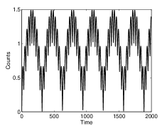
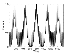
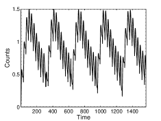
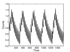
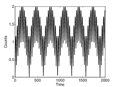
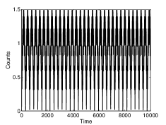
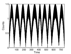
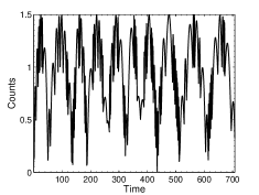
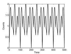
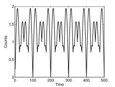
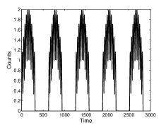
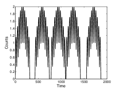
1) Pulse profiles: We test four different pulse profile functions, $A|\sin(\pi t/T)|$ (sine) function, Gaussian function, and two “FRED” profiles proposed by Kocevski et al. (2003) and Norris et al. (1996). First, we generate multiple pulses lying side-by-side with a fast component superposed on the slow component. For all four different pulse functions, the pulse durations of the slow and fast components are fixed to $100\pi$ and $10\pi$, respectively, with the amplitude ratio between the two components fixed as $A_{\rm s}:A_{\rm f}=2:1$. As shown in Fig.6(a-h), we can see that SFC is not sensitive to the pulse profile function in the multi-pulse case. In the rest of the simulation tests invoking multi-pulse lightcurves, we adopt the sine function as examples, and use Fig.6(a,b) as our nominal test to be compared with others (see tests 2-6 below). Since the SFC method can catch a frequency component even if only one pulse exists (test 3 below) and since some GRBs indeed only have one broad pulse, next we test the four pulse profile functions for one pulse only. We fix the full width at half maximum (FWHM) to $\sim 200$ s, and vary the function shapes. To our surprise, it is found that the identified typical durations from the SFC curve dip frequencies are very different for the four functions (Fig.6(i-p)): $\sim 470$ s for the sine shape, $\sim 500$ for the Gaussian shape, $\sim 676$ s for the Norris’ shape, and $\sim 708$ s for the Kocevski’s shape. A closer investigation suggests that the longer durations for the FRED shapes are mostly due to the extended tails for these profile functions (Norris et al., 1996; Kocevski et al., 2003). This explains the identified long durations for some FRED-like lightcurves in Sample II (gaps and long tails), which can be longer than $T_{90}$ in some cases.

2) Amplitude of pulses: The amplitude of a frequency components is an important factor. For our superposition tests, the relative depths of the dips depend on the amplitude ratio of the slow and fast components. This can be seen from the comparison of Fig.6(a,b) for $A_{\rm s}:A_{\rm f}=2:1$ and Fig.7(a,b) for $A_{\rm s}:A_{\rm f}=1:1$ (with the nominal parameters $T_{s}=100\pi$ s, and $T_{f}=10\pi$ s). For this set of parameters, the fast component dip disappears when $A_{\rm s}:A_{\rm f}>15:1$, while the slow component dip disappears when $A_{\rm s}:A_{\rm f}<1:25$. The asymmetry is understandable since a low pass filter favors the slow component.

3) Number of pulses: Fixing the nominal parameters but increasing the number of pulses, we find that the corresponding dips in the SFC $R_{\rm i}-f_{\rm c,i}$ curve become deeper. See Fig.7(c,d) as compared with Fig.6(a,b). On the other hand, the slow component can be detected even with one single broad pulse, as long as its amplitude is large enough. See Fig.6(i-p).

4) Pulse duration spread: Similar to the mock light curve shown in the middle panel of Fig.1, we generate a set of light curves whose slow component duration range is fixed in $T_{\rm s}=(50-100)$ s and the amplitude ratio is fixed to $A_{\rm s}:A_{\rm f}=2:1$. We gradually spread the fast component duration range. We find that the significance of the relevant dip of the fast component in the SFC $R_{\rm i}-f_{\rm c,i}$ curve diminishes and eventually disappears as the frequency spread is wide enough (Fig.7(e-h)).

5) Separation between two components: Back to the two-frequency case, we fix the amplitude ratio as $A_{\rm s}:A_{\rm f}=1:1$ and the slow component duration as $T_{\rm s}=100$, and then gradually brings the fast component duration closer and closer to the slow one. We find that the significance of the relevant dip of fast component in the SFC $R_{\rm i}-f_{\rm c,i}$ curve diminishes, and merges with the slow frequency component when $\frac{f_{\rm f}-f_{\rm s}}{f_{\rm s}}\leq 0.5$ is satisfied (Fig.7(i-n)).

6) Gaps between pulses: Here we still test the simple two-frequency case. We fix the pulse duration of slow component as $100\pi$, fast component as $10\pi$, and the amplitude ratio between the two components as $A_{\rm s}:A_{\rm f}=1:1$. We then add gaps in the lightcurve between the slow component pulses. The gap duration is fixed to $100\pi$ (Fig.7(o,p)), or is randomly distributed in the range $0-100\pi$ (Fig.7(q,r)). We find that the SFC curve still shows two components. However, the corresponding period for slow component is larger than $100\pi$, indicating that part of the gap duration is added to the pulse. We therefore draw the conclusion that one should be careful to perform SFC analysis when substantial gaps exist in a lightcurve. Indeed, only when the gap is manually removed, can the original pulse width restored (see Appendix 3 for a case study).

Figure 6.— Mock catalog of lightcurves with different pulse profile and their relevant correlation curves.

Figure 7.— Mock catalog of lightcurves with different pulse properties and their relevant correlation curves.

Appendix C 3. Case studies of GRBs not belonging to the good sample

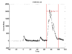
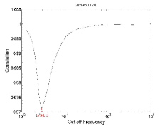
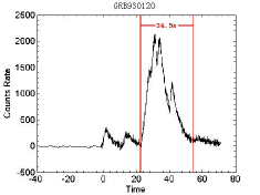
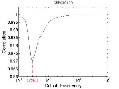
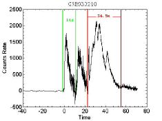
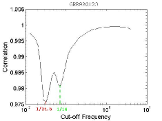
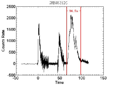
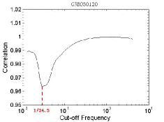
We take GRB 930120 as an example in Group II (gaps/long tails). As shown in Fig.8(a), the burst has two brief activities with durations $\sim 10$ s, followed by the main emission episode. The three episodes are separated by two gaps. The SFC curve (Fig.8(b)) shows only one dip, which corresponds to the main pulse with duration around $34.5$ s.

The puzzling fact is that the $\sim 10$ s feature and the high-frequency spikes overlapping the main pulse are not captured. The missing high-frequency spiky component is due to the low amplitude of this component. The lack of the $\sim 10$ s component may be understood in two ways. (1) The amplitudes of those two pulses are too small compared with the main pulse; (2) The existence of the gaps modified the durations of those pulses from $\sim 10$ s to $\sim 30$ s, which is close to the duration of the main pulse so that the two dips merge to one. To test these possibilities, we perform several tests. First, we manually remove the quiescent periods (the gaps) in the lightcurve. The SFC curve still does not show the $\sim 10$ s component (Fig.8(c,d)). Next, we manually increase the amplitudes of the two pulses to be comparable to that of the main pulse, the $\sim 10$ s component then shows up in the SFC curve (Fig.8(e,f)). Finally, we increase the amplitude of the two pulses but do not remove the gaps. The $\sim 10$ s dip in the SFC curve disappears again (Fig.8(g,h)). This suggests that both reasons (low amplitude and influence of gaps) play a role in missing the $\sim 10$ s component in the original lightcurve.

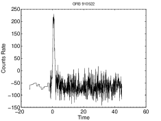
In the irregular group (III) we chose GRB 910522 as an example. The lightcurve is very noisy (Fig.8(i)), and the SFC curve is irregular (Fig.8(j)).

Finally, the group IV includes bursts with short durations or poor temporal resolution. The SFC method is no longer applicable to these bursts. An example (GRB 920718B) is presented in Fig.8(k,l).

Figure 8.— The top and middle panel are original and synthetic lightcurve for GRB930120. The pulses that correspond to the identified frequencies are marked in different colors in the lightcurves. The time scales are rounded to the nearest 0.5. The bottom panel is lightcurve and SFC curve for GRB910522 and GRB920718B.

References

- Barthelmy et al. (2005) Barthelmy, S. D., et al. 2005, ApJ, 635, L133
- Beloborodov et al. (1998) Beloborodov, A. M., Stern, B. E., & Svensson, R. 1998, ApJ, 508, L25
- Beloborodov et al. (2000) Beloborodov, A. M., Stern, B. E., & Svensson, R. 2000, ApJ, 535, 158
- Daigne & Mochkovitch (2003) Daigne, F., & Mochkovitch, R. 2003, MNRAS, 342, 587
- Dermer & Mitman (1999) Dermer, C. D., & Mitman, K. E. 1999, ApJ, 513, L5
- Fishman & Meegan (1995) Fishman, G. J., & Meegan, C. A. 1995, ARA&A, 33, 415
- Golenetskii et al. (2009) Golenetskii, S., Aptekar, R., Mazets, E., Pal’Shin, V., Frederiks, D., Oleynik, P., Ulanov, M., & Svinkin, D. 2009, GRB Coordinates Network, 9647, 1
- Kaneko et al. (2006) Kaneko, Y., Preece, R. D., Briggs, M. S., Paciesas, W. S., Meegan, C. A., & Band, D. L. 2006, ApJS, 166, 298
- Kobayashi et al. (1997) Kobayashi, S., Piran, T., & Sari, R. 1997, ApJ, 490, 92
- Kocevski et al. (2003) Kocevski, D., Ryde, F., & Liang, E. 2003, ApJ, 596, 389
- Kumar & Narayan (2009) Kumar, P., & Narayan, R. 2009, MNRAS, 395, 472
- Lazzati et al. (2009) Lazzati, D., Morsony, B. J., & Begelman, M. C. 2009, ApJ, 700, L47
- Lei et al. (2007) Lei W.H. et al., 2007, A&A, 468, 563
- Li & Fenimore (1996) Li, H., & Fenimore, E. E. 1996, ApJ, 469, L115
- Lu et al. (2008) Lu Y., Huang Y.F., and Zhang S.N., 2008, ApJ, 684, 1330
- Lyutikov & Blandford (2003) Lyutikov, M., & Blandford, R. 2003, arXiv:astro-ph/0312347
- Maxham & Zhang (2009) Maxham, A., & Zhang, B. 2009, ApJ, 707, 1623
- McBreen et al. (2001) McBreen, S., Quilligan, F., McBreen, B., Hanlon, L., & Watson, D. 2001, A&A, 380, L31
- Mészáros & Rees (1993) Mészáros, P., & Rees, M. J. 1993, ApJ, 405, 278
- Morsony et al. (2010) Morsony, B. J., Lazzati, D., & Begelman, M. C. 2010, ApJ, 723, 267
- Nakar& Piran (2002) Nakar, E., & Piran, T. 2002, MNRAS, 331, 40
- Narayan & Kumar (2009) Narayan, R., & Kumar, P. 2009, MNRAS, 394, L117
- Norris et al. (1996) Norris, J. P., Nemiroff, R. J., Bonnell, J. T., Scargle, J. D., Kouveliotou, C., Paciesas, W. S., Meegan, C. A., & Fishman, G. J. 1996, ApJ, 459, 393
- Norris et al. (2000) Norris, J. P., Marani, G. F., & Bonnell, J. T. 2000, ApJ, 534, 248
- Oppenheim et al. (1998) Oppenheim, A.V., Schafer, R.W., Buck, J.R., 1998, ”Discrete-time signal processing” second edit, Vol.2, 52
- Portegies Zwart et al. (1999) Portegies Zwart, S. F., Lee, C.-H., & Lee, H. K. 1999, ApJ, 520, 666
- Piran (1999) Piran, T. 1999, Phys. Rep., 314, 575
- Ramirez-Ruiz et al. (2001) Ramirez-Ruiz, E., Merloni, A., Rees, M. J. 2001, MNRAS, 324, 1147
- Rees & Mészáros (1994) Rees, M. J., & Mészáros, P. 1994, ApJ, 430, L93
- Sari & Piran (1997) Sari, R., & Piran, T. 1997, ApJ, 485, 270
- Shen & Song (2003) Shen, R.-F., & Song, L.-M. 2003, PASJ, 55, 345
- Tagliaferri et al. (2005) Tagliaferri, G., et al. 2005, Nature, 436, 985
- Vetere et al. (2006) Vetere, L., Massaro, E., Costa, E., Soffitta, P., & Ventura, G. 2006, A&A, 447, 499
- Zhang et al. (2006) Zhang, B., Fan, Y. Z., Dyks, J., Kobayashi, S., Mészáros, P., Burrows, D. N., Nousek, J. A., & Gehrels, N. 2006, ApJ, 642, 354
- Zhang & Yan (2011) Zhang, B., & Yan, H. 2011, ApJ, 726, 90
- Zhang & Zhang (2011) Zhang, B., & Zhang, B. 2011, MNRAS, to be submitted
- Zhang et al. (2003) Zhang, W., Woosley, S. E., & MacFadyen, A. I. 2003, ApJ, 586, 356