Bulk-boundary correspondence in three dimensional topological insulators

Abstract

We discuss the relation between bulk topological invariants and the spectrum of surface states in three dimensional non-interacting topological insulators. By studying particular models, and considering general boundary conditions for the electron wavefunction on the crystal surface, we demonstrate that using experimental techniques that probe surface states, only strong topological and trivial insulating phases can be distinguished; the latter state being equivalent to a weak topological insulator. In a strong topological insulator, only the parity of the number of surface states, but not the number itself, is robust against time-reversal invariant boundary perturbations. Our results suggest a $\mathbb{Z}_{2}$ definition of the bulk-boundary correspondence, compatible with the $\mathbb{Z}_{2}$ classification of topological insulators.

I Introduction

The defining characteristic of an electric insulator is the existence of an energy gap to charge excitations. Depending on the physical origin of that gap insulating materials are broadly divided into two classes: Mott insulators with the gap having an origin in the electron interactions, and band insulators, where the gap originates essentially from the single particle energy terms, with many-body effects simply renormalizing the bare band parameters. Because of their single-particle nature band insulators are often thought to be the simplest systems, whose electronic properties are adequately described by the usual quantum theory of solids Landau_IX . Recently, however, a classification of these materials has emerged Kane_colloquium ; Moore_3DTI , based on topological invariants Thouless_1998 , which characterize their band structure. In particular, it was shown Kane_Z2 ; Zhang_MEE that spin-orbit (SO) interaction and time-reversal symmetry can stabilize topologically non-trivial electronic states in certain systems, which were thus termed topological insulators (TI). An experimental signature of these phases is the presence of chiral metallic surface states, which are claimed to be robust against time-reversal invariant local perturbations and weak disorder. Surface states were indeed observed in bismuth antimony alloys Moore_3DTI , as well as in the ${\rm Bi_{2}X_{3}}$ and ${\rm Sb_{2}X_{3}}$, with ${\rm X=(Se,Te)}$, families Zhang_2009 ; Hsieh_2009 .

The bulk-boundary correspondence is a physical concept which relates topological properties of the bulk with the number of gapless edge modes. This relation has generated a lot of discussion in the context of Quantum Hall Effect Halperin_1982 ; Hatsugai_1993 , graphene Hatsugai_2007 , and now TI Kane_Z2 ; Zhang_MEE ; Zhang_2006 ; Mong_2011 . In particular, in Ref. Kane_Z2, it was argued that a two-dimensional TI is characterized by an odd number of metallic edge states. Qualitatively, due to time-reversal symmetry, surface states in STI do not back-scatter and thus, can not be easily localized, becoming robust against local time-reversal invariant perturbations. In three dimensions (3D) it is argued that one should distinguish Kane_Z2 among strong and weak TI (STI and WTI) states, where the Fermi arc encloses an odd or even number of surface Dirac (i.e. Kramers-degenerate) points, respectively.

So far the bulk-boundary correspondence remains a quite loosely formulated conjecture. It remains unclear how universally valid is this conjecture in real many-body insulating systems, or how robust is this correspondence with respect to variations in the surface properties of those systems. In any bulk-boundary correspondence specific properties of the surface should be of relevance. Indeed, the electronic edge spectrum can be very sensitive Volkov_1981 to the specific form of the effective surface Hamiltonian. For example, in the context of graphene the connection between the valley-specific Hall conductivity and the number of gapless edge modes has been found to be dependent upon the boundary conditions (BC) Martin_2010 .

In the present paper we examine the bulk-boundary correspondence in 3D band insulators with strong SO interaction. We present a technique to analyze their surface spectra based on the ideas of Ref. Satanin_1984, , developed in the context of semiconductor nanostructures, and study the effect of variations in BC on the spectrum of surface states. In particular, we use algebraic properties of the model Hamiltonian to construct BC according to symmetries of the problem, such as time-reversal invariance. We also discuss the role of symmetry-breaking surface perturbations. Our work leads to a two-fold result. On the one hand, we show that even in a clean system with no surface reconstruction, from the standpoint of the surface spectra, there exists no physical distinction between WTI and topologically trivial insulating phases. In particular, we present examples of trivial insulators, which would appear as WTIs, since they also possess an even number of surface Dirac cones. On the other hand, the STI state is robust against time-reversal invariant boundary perturbations, in the sense that the Fermi arc always encloses an odd number of surface Dirac points with an odd number of edge states crossing the Fermi level along a path between two time-reversal invariant momenta (TRIMs) in the surface Brillouin zone. The number of crossings depends on the particular choice of BC. This indicates that edge states in a STI are not robust against arbitrary time-reversal invariant surface perturbations. However, the parity of their number is protected.

These observations provide a $\mathbb{Z}_{2}$ formulation of the bulk-boundary correspondence in 3D TI:

$$\nu_{0}=N_{s}\,\,{\rm mod}\,\,2,$$

where $\nu_{0}$ is the strong $\mathbb{Z}_{2}$ bulk topological invariant Kane_Z2 , $N_{s}$ is the number of Kramers-degenerate points in the surface Brillouin zone enclosed by the Fermi arc, and we assume that there are no time-reversal breaking perturbations at the insulator’s surface. This relation shows that it is only appropriate to differentiate between STI and trivial insulating phases, characterized by $\nu_{0}=1$ and $\nu_{0}=0$, respectively. From an experimental point of view (by looking at the spectrum of surface states), a WTI is equivalent to a trivial insulator as will be shown.

The paper is organized as follows. In the next section we consider a simple example of a trivial insulator and show that under certain conditions it may possess an even number of metallic edge states, thus appearing as a WTI. In Sec. III we discuss the robustness of surface states in a model of a STI, and demonstrate the protection of parity of their number, but not the number or the states themselves. Moreover, we further discuss the indistinguishability between a WTI and a trivial insulator from the standpoint of the number of edge (surface) modes. In Sec. IV, we study the effect of time-reversal breaking surface perturbations on the edge spectrum of a STI. Our conclusions are summarized in Sec. V.

II Dirac-like band model

The SO interaction plays an important role in establishing a band structure characterized by non-trivial topological invariants. Physically, this means that proper interband matrix elements of the SO term in the Hamiltonian must be comparable with the bulk band gap, so that the bands become essentially non-parabolic. As a ubiquitous consequence of the band mixing, Dirac-like bulk spectra of electrons and holes are formed Bir_Pikus . In this section we consider a simple model of a topologically trivial insulator, which neverthless would look like a WTI in the sense that the Fermi arc encloses an even number of surface Dirac points. We also show that the existence of edge states is very sensitive to the BC, imposed on the single-particle wavefunction at the crystal surface.

II.1 General formalism

The simplest lattice model, which contains SO interaction naturally, is just the tight-binding form of the Dirac Hamiltonian:

$$H_{D}=\frac{\lambda}{2{\rm i}}\sum_{i,\mu}\bigl{(}\Psi^{\dagger}_{i}\alpha^{\mu}\Psi_{i+\mu}{\rm e}^{{\rm i}\theta^{\mu}_{i}}-{\rm h.c.}\bigr{)}+\epsilon\sum_{i}\Psi^{\dagger}_{i}\beta\Psi_{i},$$ (1)

where from now on subindex $i\equiv{\bm{x}}_{i}=(x_{i},y_{i},z_{i})$ enumerates sites of a simple cubic lattice; $i+\mu\equiv\mu_{i}+1$ with $\mu=x,y,z$; $\Psi_{i}=(c_{ic\sigma},c_{iv\sigma})$ destroys an electron with spin $\sigma$ in the conduction ($c$) or valence ($v$) band; $\lambda$ and $\epsilon$ are the SO coupling constant and band gap, respectively; and $\theta^{\mu}_{i}$ is a $U(1)$ gauge field. The Dirac matrices $\beta$ and $\alpha^{\mu}$ have the well-known properties Akhiezer_Berestetskii :

$$\{\alpha^{\mu},\alpha^{\nu}\}=2\delta_{\mu\nu}; \,\,\{\alpha^{\mu},\beta\}=0;\,\,[\alpha^{\mu},\alpha^{\nu}]=2{\rm i}\varepsilon_{\mu\nu\kappa}\Sigma_{\kappa};$$

$$(\alpha^{\mu})^{2}=\beta^{2}=1$$

with $\Sigma_{\mu}=(1\otimes\sigma^{\mu})$ being the 4-spin operator, $\sigma^{\mu}$ – the Pauli matrix, and $\varepsilon_{\mu\nu\kappa}$ – the Lévi-Civita symbol. From Eq. (1) it is easy to obtain an expression for the charge current, as a variation of the Hamiltonian with respect to the gauge field:

$$J^{\mu}_{i}\equiv\frac{\delta H_{D}}{\lambda\delta\theta^{\mu}_{i}}\bigg{|}_{\theta^{\mu}_{i}=0}=\frac{1}{2}\bigl{(}\Psi^{\dagger}_{i}\alpha^{\mu}\Psi_{i+\mu}+\Psi^{\dagger}_{i+\mu}\alpha^{\mu}\Psi_{i}\bigr{)}.$$ (2)

In the rest of this section, we assume that $\theta_{i}^{\mu}=0$.

The Hamiltonian of Eq. (1) commutes with the time-reversal (${\cal T}$) and space inversion (${\cal P}$) operators. Also, the bulk band structure is invariant under interchange of the conduction and valence bands, which means that $H_{D}$ has the charge-conjugation (${\cal C}$) symmetry. These three operations are defined by their action on a single-particle orbital $\psi(t,{\bm{x}}_{i})=\psi_{i}(t)$ Akhiezer_Berestetskii :

$${\cal T}\psi(t,{\bm{x}}_{i})=\alpha^{x} \alpha^{z}\psi^{*}(-t,{\bm{x}}_{i});\,\,{\cal P}\psi(t,{\bm{x}}_{i})=\beta\psi(t,-{\bm{x}}_{i});$$

$${\cal C}\psi(t,{\bm{x}}_{i})=\beta\alpha^{y}\psi^{*}(t,{\bm{x}}_{i}).$$

Motion in an infinite crystal also preserves the tensor spin operator Satanin_1984 ; Bagrov_Gitman :

$$T_{\mu}=\frac{\varepsilon_{\mu\nu\kappa}}{2{\rm i}}\sum_{i}\bigl{(}\Psi^{\dagger}_{i}\beta\Sigma_{\nu}\Psi_{i+\kappa}-{\rm h.c.}\bigr{)}.$$ (3)

It follows that ${\bm{T}}$ is a polar, time-reversal invariant vector.

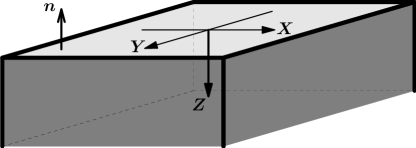
Figure 1: Geometry of the problem studied in this paper. The crystal is bounded by the plane $z_{i}=0$ and occupies the half-space $z_{i}>0$. The unit vector ${\bm{n}}$ denotes an outer normal to the surface.

In order to study the spectrum of surface states, we now consider a half-infinite crystal, bounded by the plane $z_{i}=0$ and occupying the region $z_{i}>0$ (see Fig. 1). On the surface the single-particle wavefunction $\psi_{i}$ will satisfy a linear relation of the form:

$$-\sum_{\mu}n_{\mu}\psi_{i_{s}+\mu}+S\psi_{i_{s}}=0,$$ (4)

where ${\bm{n}}$ is the outer normal to the surface and $i_{s}$ denotes lattice sites on the surface. The general structure of the $4\times 4$ boundary matrix $S$ is fixed by requirements Volkov_1981 ; Satanin_1984 that the current $\langle{\bm{J}}_{0}\cdot{\bm{n}}\rangle$ through the surface vanishes, and the fundamental symmetries ${\cal T}$ and ${\cal P}$ are preserved:

$$S=\xi_{0}\beta+{\rm i}\xi_{1}\beta{\bm{\alpha}}\cdot{\bm{n}}.$$ (5)

In this expression the parameters $\xi_{0,1}$ are free. At the phenomenological level, they encode various surface properties. For example, the first term in Eq. (5) changes sign under charge conjugation ${\cal C}$, which physically means that at the boundary there is a mixing (whose amount is controlled by $\xi_{0}$) of the bulk Bloch bands. Similarly, the second term in $S$ describes the intensity of SO interaction at the surface, which is caused by rapid changes in the crystal field. Thus, after scattering from the surface an electron acquires an extra phase, due to spin rotation. Since the localized (Tamm) states at the crystal boundary are formed as a result of interference of bulk Bloch states Tamm_1932 , this term has a profound effect on their stability. We also note that the BC (5) is translationally invariant along the surface.

In the bounded crystal in Fig. 1, only the normal to the surface component of ${\bm{T}}$ [Eq. (3)] is conserved. In ${\bm{k}}$-space (${\bm{k}}$ is the crystal momentum) it can be written as:

$$T_{z}=\sum_{{\bm{k}}_{\perp},z_{i}}\Psi^{\dagger}_{z_{i}}({\bm{k}}_{\perp})t^{z}({\bm{k}}_{\perp})\Psi_{z_{i}}({\bm{k}}_{\perp})$$

with ${\bm{k}}_{\perp}=(k_{x},k_{y})$, and

$$t^{z}({\bm{k}}_{\perp})=\beta\bigl{(}\Sigma_{x}\sin k_{y}-\Sigma_{y}\sin k_{x}\bigr{)}.$$

The eigenstates of $t^{z}({\bm{k}}_{\perp})$ have the form:

$$\psi_{\tau{\bm{k}}_{\perp}}(z_{i})=\begin{pmatrix}\varphi_{\tau{\bm{k}}_{\perp}}(z_{i})U_{\tau{\bm{k}}_{\perp}}\\ \chi_{\tau{\bm{k}}_{\perp}}(z_{i})U_{-\tau{\bm{k}}_{\perp}}\end{pmatrix},$$ (6)

where

$$U_{\tau{\bm{k}}_{\perp}}=\frac{1}{\sqrt{2}}\begin{pmatrix}1\\ -\frac{{\rm i}\tau}{s_{\perp}}(\sin k_{x}+{\rm i}\sin k_{y})\end{pmatrix},$$

$\tau=\pm 1$, $s_{\perp}=\sqrt{\sin^{2}k_{x}+\sin^{2}k_{y}}$, and the amplitudes $\varphi$ and $\chi$ are arbitrary. The corresponding eigenvalues are $\tau s_{\perp}$. The $z$-independent part of the kinetic energy in Eq. (1) can be expressed in terms of $t^{z}({\bm{k}}_{\perp})$:

$$\frac{\lambda}{2{\rm i}}\sum_{i,\mu=(x,y)}\bigl{(}\Psi^{\dagger}_{i}\alpha^{\mu} \Psi_{i+\mu}-{\rm h.c.}\bigr{)}=$$

$$={\rm i}\lambda\sum_{{\bm{k}}_{\perp},z_{i}}\Psi^{\dagger}_{{\bm{k}}_{\perp}z_{i}}\beta\alpha^{z}t^{z}({\bm{k}}_{\perp})\Psi_{{\bm{k}}_{\perp}z_{i}}.$$

This fact has two important consequences: (i) The problem becomes effectively one-dimensional and we can work with two-component wavefunctions, similar to the case of a spherically symmetric field Akhiezer_Berestetskii :

$$\begin{pmatrix}\varphi_{\tau{\bm{k}}_{\perp}}(z_{i})U_{\tau{\bm{k}}_{\perp}}\\ \chi_{\tau{\bm{k}}_{\perp}}(z_{i})U_{-\tau{\bm{k}}_{\perp}}\end{pmatrix}\to\begin{pmatrix}\varphi_{\tau{\bm{k}}_{\perp}}(z_{i})\\ \chi_{\tau{\bm{k}}_{\perp}}(z_{i})\end{pmatrix}.$$

(ii) We are free to choose a representation for the Dirac matrices $\beta$ and $\alpha^{z}$. In the rest of the section, we use the following identification:

$$\beta\to\sigma^{z};\quad\alpha^{z}\to\sigma^{x}.$$

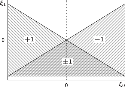
Figure 2: Stability regions of edge states, obtained from Eq. (7). Inside shaded areas there exist surface states with at least one value of the polarization $\tau$, as indicated by the numbers $\pm 1$. The boundaries of shaded regions are given by the expression $\xi_{1}=-(\lambda\tau s_{\perp}/\epsilon)\xi_{0}$.

II.2 Surface spectrum

In order to obtain the edge (surface) spectrum, we follow the method of Ref. Tamm_1932, . First, let us consider the bulk band structure:

$$\varepsilon_{{\bm{k}}_{\perp},k_{z}}=\pm\sqrt{\epsilon^{2}+\lambda^{2}(s_{\perp}^{2}+\sin^{2}k_{z})}.$$

A surface state will have a complex-valued $k_{z}=p+{\rm i}q$ with $p$ and $q$ chosen in such a way that ${\rm Im}\,\varepsilon=0$. Since $q\neq 0$, one obtains: (i) $p=0$ or $p=\pi$, and (ii) $p=\pm\pi/2$. Only in case (i) the state has an energy inside the band gap. Therefore, a general (two-component) wavefunction, decaying into the crystal ($z_{i}>0$), can now be written as a linear combination:

$$\psi_{\tau{\bm{k}}_{\perp}}(z_{i})=\sum_{p=0,\pi}c_{p}\begin{pmatrix}\varepsilon+\epsilon\\ {\rm i}\lambda({\rm e}^{{\rm i}p}{\rm sh}\,q-\tau s_{\perp})\end{pmatrix}\biggr{)}{\rm e}^{({\rm i}p-q)z_{i}}.$$

Imposing the BC of Eqs. (4) and (5) one easily obtains the inverse localization length $q$ of the state (cf. Ref. Volkov_1981, ):

$${\rm sh}^{2}q_{\tau{\bm{k}}_{\perp}}=\frac{r\varrho_{\tau}-1/2+\sqrt{(\varrho_{\tau}-r/2)^{2}+(1-r^{2})/4}}{1-r^{2}},$$ (7)

which defines the surface state dispersion relation via $\varepsilon_{\tau{\bm{k}}_{\perp}}=\pm\sqrt{\epsilon^{2}+\lambda^{2}(s_{\perp}^{2}-{\rm sh}^{2}q_{\tau{\bm{k}}_{\perp}})}$. In this expression:

$$\varrho_{\tau}(\xi_{0},\xi_{1})= (1-r)(\tau s_{\perp}\xi_{0}+\epsilon\xi_{1}/\lambda);$$

$$r(\xi_{0},\xi_{1})= \frac{\xi_{0}^{2}+\xi_{1}^{2}-1}{\xi_{0}^{2}+\xi_{1}^{2}+1}\in(-1,1).$$

A surface state exists only if $q>0$, which is equivalent to $\varrho_{\tau}<0$. Regions in the plane $(\xi_{0},\xi_{1})$, where this inequality is satisfied, are shown in Fig. 2. For a given point inside a shaded area, there is a solution either with one, or both values of $\tau$. Moreover, there is an unshaded region, where the edge spectrum disappears. In general, the surface states are gapped. However, this gap closes at some points in Fig. 2. For example, let us consider the case $\xi_{0}=0$, $\xi_{1}<0$ and $r=-\eta/\sqrt{1+\eta^{2}}$ with $\eta=\epsilon/\lambda>0$. Then, solutions for $p=0$ and $\pi$ disentagle. Therefore, ${\rm sh}\,q_{\tau{\bm{k}}_{\perp}}=\eta$, $\varepsilon^{p}_{\tau{\bm{k}}_{\perp}}=\lambda{\rm e}^{{\rm i}p}\tau s_{\perp}=\pm\lambda\tau s_{\perp}$, and the wavefunction is:

$$\psi_{\tau{\bm{k}}_{\perp}}^{p}(z_{i})=\sqrt{\eta}\begin{pmatrix}1\\ {\rm i}{\rm e}^{{\rm i}p}\end{pmatrix}\bigl{[}-\eta+\sqrt{1+\eta^{2}}\bigr{]}^{z_{i}+\frac{1}{2}}{\rm e}^{{\rm i}pz_{i}}.$$

Since $\varepsilon_{\tau{\bm{k}}_{\perp}}$ depends on ${\bm{k}}_{\perp}$ only through $s_{\perp}$, for the chemical potential inside the band gap, the Fermi arc always encloses an even number of Dirac points. Thus, from an experimental perspective this model system would look like a WTI Kane_Z2 . Nevertheless, it is straightforward to check that all four topological invariants $(\nu_{0}(\nu_{1}\nu_{2}\nu_{3}))$ vanish (we remind the reader that $\nu_{0}=0$ and $(\nu_{1}\nu_{2}\nu_{3})\neq 0$ is the mathematical characterization of a WTI). As we shall see in the next section, the above result is not specific to the model of Eq. (1).

III Lattice Dimmock model

The Dirac model (1) describes a trivial insulator. However, it can be extended to support a STI phase. We consider one such modification, proposed in Ref. Rosenberg_2010, :

$$H=H_{D}-t\sum_{i,\mu}\bigl{(}\Psi^{\dagger}_{i}\beta\Psi_{i+\mu}{\rm e}^{{\rm i}\theta^{\mu}_{i}}+{\rm h.c.}\bigr{)},$$ (8)

where $t>0$ is the hopping amplitude between nearest neighbor sites in a 3D cubic lattice. The model thus defined is a lattice analog of the well-known Dimmock model Dimmock_1964 , which provides an effective-mass description of electronic spectra in lead chalcogenides. The Dirac model, studied in the previous section, is recovered in the limit $t\to 0$. However, the point $t=0$ is singular and the limit has to be taken carefully.

Depending on the ratio of $\epsilon/t$, the model (8) exhibits the following phases Rosenberg_2010 : (i) STI if $2t<|\epsilon|<6t$, (ii) WTI for $|\epsilon|<2t$ and (iii) the trivial band insulator when $|\epsilon|>6t$. In the STI phase the Fermi energy inside the gap must cross an odd number of edge states along a path between two time-reversal invariant momenta in the surface Brillouin zone. Indeed, it was shown a long time ago that in the long wavelength approximation under band inversion the Dimmock model has exactly one Dirac cone at the surface Kisin_1987 . This conclusion is in agreement with the phase diagram, because in the continuum limit the band gap $\Delta=\epsilon-6t$ is negative for $\epsilon\lesssim 6t$. In this section we study the effect of variations in the BC on the surface spectrum of the lattice Dimmock model, and on the physical meaning of the above phase diagram.

As before, we start by deriving the BC with given symmetry properties. The probability current

$$J^{\mu}_{i}= \frac{1}{2}\bigl{(}\Psi^{\dagger}_{i}\alpha^{\mu}\Psi_{i+\mu}+\Psi^{\dagger}_{i+\mu}\alpha^{\mu}\Psi_{i}\bigr{)}$$

$$-\frac{{\rm i}t}{\lambda}\bigl{(}\Psi^{\dagger}_{i}\beta\Psi_{i+\mu}-\Psi^{\dagger}_{i+\mu}\beta\Psi_{i}\bigr{)}.$$ (9)

vanishes at the surface if the wavefunction satisfies the constraint (4) with a boundary operator of the form:

$$S=\frac{2t}{\lambda}\xi_{0}+\xi_{1}\beta+{\rm i}\xi_{0}\beta{\bm{\alpha}}\cdot{\bm{n}}.$$ (10)

The discussion presented after Eq. (5) regarding the physical meaning of individual terms is fully applicable here as well.

It is easy to see that the lattice Dimmock model (8) has the same symmetries as the Dirac model of the previous section. Therefore, the problem of determining the surface spectrum, in the geometry of Fig. 1, again becomes one-dimensional. However, now it is convenient to choose a different representation of the Dirac matrices:

$$\alpha^{z}\to\sigma^{y};\quad\beta\to\sigma^{x}.$$ (11)

We also introduce a notation $\epsilon_{\perp}=\epsilon-2t(\cos k_{x}+\cos k_{y})$.

The bulk band structure has the form:

$$\varepsilon_{{\bm{k}}_{\perp},k_{z}}=\pm\sqrt{(\epsilon_{\perp}-2t\cos k_{z})^{2}+\lambda^{2}(s_{\perp}^{2}+\sin^{2}k_{z})}.$$

The requirement ${\rm Im}\,\varepsilon=0$ is equivalent to the equation ${\rm Im}\,\varepsilon^{2}=0$ under the condition ${\rm Re}\,\varepsilon^{2}\geqslant 0$. In the complex $k_{z}$-plane ($k_{z}=p+{\rm i}q$) ${\rm Im}\,\varepsilon^{2}$ vanishes when: (i) $p=0$, (ii) $p=\pi$ and (iii) along the line $\cos p\,{\rm ch}\,q=2t\epsilon_{\perp}/\bigl{[}(2t)^{2}-\lambda^{2}\bigr{]}$. In general, a surface state wavefunction is a complicated function with a ${\bm{k}}_{\perp}$-dependent complex localization length. However, there exists a parameter range, where the edge states are purely evanescent, i.e. $p=0$. Indeed, let us assume that

$$4t<\epsilon<10t;\quad(2t)^{2}-\frac{1}{3}(\epsilon-4t)^{2}\leqslant\lambda^{2}\leqslant(2t)^{2}.$$ (12)

Then, possible values of $q$ are given by:

$${\rm ch}\,q_{1,2}= \frac{2t\epsilon_{\perp}}{(2t)^{2}-\lambda^{2}}$$

$$\mp\frac{\sqrt{\epsilon_{\perp}^{2}\lambda^{2}+\bigl{[}\varepsilon^{2}-\lambda^{2}(s_{\perp}^{2}+1)\bigr{]}\bigl{[}(2t)^{2}-\lambda^{2}\bigr{]}}}{(2t)^{2}-\lambda^{2}}.$$

We note that because of peculiar properties of the band structure, in the present model there always exists a partial evanescent solution with ${\rm ch}\,q_{2}>1$. However, by virtue of Eq. (12) both ${\rm ch}\,q_{1,2}\geqslant 1$, with $q_{1}$ being the inverse localization length of a state. Using the form (11) of $\alpha^{z}$ and $\beta$, the general localized solution can be written as:

$$\psi_{\tau{\bm{k}}_{\perp}}(z_{i})=\sum_{a=1,2}c_{a}\begin{pmatrix}\epsilon_{\perp}-2t{\rm ch}\,q_{a}+\lambda{\rm sh}\,q_{a}\\ \varepsilon+\lambda\tau s_{\perp}\end{pmatrix}{\rm e}^{-q_{a}z_{i}}.$$

Before considering generic BC (10), let us analyze the case $\xi_{1}=0$, when there is no band mixing at the boundary. One can easily show that there exists a surface state with energy $\varepsilon_{\tau{\bm{k}}_{\perp}}=\lambda\tau s_{\perp}$, and momentum $q$

$${\rm ch}\,q_{1,2}=\frac{2t\epsilon_{\perp}}{(2t)^{2}-\lambda^{2}}\mp\frac{\sqrt{\lambda^{2}\epsilon_{\perp}^{2}-\lambda^{2}\bigl{[}(2t)^{2}-\lambda^{2}\bigr{]}}}{(2t)^{2}-\lambda^{2}},$$ (13)

with the resulting wavefunction

$$\psi_{\tau{\bm{k}}_{\perp}}(z_{i})\sim\begin{pmatrix}0\\ 1\end{pmatrix}\bigl{(}{\rm e}^{-q_{1}z_{i}}-\eta(\xi_{0}){\rm e}^{-q_{2}z_{i}}\bigr{)},$$ (14)

where $\eta(\xi_{0})=\bigl{[}\bigl{(}2t/\lambda-1\bigr{)}\xi_{0}+{\rm e}^{-q_{1}}\bigr{]}/\bigl{[}\bigl{(}2t/\lambda-1\bigr{)}\xi_{0}+{\rm e}^{-q_{2}}\bigr{]}$. This state exists only in a region of ${\bm{k}}_{\perp}$-space, defined by $\epsilon_{\perp}\leqslant 2t$. At the boundary of this region $q_{1}=0$, and the state merges into the bulk continuum. Clearly, the above condition is a priori false when $\epsilon>6t$, in agreement with the general phase diagram Rosenberg_2010 .

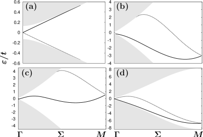
Figure 3: Surface spectra of the lattice Dimmock model for different values of the parameters $\xi_{0,1}$ and $\epsilon/t$. SO interaction is $\lambda/t=\sqrt{3}$. The spectra are plotted along the path $(0,0)$-$(k_{x},k_{y})$-$(\pi,\pi)$ in the surface Brillouin zone. The shaded regions describe the bulk continuum with the band gap equal to $|\epsilon-6t|$. In panel (a) the plot is actually truncated before the $M$-point is reached, for readability. Solid lines represent $\tau=+1$, dashed lines $\tau=-1$. (a) $\xi_{0}=1.0$, $\xi_{1}=0.0$; (b) $\xi_{0}=0.0$, $\xi_{1}=0.1$; (c) $\xi_{0}=0.0$, $\xi_{1}=0.045$; (d) $\xi_{0}=0.1$, $\xi_{1}=0.3$. Panels (a)–(c) correspond to a STI with $\epsilon/t=5.87$, panel (d) describes a trivial insulator with $\epsilon/t=6.37$.

When $\xi_{0,1}\neq 0$ we observe that matrices $1$, $\beta$ and ${\rm i}\beta{\bm{\alpha}}\cdot{\bm{n}}$ consitute an orthonormal (though not closed) set $\{m_{i}\}$: ${\rm Tr}\,m_{i}m_{j}=4\delta_{ij}$, $m_{i}^{2}=1$. Thus, for any value of $\xi_{1}$ there exists a unitary transformation ${\cal U}(\omega)=\exp{\bigl{(}{\rm i}\omega{\bm{\alpha}}\cdot{\bm{n}}/2\bigr{)}}$, which diagonalizes $S$ (cf. the discussion of the case $\xi_{1}=0$). For example, in the representation (11):

$${\cal U}^{\dagger}S(\xi_{0},\xi_{1})\,{\cal U}=\frac{2t}{\lambda}\xi_{0}+{\rm i}\sqrt{\xi_{0}^{2}+\xi_{1}^{2}}\,\beta{\bm{\alpha}}\cdot{\bm{n}}\equiv S_{\cal U}.$$

The problem of determining the edge spectrum of the original Hamiltonian $H$ [Eq. (8)] with the BC $S_{\cal U}$ is mathematically identical to the analysis, which led to Eq. (13). Of course, the transformation ${\cal U}$ changes $H$ as well: $H\to H_{\cal U}\neq H$, but leaves its topological structure intact. Qualitatively, variations in the boundary parameters $\xi_{0,1}$ can be seen as unitary transformations of the bulk Hamiltonian. These transformations also guarantee that the BC is kept diagonal. If initially the bulk band structure was characterized by a strong topological index $\nu_{0}\neq 0$, the same will be true for $H_{\cal U}$. The shape of the edge spectrum does depend on a particular choice of $\xi_{0,1}$ and has to be computed explicitly. However, the above argument implies that if at $\xi_{1}=0$, the Fermi arc enclosed an odd number (e.g. one) of Kramers-degenerate points, then the same will be true for any $\xi_{1}$.

In Fig. 3, we present the dispersion relation of surface states for several values of the BC parameters in the STI regime ($\epsilon=5.87t$) and for the trivial insulator ($\epsilon=6.37t$). From panels (a)–(c) it follows that in the STI phase the number of edge states at the Fermi level may change, depending on the BC parameters, but it always remains odd, i.e. the parity of their number is protected. These surface states exist for all values of $\xi_{0,1}$.

Panel (d) corresponds to the case $\epsilon>6t$ when the system is a trivial insulator, which can nevertheless exhibit metallic edge states. The surface spectrum is quite sensitive to the BC parameters and disappears for $\xi_{0,1}\sim 1$. Similar to the problem studied in the previous section, the number of Fermi level crossings is even. This circumstance once again shows the physical indistinguishability of a WTI and a trivial insulator.

IV Effect of time-reversal breaking surface perturbations

Time-reversal symmetry plays a crucial role in stabilizing the STI phase and metallic properties of the surface. When this symmetry is broken via some physical mechanism, the Kramers theorem no longer holds and surface Dirac fermions are expected to acquire mass Kane_Z2 ; Zhang_MEE , i.e. they become gapped. In Ref. Chen_2010, such gapped edge states were indeed observed in ${\rm Bi_{2}Se_{3}}$ when doped with magnetic impurities at the surface.

Phenomenologically, we can simulate this effect by adding a ${\cal T}$-breaking perturbation to the boundary operator $S$. Let us consider one such term:

$$\Delta S=\xi_{\cal T}\beta\gamma_{5}{\bm{\alpha}}\cdot{\bm{n}},$$ (15)

where $\gamma_{5}={\rm i}\alpha^{x}\alpha^{y}\alpha^{z}$ is the pseudo-scalar matrix Akhiezer_Berestetskii . Because of this matrix, the correction (15) also breaks space inversion symmetry. Nevertheless, it is easy to see that the current (9) vanishes at the surface after $\Delta S$ has been added to the boundary operator (10).

Since the operator $T_{z}$, introduced in Sec. II, is invariant under time-reversal, $\Delta S$ will mix states with different values of $\tau$. In the absence of a natural conserved quantity, suitable for labelling single-electron states, the complete investigation of the edge spectrum becomes quite cumbersome. Still, one can understand the qualitative effect of $\Delta S$ by working in the perturbative regime, i.e. when $|\xi_{\cal T}|$ is small. In order to simplify things even further, we confine our analysis to a particular case, when there is no band mixing at the surface, i.e. $\xi_{1}=0$ in (10). Then, we can use ideas of the previous section to transfer the ${\cal T}$-breaking term from the BC to the bulk Hamiltonian via a unitary transformation ${\cal U}_{\cal T}$, and employ degenerate perturbation theory to treat the resulting corrections in the Hamiltonian within the subspace of edge states (14).

The unitary transformation ${\cal U}_{\cal T}$ is effected by $\gamma_{5}$ [cf. Eq. (10)]:

$${\cal U}_{\cal T}={\rm e}^{{\rm i}\omega\gamma_{5}/2};\quad{\rm tg}\,\omega=\xi_{\cal T}/\xi_{0}.$$

To first order in $\xi_{\cal T}$, the boundary operator (10) remains unchanged, and the only correction to the Hamiltonian (8) is:

$$\Delta H=\frac{\xi_{\cal T}}{\xi_{0}}\biggl{[}\epsilon\sum_{i}\Psi^{\dagger}_{i}\Gamma\Psi_{i}-t\sum_{i,\mu}\bigl{(}\Psi^{\dagger}_{i}\Gamma\Psi_{i+\mu}+{\rm h.c.}\bigr{)}\biggr{]}$$

with $\Gamma={\rm i}\beta\gamma_{5}$. In the basis (14) the matrix elements of $\Delta H$ can be written as:

$$\langle\psi_{\tau^{\prime}{\bm{k}}_{\perp}}|\Delta H|\psi_{\tau{\bm{k}}_{\perp}}\rangle\sim\epsilon\bigl{(}\xi_{\cal T}/\xi_{0}\bigr{)}\sigma^{x}_{\tau^{\prime}\tau}.$$

Therefore, at ${\bm{k}}_{\perp}=0$ (Dirac point) the perturbation (15) opens a gap $\Delta_{\cal T}\sim|\xi_{\cal T}/\xi_{0}|$, in qualitative agreement with the experiments of Ref. Chen_2010, .

V Conclusion

Since in real materials the electronic structure of the surface is largerly unknown, investigation of the surface properties, such as the spectrum of localized states, requires a phenomenological approach similar to the one employed in the present work. It is important to realize that any bulk-boundary correspondence cannot be simply based on general topological arguments that disregard hypotheses about the boundary conditions used. The key idea of our method consists of using the algebraic structure of the bulk Hamiltonian to classify boundary conditions for the Bloch wavefunctions according to fundamental symmetries of the problem.

When the surface preserves time-reversal symmetry, our results suggest that experimentally, i.e. by looking at the edge spectrum, one can only discriminate between the STI and trivial insulating phases. The claimed experimental signature of a WTI – an even number of surface states crossing the Fermi level along a path between two TRIMs Kane_Z2 – turns out to be misleading. Indeed, by adjusting phenomenological parameters in the boundary conditions, one can make a trivial insulator exhibit a surface spectrum similar to that of a WTI, even in a clean system, where the periodicity of the surface is preserved. Therefore, these two phases cannot be physically distinguished by looking at the edge spectrum, and should be theoretically classified as the same state.

On the contrary, in the STI phase the Fermi level crosses an odd number of surface states. This precise number depends on a particular choice of the boundary condition parameters, e.g. it changes from 1 to 3 in panels (a) and (c) of Fig. 3, but its parity is always preserved. Hence, the surface spectrum of a STI (and for the sake of the argument of any band insulator) is not robust against time-reversal invariant boundary perturbations.

These observations can be naturally summarized in a consistent definition of a bulk-boundary correspondence:

$$\nu_{0}=N_{s}\,\,{\rm mod}\,\,2,$$

where $\nu_{0}$ is the strong $\mathbb{Z}_{2}$ bulk topological invariant, introduced by Kane et al. Kane_Z2 and $N_{s}$ is the number of surface Kramers doublets inside the Fermi arc (or the number of edge states crossing the Fermi level along any path between two TRIMs in the surface Brillouin zone). Only the parity of the number of surface states is protected. This definition is compatible with the classification of TIs according to quantization of the axion $\theta$-term Zhang_MEE ; Wang_2010 , which also describes the orbital magneto-electric coupling Essin_2009 .

The bulk topological invariants are meaningful only if the surface preserves time-reversal symmetry. In Sec. IV we demonstrated that a ${\cal T}$-breaking perturbation opens a gap in the edge spectrum at the TRIMs, and effectively destroys the STI phase. This conclusion is in agreement with recent experiments Chen_2010 performed in bismuth selenide with the time-reversal symmetry explicitly broken by surface magnetic impurities.

Finally, we would like to emphasize that our demonstrations are applicable to uncorrelated, i.e. mean-field-like, “TI” systems. The effect of correlations beyond mean-field is still an open problem. While there are some efforts Varney_2010 to extend the existing classification of TIs to interacting systems, so far they only amount to mean-field arguments.

References

- (1) L. P. Pitaevskii and E. M. Lifshitz, Statistical Physics, Part 2, 1st ed., Butterworth-Heinemann, Oxford, 1980.
- (2) M. Z. Hasan and C. L. Kane, Rev. Mod. Phys. 82, 3045 (2010);
- (3) M. Z. Hasan and J. E. Moore, Annual Review of Condensed Matter Physics 2, 55 (2011).
- (4) D. J. Thouless, Topological Quantum Numbers in Nonrelativistic Physics, World Scientific, Singapore, 1998.
- (5) L. Fu and C. L. Kane, Phys. Rev. B76, 045302 (2007).
- (6) X.-L. Qi, T. L. Hughes and S.-C. Zhang, Phys. Rev. B78, 195424 (2008).
- (7) H. Zhang et al., Nature Phys. 5, 438 (2009).
- (8) D. Hsieh et al., Nature 460, 1101 (2009).
- (9) B. I. Halperin, Phys. Rev. B25, 2185 (1982).
- (10) Y. Hatsugai, Phys. Rev. Lett. 71, 3697 (1993).
- (11) Y. Hatsugai, T. Fukui and H. Aoki, Eur. Phys. J. Special Topics 148, 133 (2007).
- (12) X. L. Qi, Y. S. Wu and S. C. Zhang, Phys. Rev. B74, 045125 (2006).
- (13) R. S. K. Mong and V. Shivamoggi, Phys. Rev. B83, 125109 (2011).
- (14) V. A. Volkov and T. N. Pinsker, Sov. Phys. Solid State 23, 1022 (1981).
- (15) J. Li et al., Phys. Rev. B82, 245404 (2010).
- (16) S. Yu. Potapenko and A. M. Satanin, Sov. Phys. Solid State 26, 1067 (1984).
- (17) G. L. Bir and G. E. Pikus, Symmetry and Strain-Induced Effects in Semiconductors, Wiley, New York, 1974.
- (18) A. I. Akhiezer and V. B. Berestetskii, Quantum Electrodynamics, Wiley, New York, 1965.
- (19) V. G. Bagrov and D. M. Gitman, Exact Solutions of Relativistic Wave Equations, Kluwer, Dordrecht, 1990.
- (20) I. E. Tamm, Z. Phys. 76, 849 (1932).
- (21) G. Rosenberg and M. Franz, Phys. Rev. B82, 035105 (2010).
- (22) J. O. Dimmock and G. B. Wright, Phys. Rev. 135, A821 (1964).
- (23) M. V. Kisin and V. I. Petrosyan, Sov. Phys. Semicond. 21, 169 (1987).
- (24) Y. L. Chen et al., Science 329, 659 (2010).
- (25) Z. Wang, X.-L. Qi, and S.-C. Zhang, New J. Phys. 12, 065007 (2010).
- (26) A. M. Essin, J. E. Moore, and D. Vanderbilt, Phys. Rev. Lett. 102, 146805 (2009).
- (27) C. N. Varney et al., Phys. Rev. B82, 115125 (2010).