SGR 1806$-$20 distance and dust properties in molecular clouds by analysis of a flare x-ray echoes

Abstract

The soft gamma repeater SGR 1806−20 is most famous for its giant flare from 2004, which yielded the highest $\gamma$-ray flux ever observed on Earth. The flare emphasized the importance of determining the distance to the SGR, thus revealing the flare’s energy output, with implications on SGRs energy budget and giant flare rates. We analyze x-ray scattering echoes observed by ${\it Swift}$/XRT following the 2006 August 6 intermediate burst of SGR 1806−20. Assuming positions and opacities of the molecular clouds along the line-of-sight from previous works, we derive direct constrains on the distance to SGR 1806−20, setting a lower limit of 9.4 kpc and an upper limit of 18.6 kpc (90% confidence), compared with a 6−15 kpc distance range by previous works. This distance range matches an energy output of $\approx 10^{46}$ erg s^-1 for the 2004 giant flare. We further use, for the first time, the x-ray echoes in order to study the dust properties in molecular clouds. Analyzing the temporal evolution of the observed flux using a dust scattering model, which assumes a power-law size distribution of the dust grains, we find a power-law index of $-3.3_{-0.7}^{+0.6}$ ($1\sigma$) and a lower limit of $0.1\mu\mbox{m}$ ($2\sigma$) on the dust maximal grain size, both conforming to measured dust properties in the diffused interstellar medium (ISM). We advocate future burst follow-up observations with ${\it Swift}$, Chandra and the planned NuSTAR telescopes, as means of obtaining much superior results from such an analysis.

1 Introduction

Soft Gamma Repeaters (SGRs) are objects emitting soft gamma-ray and hard x-ray bursts at irregular intervals, as well as a persistent x-ray emission (for a review see Woods & Thompson 2006 and references therein). Bursts are typically short $\left(\sim 0.1\,{\rm s}\right)$ and are gathered within active periods that last between a few weeks to several months, followed by years of quiescence (Kouveliotou, 1998). Bursts are commonly classified according to their peak luminosity, from the most common flares reaching $10^{41-42}\,$ erg s^-1, up to the rare ’giant’ flares reaching $\sim 10^{46}\,$ erg s^-1. SGRs are believed to be magnetars − neutron stars with a surface magnetic field of $\sim 10^{15}\,$G, which serves as the energy source of the bursts and the persistent emission (Paczynski, 1992; Duncan & Thompson, 1992; Kouveliotou et al., 1998).

SGR 1806$-$20, lying in the direction of the Galactic center behind a veil of $15-30$ magnitudes of optical extinction (Corbel & Eikenberry, 2004, hereafter CE04), is one of a handful known SGRs. Its resume includes the first SGR to be observed, on January 7 1979 (originally classified as a gamma ray burst, Mazets & Golenetskii 1981) and the subject of the first SGR spindown rate measurement (Kouveliotou et al., 1998) $-$ a major milestone in the acceptance of the magnetar hypothesis. Yet it is most famous for producing the most energetic giant flare observed to date; on 2004 December 27 it emitted a 0.1 s flare with an estimated total energy of $2-5\times 10^{46}\left(\frac{d}{15\,\mbox{kpc}}\right)^{2}$ erg, where $d$ is the distance to the SGR (Palmer et al., 2005; Hurley et al., 2005). The emitted energy in this event is evaluated 100 times higher than the next most energetic SGR recorded event (assuming $d=15$ kpc).

An energy of $E\sim 10^{46}\,$erg is at odds with some of the observations. First, a naive rate of $\frac{1}{150}$ yr^-1 flares with similar energy per SGR is ruled out by failure to observe corresponding population of extragalactic SGRs (detectable to $\sim 30$ Mpc, Palmer et al. 2005; Nakar et al. 2006). Moreover, even a rate of a single giant flare per SGR life span, within $2\sigma$ of the observed rate obtained by a careful statistical treatment, has only marginal agreement with observed extragalactic rates (Ofek, 2007). Second, the surface magnetic field corresponding to observed properties of SGRs (e.g. spindown rate) is $B\approx 10^{15}G$, matching an external magnetic energy of $\sim 10^{47}\mbox{erg}$, comparable to the energy output of a single giant flare. Since the source of both the energy reservoir powering giant flares and the reservoir responsible for the persistent emission is thought to be the surface magnetic field of the SGR, one might expect a significant transformation in the observed spectral and temporal emission parameters of SGR 1806−20 following the giant flare. This expectation is not met by observations (Woods et al., 2007; Esposito et al., 2007). A possible explanation for both the rates discrepancies and the unchanged emission features is a distance shorter than the commonly assumed 15 kpc to SGR 1806−20, matching a less energetic flare output.

Employing different approaches, several papers from recent years suggest distance ranges within 6−15 kpc to SGR 1806−20. The emerging factor of nearly 3 in the SGR’s distance estimates translates to nearly an order of magnitude difference in its emitted energy. CE04 used CO emission lines and $\mbox{NH}_{3}$ absorption features from molecular clouds along the line of sight to find the clouds radial velocities, inferring two possible locations per cloud, one in front of the Galactic center and one behind it. Accounting for the optical extinction of the star powering the nebula LBV 1806−20 they determined a distance of $15.1_{-1.3}^{+1.8}$ kpc ($2\sigma$) to the cluster containing LBV 1806−20. They associated SGR 1806−20 with this cluster due to its angular proximity of 12^′′ to LBV 1806−20 and the match between SGR 1806−20 x-ray absorption and the IR extinction towards the cluster members. Figer et al. (2004) measured radial velocities using absorption lines from LBV 1806−20 and nearby stars, which translated to a distance of 11.8 kpc. Bibby et al. (2008) spectroscopically classified several stars which were identified as members of the cluster of LBV 1806−20 by CE04 and Figer et al. (2005). Based on their absolute magnitude calibration and near-IR photometry, as well as isochrones fit to the cluster’s age, they obtained a cluster distance of $8.7_{-1.5}^{+1.8}$ kpc. As opposed to the above associative distance estimations, Cameron et al. (2005) gave a more direct estimate. They identified the decaying bright radio afterglow of the December 2004 giant flare a week after the burst. Based on absorption features of intervening interstellar neutral hydrogen clouds, they constrained SGR 1806−20 distance to within 6.4−9.8 kpc. McClure-Griffiths & Gaensler (2005) accepted the lower limit of $\sim 6$ kpc but rejected their upper limit, disqualifying the association of the absorption feature used to set this limit with SGR 1806−20.

We present a new direct estimate of the distance to SGR 1806–20 based on dust scattered x-ray observations, from which we also extract properties of the dust along the line of sight. The scattering of x-rays from dust grains in the ISM was first considered by Overbeck (1965). For an x-ray source with a varying intensity (e.g. a short burst), if the dust spatial distribution is known, one can use the time delay between the direct signal and the scattered signal to constrain the distance to the x-ray source (Trümper & Schönfelder, 1973). This was first applied for constraining the distance to the X-ray binary Cyg X-3 (Predehl et al., 2000).

Analysis of x-ray halos around Galactic and extragalactic sources have been used to constrain the properties of dust grains in the ISM (Mauche & Gorenstein, 1986; Predehl & Schmitt, 1995), with results conforming to the dust model by Mathis et al. (1977). Such analyses exploit the dependence of the scattering cross section on the grain properties as well as the dependence of the halo radial profile on the positions of the scattering grains along the line of sight.

In the case of both a short burst and a thin dust scatterer, the halo is replaced by a ring which radius increases with time. Measuring the expansion rate of such observed rings from GRBs has been used to derive distances to Galactic dust clouds (Vianello et al., 2007) as well as the time of the original burst (Feng & Fox, 2010). Tiengo et al. (2010) combined observations by both ${\it Swift}$/XRT and XMM-Newton/EPIC of rings following bursts of the anomalous X-ray pulsar 1E1547.0–5408, and used several different models for the dust composition and grain size distribution to fit the intensity decay of each ring as a function of time and energy, in order to obtain constrains on the distance to the X-ray source. They concluded that in the absence of independent constraints on the distance of the source or the scatterer, their analysis is highly sensitive to the size of the largest dust grains, as reflected by each of the models used. A dust-scattered halo surrounding an SGR was first reported by Kouveliotou et al. (2001) for SGR 1900+14, with data quality insufficient for further analysis.

The dust along the line of sight to SGR 1806−20 is concentrated within molecular clouds (e.g. CE04). As opposed to the diffuse ISM, where dust properties are efficiently probed using UV and longer wavelengths, the dust in cores of molecular clouds is not easily accessible due to the clouds high optical depth at these wavelength. Moreover, observational evidence (Carrasco et al., 1973; Jura, 1980; Goldsmith et al., 1997; Stepnik et al., 2003; Chiar et al., 2007; Winston et al., 2007; Schnee et al., 2008; Butler & Tan, 2009) and theoretical considerations (e.g. Ossenkopf 1993; Weidenschilling & Ruzmaikina 1994; Ormel et al. 2009) indicate that the high density in molecular clouds leads to grain coagulation that alters the dust grain size distribution from the one observed in the diffuse ISM. Since molecular clouds are optically thin to hard x-rays, small angle x-ray scattering provides a unique tool to directly probe grain size distribution at their cores. Despite this virtue, x-rays have not been used yet to probe dust properties in molecular clouds. Here we seize the opportunity to employ, for the first time, x-ray echoes for this purpose.

On 2006 August 6, an intermediate burst of SGR 1806−20 was observed (Hurley et al., 2006b, a). Anticipating delayed dust scattered echoes, ${\it Swift}$/XRT took a dozen observations during the two weeks following the burst. A preliminary analysis of the first two observations by Goad et al. (2006) reported an expanding halo due to dust scattering. We reanalyze ${\it Swift}$ observations, finding the halo flux profile of each observation. Assuming properties of molecular clouds along the line of sight to SGR 1806−20 as reported in CE04, we use the observation profiles to constrain the distance to SGR 1806–20. We then assume, instead of the CE04 dust distribution, a single predominant dust screen along the line of sight and a power-law distribution for the dust grain size, and use the observations to constrain the grain size distribution within the intervening molecular cloud that dominates the scattering.

This paper is organized as follows. Observations are described in Section 2. Section 3 reviews the dust scattering model we use in our analyses, which are presented in Section 4. In section 4.1 we assume the distance of the scattering clouds is known from CE04 and constrain the distance to SGR 1806−20. In section 4.2 we relax our assumptions regarding the distance to the scattering clouds and study the properties of the scattering dust. We discuss implications of our analyses for future observations in section 5 and draw conclusions in section 6.

2 Observations

SGR 1806−20 intermediate burst of 2006 August 6 was first reported by Hurley et al. (2006b, a). It comprised six separate bursts over $\approx$120 seconds, with the dominant one lasting for $\approx$30 seconds and characterized by a measured fluence of $2.4\times 10^{-4}\mbox{\,\ erg}\,\mbox{cm}^{-2}$ and an optically thin thermal bremsstrahlung (OTTB) spectrum of $kT=20$ keV within the Konus-Wind range of 20$-$200 keV (Golenetskii et al., 2006). Following this report, ${\it Swift}$/XRT took 12 observations in Photon Count mode, starting 30 hours after the burst and ending 14 days later, corresponding to observation ID 00035315002−00035315013. For our analysis we used the four earliest observations (see Table 1, for 1st and 2nd observations see Figure 1). The other observations did not show a significant signal and were only used implicitly for background consistency check. ${\it Swift}$/XRT is sensitive to photons in the energy range 0.2−10 keV, and the dust scattered signal in the observations is only evident in the range 2.5−8.5 keV. Below this range the optical depth is larger than unity and the assumption of a single scattering does not hold. In order to allow energy dependent analysis without diluting the signal too much we split each observation data into two energy bands: 2.5−4.5 and 4.5−8.5 keV. We created exposure maps for each observation and each energy band with the FTOOLS task XRTEXPOMAP, to correct for the vignetting, the dead detector areas, and the excluded regions. For each observation we extracted a radial profile centered at the position of SGR 1806−20 given by FTOOLS task XRTCENTROID. Radial bin width of 8 pixels (19^′′) was chosen so it overlaps with average ${\it Swift}$/XRT point-spread function (PSF) of $\cong 20^{\prime\prime}$ (half power diameter, Burrows et al., 2005). We estimated the background photon count per energy band for each observation by taking the average photon count at a radial distance where no dust scattered signal is expected and adjusting for the area of each radial bin and for its average exposure time derived from the exposure map. The background thus measured agrees across all 12 observations with a photon count $C=1.40\pm 0.13\times 10^{-1}\,\mbox{ph\,\mbox{s${}^{-1}$}}$ for the 2.5−4.5 keV band and $C=9.57\pm 1.20\times 10^{-2}\mbox{\,\ ph$\,$\mbox{s${}^{-1}$}}$ for the 4.5−8.5 keV band over the XRT detection area.

The profile cannot be explained by the scattered signal and the background alone, and is found to consist of a third component − a fading halo around the SGR. This halo is wider than the central source PSF and therefore also contains one or more of the following contributions: an integration over dust scattered rings originated from fading post-burst source emission at times between the burst and the observation; dust scattered rings unresolved from the source due to dust clouds adjacent to the source; and multiple scattering. Lacking knowledge about the post-burst source luminosity as a function of time and confined by the XRT resolution, we model this halo as a two parameters King function $C\left(1+\left(\frac{r}{30}\right)^{2}\right)^{-\beta}$. This component has no significant effect on our background evaluations since the King function is negligible at the radial distance used for background measurement.

Table 1: ${\it Swift}$/XRT observations used in the analysis. Times are given in hours, start and end times are relative to the burst trigger. Total duration is the time elapsed between the start and end time while exposure time is the net time the detector was actively collecting signal.

Obs. ID	Start time	End time	Total duration	Exposure time
	[hr]	[hr]	[hr]	[hr]
00035315002	30.50	31.17	0.66	0.66
00035315003	82.22	104.81	22.59	3.89
00035315004	112.94	129.17	16.23	1.89
00035315005	141.93	153.29	11.36	1.88

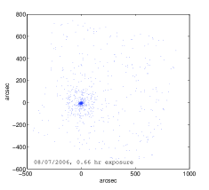
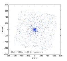
Figure 1: The dust rings seen in the 1st (left, $\approx$31 hr after the burst) and 2nd (right, $\approx$90 hr after the burst) ${\it Swift}$/XRT observations, (energy range 2.5−8.5 keV).

3 Dust scattered x-ray rings

An SGR flare can be considered a special case of a varying source, where the flare is approximately a delta function in time, and the result of an intervening dust screen is a ring expanding with time. For small scattering angles and a single scattering screen, geometry dictates

$$\theta(t)\cong\left[\frac{2c}{d}\frac{\left(1-x\right)}{x}t\right]^{1/2}$$ (1)

where $\theta(t)$ is the measured ring angle with respect to the line of sight, $d$ is the source distance, $x$ is the screen’s location expressed as a fraction of $d$, and $t$ is the time passed since the direct flare observation.

We fit the observations to a model based on Smith & Dwek (1998), with differential scattering cross section as described in Rivera-Ingraham & van Kerkwijk (2010). The original model calculates the halo observed by the scattering of x-rays from a persistent source over a continuous distribution of intervening dust. We are interested in the rings produced by the scattering of an impulsive emission over one or more molecular clouds, namely a discrete distribution of intervening dust. Our configuration is simpler and it allows us to derive an analytic solution. We therefore modify the original derivation by Smith & Dwek (1998) to obtain an analytic expression for the flux in a ring produced by the scattering of a flare on a single thin dust screen, i.e. the scattered flux observed at an angular distance $\theta_{{\rm obs}}(t)$ from the central source, as a function of photon energy. The modification is straight forward and we therefore do not repeat the derivation of Smith & Dwek (1998) here, and just highlight the modifications. Keeping the original notations, we replace the dust distribution along the line of sight with the dust column density across the scattering screen, $N_{\rm dust}$ and the dust grain size distribution with $N_{\rm a}$, such that $N_{\rm dust}=\int N_{\rm a}da$ where $a$ is the radius of the dust grain. We further replace the flux reaching the scatterer, used in the original derivation, by the flare’s total fluence reaching it. In addition, the solid angle which the scattered observed signal occupies, $d\Omega^{\prime}$, is $2\pi\theta(t)d\theta$ where $d\theta$ is the change in the observed angle during the observation time $dt$. Using Equation 1 we find $d\Omega^{\prime}=g\left(x\right)dt$ where $g\left(x\right)=\frac{2\pi c}{d}\frac{\left(1-x\right)}{x}$. The observed scattered flux per photon energy $E$, $F_{E}$ (energy observed in a ring per photons of energy $E$ per unit area per unit time $dt$) is thus:

$$F_{E}\left(\theta_{\rm obs}[t]\right)=S_{E}\frac{g(x)}{(1-x)^{2}}\int_{a_{{\rm min}}}^{a_{{\rm max}}}N_{\rm a}\left(\frac{d\sigma}{d\Omega}\right)da$$ (2)

where $S_{E}$ is the flare’s direct (vs. scattered) observed fluence per photon energy $E$ and $d\sigma(E,a,\theta_{{\rm scat}})/d\Omega$ is the differential scattering cross section of an x-ray with energy $E$ by a dust grain with radius $a$ at an angle $\theta_{{\rm scat}}$.

As scattering angles are small, we substitute $\theta_{{\rm scat}}=\theta_{{\rm obs}}/(1-x)$. For the dust grain size distribution we assume a power-law $N_{\rm a}=Aa^{q}$ where $a_{{\rm min}}\leq a\leq a_{{\rm max}}$ (Mathis et al., 1977). For the differential cross section we use the Gaussian approximation of the Rayleigh-Gans theory, valid for small scattering angles and energies above 1keV, following van de Hulst (1957):

$$\frac{d\sigma(E,a,\theta_{{\rm scat}})}{d\Omega}\cong C_{{\rm dust}}a^{6}\exp\left(-\frac{\theta_{{\rm scat}}^{2}}{2\tilde{\theta}_{{\rm scat}}^{2}}\right)$$ (3)

where $C_{{\rm dust}}$ depends on dust components atomic charge, mass number, density, and scattering factor, while $\tilde{\theta}_{{\rm scat}}$ is given by Mauche & Gorenstein (1986)

$$\tilde{\theta}_{{\rm scat}}\left(a,E\right)=10.4\frac{1}{(E/1\mbox{keV})(a/0.1\mu\mbox{m})}\,{\rm arcmin}$$ (4)

Inserting the cross section and dust grain size distribution we obtain

$$\begin{array}[]{l}F_{E}(\theta_{{\rm obs}},q,\hat{a}_{{\rm max}},\hat{a}_{{\rm min}})=\\ \\ B_{E}\int_{\hat{a}_{{\rm min}}}^{\hat{a}_{{\rm max}}}\hat{a}^{q+6}\exp\left\{-\frac{1}{2}\left(\frac{\theta_{\rm obs}}{10.4^{\prime}}\right)^{2}\left(\frac{\hat{a}}{0.1\mu\mbox{m}}\right)^{2}\left(\frac{E}{1\mbox{keV}}\right)^{2}\right\}d\hat{a}\end{array}$$ (5)

where $\hat{a}\equiv\frac{a}{1-x}$, and

$$B_{E}=S_{E}C_{{\rm dust}}A\frac{2\pi c}{d}(1-x)^{q+6}/x$$ (6)

The differential cross section (Equation 3) implies that a dust grain of size $a$ scatters effectively below a characteristic angle $\tilde{\theta}\left(a\right)$, above which the differential cross section decays rapidly. Thus, for a grain size distribution more gradual than $a^{-7}$, regardless of its exact form, the scattering at an angle $\theta_{\rm scat}$ is dominated by the grain size matching Equation 4,

$$a_{\rm scat}(\theta_{\rm scat},E)\approx\frac{0.1}{(E/1\mbox{keV})(\theta_{\rm scat}/10.4{\rm arcmin})}\mu\mbox{m}$$ (7)

The observed scattered flux can then be approximated as $F_{E}(\theta)\propto N_{\rm a_{\,\rm scat}}a_{\rm scat}^{7}$. If the grain size distribution is limited to the range $a_{{\rm min}}\leq a\leq a_{{\rm max}}$ then at small angles (early time) $a_{\,\rm scat}>a_{{\rm max}}$ and the scattering is dominated by the largest grains, namely it is constant in angle (time) and $F_{E}\propto N_{a_{\rm max}}a_{{\rm max}}^{7}$. At large angles (late time) when $a_{\,\rm scat}<a_{{\rm min}}$ the scattering is dominated by the Gaussian tail of the smallest grains cross-section, and the flux falls exponentially. Therefore, defining $\tilde{\theta}=\left(1-x\right)\tilde{\theta}_{{\rm scat}}$, Equation 5 can be approximated as

$$F_{{\rm E}}(\theta)\propto\left\{\begin{array}[]{ll}const&\theta_{{\rm obs}}\ll\tilde{\theta}\left(a_{{\rm max}}\right)\\ \theta_{{\rm obs}}^{-(q+7)}&\tilde{\theta}\left(a_{{\rm max}}\right)\ll\theta_{{\rm obs}}\ll\tilde{\theta}\left(a_{{\rm min}}\right)\\ \exp\left[-\frac{\theta_{{\rm obs}}^{2}}{\tilde{\theta}^{2}\left(a_{{\rm min}}\right)}\right]&\theta_{{\rm obs}}\gg\tilde{\theta}\left(a_{{\rm min}}\right)\end{array}\right.$$ (8)

It is useful to express this approximation in terms of the flux dependence on time, using Equation 1:

$$F_{{\rm E}}(t)\propto\left\{\begin{array}[]{ll}const&t\ll\tilde{t}\left(a_{{\rm max}}\right)\\ t^{-(q+7)/2}&\tilde{t}\left(a_{{\rm max}}\right)\ll t\ll\tilde{t}\left(a_{{\rm min}}\right)\\ \exp\left[-\frac{t}{\tilde{t}\left(a_{{\rm min}}\right)}\right]&t\gg\tilde{t}\left(a_{{\rm min}}\right)\end{array}\right.$$ (9)

where $\tilde{t}\left(a,E\right)=\frac{d\,x}{2c\left(1-x\right)}\tilde{\theta}^{2}\left(a,E\right)$. These expressions describe three flux regimes − (i) a constant set by scattering over the largest grains. (ii) A power-law decay where the size of the grains that dominate the scattering vary with time and (iii) an exponential decay set by the scattering cross section of the smallest grains. Therefore, observing the evolution of $F_{E}$ with time is a direct probe of the dust grain size distribution. $a_{{\rm max}}$ is probed by observations covering the time of transition between the constant and the power-law regime, while the index $q$ is obtained by power-law regime observations. Probing $a_{{\rm min}}$ requires a burst bright enough for the scattered signal to overcome the background at the low end of the power-law regime.

We note that Equation 10 in Draine (2003), which is an analytical approximation for the differential scattering cross section describing his model of x-ray scattering by dust, can be closely matched by the above scattering model by choosing $a_{{\rm max}}=0.33\,\mu\mbox{m}$ and $q=-3$, which are typical values for ISM dust.

4 Analysis & Results

To obtain our two objectives − constraining the distance to SGR 1806−20 and the properties of the dust in the intervening molecular clouds, we take two different approaches in analyzing the XRT observations. First (Section 4.1), we assume positions and visual extinctions of molecular clouds along the line of sight based on CE04 in order to get an estimate of the distance to SGR 1806−20. We test the dependence of this analysis on a dust scattering model and find it to be negligible. Therefore our conclusion is based on the accuracy of CE04 clouds distribution, and is mainly limited by the XRT resolution and sensitivity.

In the second (Section 4.2) we relax our assumptions regarding the distance to the scattering clouds, and motivated by observations we assume a single predominant scattering screen. We keep the location of this screen a free parameter, and use Equation 5 to put simultaneous constraints on both the dust screen location and the dust properties, using a full data set including both spectral and temporal flux evolution. The results of this analysis are limited mainly by the delay of the first observation and by the sensitivity of the XRT detector.

4.1 Distance estimate based on known molecular clouds along the line of sight

Equation 2 expresses the observed scattered flux as a function of: (1) The scatterer’s location relative to the source (i.e., $x$) and (2) Properties of the scattering dust. Therefore, if the location of the scatterers and the properties of the dust are known, one can extract the distance to the source. In fact, as we show here, it is enough to know the location of the dust screens along the line of sight and their dust column densities to put strong constraints on the source distance, even if the grain size distribution, $N_{a}$ is not well known. CE04 provide the locations of the scattering clouds along the line of sight to SGR 1806−20, as well as their optical extinction $A_{V}$, which indicate on their dust column densities. Using this data we calculate the scattered flux radial profile for different locations of the source. We then compare these “synthetic” profiles with the observed profiles and use the best fit profile to infer the distance.

Table 2 lists properties of the molecular clouds along the line of sight, adapted from Table 1 of CE04. Following radial velocity measurements, each cloud has two distance solutions and was therefore attributed with a near distance and a far distance, as well as optical extinction $A_{V}$. For eight clouds CE04 ruled out one of these distances due to additional considerations. We assume that the $A_{V}$ given for each cloud is proportional to its share of the clouds’ total dust column density (i.e. $A_{V}\propto A$ in Equation 6). Equipped with the clouds’ positions and dust shares, we assume a single dust grain size distribution across all clouds and set $a_{{\rm max}}=0.3\,\mu\mbox{m}$, $a_{{\rm min}}=0\,\mu\mbox{m}$, $q=-3$. Assuming a source distance we use Equations 1 and 5 to calculate the scattered flux from each of the intervening clouds and construct a synthetic flux radial profile at any given time and energy band. In order to compare the profile calculated using Equations 1 and 5 to the observations, it must be smeared by the PSF, the exposure duration and the width of the scattering clouds. We therefore introduce the ${\it Swift}$/XRT PSF function (Moretti et al., 2005), and we account for the observations actual exposure durations to widen the profile beyond the PSF effect. Assuming a typical molecular cloud width of $\sim 100\,{\rm pc}$, the consequent smear is negligible. We repeat this calculation for an SGR 1806−20 distance that vary in the range 5−25 kpc with a 0.1 kpc resolution. Note that the synthetic profiles are calculated up to a normalization factor per energy band, accounting for the unknown direct fluence from the source $S_{{\rm E}}$, as well as both $C_{\rm dust}$ and the constant of proportionality in $A\propto A_{V}$.

Table 2: Molecular clouds along the line of sight to LBV 1806−20, taken from CE04. The bottom three clouds, lacking unambiguous distance determinations, are quoted with both near/far distances ($1\sigma$ errors). CE04 do not determine whether the three last clouds in this table are in front or behind the Galactic center, allowing two distances to each cloud. In the text we refer to all three clouds being in front of the Galactic center as the ‘near’ configuration, while all three clouds being at their far distance is the ‘far’ configuration.

Name	$A_{V}$	Distance
	[magnitude]	[kpc]
MC-16	8.6$\pm$1.7	4.5$\pm$0.3
MC4	3.9$\pm$0.8	0.2$\pm 0.5$
MC13A	10.0$\pm$2.0	15.1$\pm$0.9
MC13B	3.0$\pm$0.6	4.5$\pm$0.3
MC24	5.6$\pm$1.1	3.0$\pm$0.5
MC30	0.8$\pm$0.2	3.5$\pm$0.35
MC38	1.1$\pm$0.2	4.2$\pm$0.3
MC44	1.6$\pm$0.3	4.5$\pm$0.3
MC73	6.0$\pm$1.2	5.7/11.0$\pm$0.15
MC87	1.4$\pm$0.3	6.1/10.6$\pm$0.15
MC94	0.5$\pm$0.1	6.2/10.5$\pm$0.15

The actual observed signal contains two additional features beyond the dust scattered flux, and we therefore model the observed radial flux profile as a sum of the three following contributions: (a) the synthetic profile of the dust scattered signal, calculated as described above (b) the measured background profile, and (c) the halo around the SGR described in Section 2. Therefore, our model contains the following free parameters: the halo amplitude and power-law per observed profile, the normalization factor of the scattered signal per energy band, and the SGR distance.

We compare this model with the observed profiles from the first two epochs in Table 1, where the observed dust scattered ring is most evident, with each epoch split into two energy bands. For each distance we use a $\chi^{2}$ fit to find the halo amplitude and power-law per observed profile, and the normalization factor per energy band. We then calculate $\chi^{2}$ as a function of distance and choose the distance yielding the overall minimal $\chi^{2}$ as the best fit distance.

Three of the clouds lack an unambiguous distance determination and have instead both a near and a far distance estimates, similar for all three clouds. To account for this uncertainty we prepare two sets of scattered signal profiles as a function of SGR distance, one with all three clouds set at their ’near’ position, the other with all three at their ’far’ position, and repeat the above procedure for both sets. We verify that other combinations, where some of the clouds are at an opposite location, result in intermediate SGR locations and therefore the ’far’ and ’near’ configurations bracket the constraints on the location of SGR 1806−20.

In order to estimate the distance error we use Monte Carlo simulations (following the prescription in Press et al. 1986). For each Monte Carlo realization we generate a pseudo binned radial profile by drawing the “observed” radial bins photon counts from a Poisson distribution around the best fit radial profile. We further prepare synthetic scattered profiles per SGR distance by drawing clouds’ positions and optical extinctions (from Table 2) assuming an approximately normal distribution for both. We repeat the fitting procedure described above for each of 10,000 Monte Carlo realizations and thus obtain the probability distribution of the SGR distance (see Figure 2).

To account for the dependence of the distance on the dust grain size distribution we run the complete procedure described above for nine different parameter choices of Equation 5, with the permutations of $a_{{\rm max}}=0.15,0.3,0.6\,\mu\mbox{m}$ and $q=-3.5,-3,-2.5$. We find the best fit distance scatter due to the model choice to be smaller than the scatter due to the errors of the binned signal and of the clouds’ positions and opacities (a scatter of $\sim 1$ kpc between the two extreme model parameter choices, compared to $\sim 3.5$ kpc $\left(1\sigma\right)$ scatter due to the errors). We therefore set the intermediate values of $a_{{\rm max}}=0.3\,\mu\mbox{m}$ and $q=-3$ as our model parameters for the analysis. In Section 4.2 we measure $q$ and find a lower limit for $a_{\rm max}$, which are consistent with the parameters we choose for this analysis, and which errors are consistent with the range we use for this parameter independency check. The absence of a measured upper limit for $a_{\rm max}$ has no influence on this analysis since the dominant clouds fall within the power-law regime (see Equation 4) for any $a_{\rm max}$ bigger than the value chosen here.

The effect of the SGR position on the scattered signal and on the fit quality is demonstrated in Figure 3. For an SGR at 16 kpc, the clouds concentrations at 4.5 and 6 kpc nearly merge, overlapping with the measured signal, while the 3 kpc clouds are negligible. In contrast, with the SGR at 6 kpc the clouds concentrations are more separated, with the dominant 4.5 kpc cloud and the measured signal largely unsynchronized. For the ’near’ configuration, the best fit distance is $16{}_{-3.8}^{+2.6}$ kpc (90% confidence), with $\chi^{2}/{\rm dof}=43.3/47$. For the ’far’ configuration, best fit distance is $11.9_{-2.5}^{+1.6}$ kpc (90% confidence) with $\chi^{2}/{\rm dof}=45.9/47$. Since the goodness of fit for both configurations is similar we use their combination to set conservative limits, with a lower limit of $9.4$ kpc and an upper limits of $18.6$ kpc on the distance to SGR 1806−20 at a 90% confidence level.

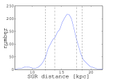
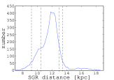
Figure 2: The distributions of the distance to SGR 1806−20 obtained by Monte Carlo simulations, with 68% and 90% confidence limits marked. The left (right) distribution matches the ’near’ (’far’) clouds configuration, where the three clouds with ambiguous locations are fixed at their near (far) locations (see Table 2). The best fit distance is $16{}_{-3.8}^{+2.6}$ kpc for the ’near’ configuration and $11.9_{-2.5}^{+1.6}$ kpc for the ’far’ configuration (90% confidence).

We note that taking the main bulk of the dust along the line of sight according to CE04, concentrated at 4.5 kpc, and substituting in Equation 1 with our observed ring’s $\theta$ and $t$, results in a distance of 15 kpc for SGR 1806−20. Our above analysis wraps this crude estimation with the confidence limits permitted by the XRT observations and the CE04 errors.

The weakest link of our analysis is the accuracy of the clouds’ locations as reported in CE04. As an example, Figer et al. (2004) suggested, based on a different method for measuring the radial velocity, a distance of 11.8 kpc (vs. 15.1$\pm$0.9 of CE04) to cloud MC13A. Although this cloud has minor influence on our analysis, the discrepancy in this measurement demonstrates the limitation of our method. However, the goodness of fit we obtain, $\chi^{2}/\mbox{dof}\approx 1$, provides a consistency check for the CE04 clouds distribution along the line of sight. In Section 5 we argue that future post-burst observations could resolve the location of a few individual clouds. This would potentially permit an SGR distance estimate that depends, independently, on the location of each of the resolved clouds, thereby resulting in a more robust and accurate distance measurement for this SGR.

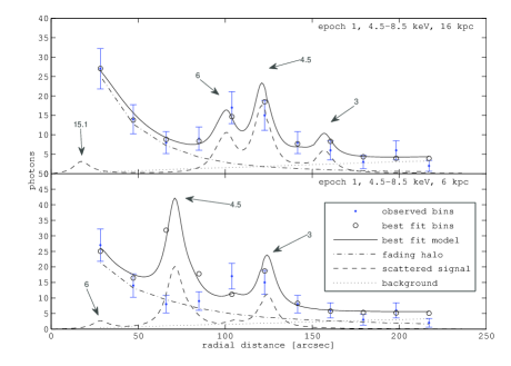
Figure 3: A comparison between the best fit $\chi^{2}$ obtained for SGR 1806−20 located at 6 kpc vs. 16 kpc, with clouds at the ’near’ clouds configuration (see Table 2). Circles mark the best fit model binnned photon counts while dots with error bars (Poisson, $1\sigma)$ mark the measured bin photon counts. Arrows indicate the positions in kpc of the main clouds concentrations corresponding to each peak. An SGR distance of 16 kpc evidently provides a good fit to the data, while a distance of 6 kpc is ruled out at a $>3\sigma$ level. Model components: Dotted line is background, dotted-dashed is the fading halo, dashed is the calculated signal profile, continuous line is sum of the three components of the best fit model.

4.2 Constraints on dust properties

Here we assume a single predominant dust screen at an unknown a-priori location, thus dropping our previous rely on CE04 results. This assumption is motivated by the fact that the XRT observations show a single ring. Fitting the observed radial profile fluxes and photon energies using Equation 5, we obtain best fit values for $\hat{a}_{{\rm max}}$, $q$ and $B(E)$. Since $\hat{a}_{{\rm max}}=a_{{\rm max}}/\left(1-x\right)$ the fit results in a joint constraint on $a_{{\rm max}}$ and $x$. The model we use assumes a power-law grain size distribution $N_{\rm a}\propto a^{q}$ with grain size $a_{{\rm min}}<a<a_{{\rm max}}$, leading to the three scattered flux regimes described in Equation 8. Thus, constraining $q$ requires observations at epochs or angles within the power-law regime, while constraining $\hat{a}_{{\rm max}}$ requires the further inclusion of earlier observations, towards the constant flux asymptote.

Fitting the observations to the dust model is done in two steps. First we find the integrated scattered signal flux within the ring and its associated flux probability distribution (from simulations) per epoch (for the four epoches in Table 1) per energy band by fitting the observed data to a model. Then we use these fluxes as a function of epoch and energy, and their probability distributions, to obtain best fit values for $\hat{a}_{{\rm max}}$, $q$ and $B(E)$ by means of a Maximum likelihood fit using Equation 5.

We model the dust scattered signal as a Gaussian profile, thus accounting for ${\it Swift}$ PSF and exposure duration effect, assuming that the effect of the clouds’ width is negligible. In order to calculate the scattered signal net flux per energy band per epoch, we fit each observed radial profile to a model composed of the following three components: (a) the Gaussian profile representing the scattered signal (b) the measured background profile, and (c) the halo around the SGR described in Section 2. The contribution of each component to each bin is weighted according to the bin’s average exposure time due to the exposure maps. We run a minimum $\chi^{2}$ fit with the fading halo amplitude and power, and the Gaussian amplitude and width as the free parameters. For the first observation we also fit for the radius of the Gaussian center and obtain $\theta=119\pm 5^{\prime\prime}\,(2\sigma)$. We fix the ring location of the other observations using $\theta\left(t\right)\propto\sqrt{t}$ (Equation 1). Figure 4 shows the best fit model for the first two epochs. The best fit Gaussian area translates to the photon count per second related to the scattered signal, which we convert to flux using NASA’s HEASARC web based tool WebPIMMS.

We find probability distributions of each ring’s integrated flux by Monte Carlo simulations. The best fit radial profile from the $\chi^{2}$ fit is used as the base data set for preparing (assuming Poisson distribution for the bins photon count) 5000 binned profile realizations. Collecting the best fit flux of each realization we compile the flux probability distribution.

These distributions are then used as the input for a Maximum Likelihood fit, where we find the best fit values for $\hat{a}_{{\rm max}}$ and $q$, along with two normalization factors $B_{E}$, one per energy band. For a given set of parameters $\hat{a}_{{\rm max}},q$ and $B(E)$ we use Equation 5 to calculate the flux at each observation epoch and energy band. We then evaluate the likelihood of this set using the measured flux distribution. The set of parameter values which yields the highest product of likelihoods for all epochs and energy bands is the best fit. Figure 5 shows the $1\sigma$ bars of the flux distributions, and the corresponding best fit model.

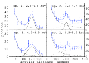
Figure 4: $\chi^{2}$ fits for the first two epochs in the two energy bands. The dotted line is background, dotted-dashed is the fading halo, bottom continuous line is the scattered signal Gaussian and top line is the sum of the three components. Dots with error bars (Poisson, $1\sigma$) are the binned measured photon counts. The best fit Gaussian area translates to the flux per epoch and energy band (Table 3), flux errors distribution are found using Monte Carlo simulations (see text).

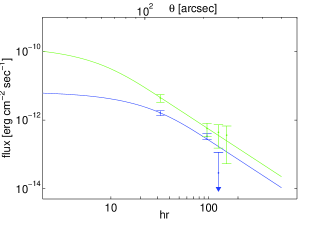
Figure 5: Maximum likelihood best fit model (Equation 5). Lower line and accompanying dots and error bars (Table 3) are the 2.5−4.5 keV band. The best fit result for the power-law index $q$ is $-3.3_{-0.7}^{+0.6}$ ($1\sigma$), with errors determined from Monte Carlo simulations. The best fit result for $\hat{a}_{{\rm max}}=a_{{\rm max}}/(1-x)$ is $0.33\,\mu\mbox{m}$. Since the first observation is almost completely within the flux power-law regime (see Equation 8), we can not set an upper limit for $\hat{a}_{{\rm max}}$. The $2\sigma$ lower limit is $0.21\,\mu\mbox{m}$ (see Figure 6).

Estimation of the confidence limits of these parameters is calculated by Monte Carlo simulations. For each Monte Carlo run we generate a realization of the fluxes in Table 3, with the ring’s integrated flux values drawn from the actual best fit distribution in Table 3. The errors around the drawn flux values are taken to be the same as the original errors in Table 3. We fit 5000 Monte Carlo realizations for $\hat{a}_{{\rm max}},q$ and $B(E)$, thus obtaining the probability distribution of these parameters.

Table 3: Best fit ring’s integrated fluxes used for the maximum likelihood fit

Epoch	Time since burst	Energy band	Flux	$\chi^{2}$/dof
	[hr]	[keV]	[$\mbox{erg}\,\mbox{cm}^{-2}\mbox{s}^{-1}$]
1	30.8	2.5−4.5	$1.63\pm 0.27\times 10^{-12}$	2.95/4
1	30.8	4.5−8.5	$4.45\pm 1.13\times 10^{-12}$	2.00/5
2	93.5	2.5−4.5	$3.39\pm 0.71\times 10^{-13}$	6.15/15
2	93.5	4.5−8.5	$5.73\pm 2.45\times 10^{-13}$	17.25/15
3	121.1	2.5−4.5	$2.88\pm 8.70\times 10^{-14}$	7.59/11
3	121.1	4.5−8.5	$4.43\pm 2.92\times 10^{-13}$	13.31/11
4	147.6	4.5−8.5	$3.64\pm 3.12\times 10^{-13}$	16.83/11

Fluxes used for the maximum likelihood fit, with $1\sigma$ errors and $\chi^{2}$ values, are listed in Table 1. The best fit result for $q$ is $-3.3_{-0.7}^{+0.6}$ ($1\sigma$), consistent with the commonly cited $-3.5$ from Mathis et al. (1977) and with an implicit $-3$ of Draine (2003). The best fit result for $\hat{a}_{{\rm max}}$ is $0.33\,\mu\mbox{m}$. As indicated by the likelihood contours of $q$ and $\hat{a}_{{\rm max}}$ shown in Figure 6, we are unable to constrain $\hat{a}_{{\rm max}}$ from above, which is the result of the earliest observation being too adjacent to the power-law asymptote regime (see Figure 5). We thus find only a lower limit of $0.21\,\mu\mbox{m}$ ($2\sigma$) for $\hat{a}_{{\rm max}}$.

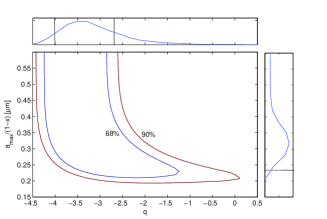
Figure 6: 68% and 90% likelihood contours of $q$ and $\hat{a}_{{\rm max}}$ as determined from the Monte Carlo simulations. Note the lack of an upper limit for $\hat{a}_{{\rm max}}$. The marginalized distribution of each parameter are shown above ($q$) and to the right ($\hat{a}_{{\rm max}}$). The lines mark the 68% confidence limits for each single parameter, based on an integration of the probabilities for $\hat{a}_{{\rm max}}\leq 3\mu\mbox{m}$.

In our fit we constrain $\hat{a}_{{\rm max}}$, which is a combination of $a_{{\rm max}}$ and $x$ ($\hat{a}_{{\rm max}}\equiv\frac{a_{{\rm max}}}{1-x}$). In order to learn further about either $x$ or $a_{{\rm max}}$ one needs to have prior knowledge of either $a_{{\rm max}}$ or $x$, respectively. Since $\theta\left(t\right)$ is known, a measurement of $x$ will provide an SGR distance estimate that is independent of our previous analysis. However, prior constraints on the distance to SGR 1806−20, 6−15 kpc (Section 1), translate, together with the locations of the ring, to $0.30<x<0.51$ (Equation 1). Therefore, improving these constraints on $x$ requires constraints on both $\hat{a}_{{\rm max}}$ and $a_{{\rm max}}$ that are better than 25%. The uncertainty in the value of $\hat{a}_{{\rm max}}$ in the diffuse ISM is larger, while its value in molecular clouds is practically unknown. Therefore, our measured $\hat{a}_{{\rm max}}$, and even an ideal errorless $\hat{a}_{{\rm max}}$, are useless for improving the constraints on the distance to SGR 1806−20. This conclusion is similar to that of Tiengo et al. (2010), which find that the distance to the X-ray pulsar 1E1547.0–5408 cannot be conclusively determined due to the uncertainty in the dust properties, although they obtained superb data.

In the case of SGR 1806-20, however, there are robust (although rather loose) limits on its distance. Thus, the prior constraints on $x$ can be used to efficiently constrain $a_{{\rm max}}$, which is of special interest in our case of molecular clouds. The robust constraint of $d>6$ kpc for the SGR’s distance (Cameron et al., 2005) matches to $x<0.51$, which translates to $a_{{\rm max}}>0.1\,\mu\mbox{m}$ ($2\sigma$).

The best fit results for the normalization factors are $B(2.5-4.5{\rm keV})=2.89_{-0.81}^{+0.86}\times 10^{-13}$ $\mbox{erg}\,\mbox{cm}^{-2}\,\mbox{s}^{-1}\,\mbox{asec}^{-2}$, $B(4.5-8.5{\rm keV})=6.10_{-1.21}^{+1.27}\times 10^{-12}$ $\mbox{erg}\,\mbox{cm}^{-2}\,\mbox{s}^{-1}\,\mbox{asec}^{-2}$. As a consistency check, we use the ratio between the two normalization constants to find the Hydrogen column density towards SGR 1806−20. The normalization constant depends on photon energy through $S_{E}$, the direct observed fluence. Given the source spectrum and the x-ray extinction cross section per H nucleon per energy $\sigma(E)$, $N_{H}$ can be extracted using $S_{E}\propto\exp\{-\sigma(E)N_{H}\}$. Assuming the x-ray extinction is mainly dust driven, we take the x-ray extinction cross section per H nucleon due to dust for each energy band from Draine (2003) (assuming $R_{V}=3.1$). For the burst x-ray spectrum at our energy bands we follow Feroci et al. (2004) and Olive et al. (2003) in adopting a double black body spectrum instead of the OTTB spectrum commonly used to describe SGR bursts in the range $20-200\,{\rm keV}$ (e.g. Golenetskii et al. 2005). Using the average double black body spectrum of $kT_{1}=3.4,\,kT_{2}=9.3,\,L_{1}/L_{2}=0.85$ from Feroci et al. (2004) with our best fit ratio we get $N_{H}=9.64_{-4.0}^{+2.8}\times 10^{22}\mbox{cm}^{-2}$, consistent with Sonobe et al. (1994).

Reversing the last procedure we find the normalizations ratio between the 2.5−4.5 keV band and the 0.5−2.5 keV band, which we did not use due to lack of signal, to be 1000:1, explaining the lack of signal beyond the background noise in the 0.5−2.5 keV energy band.

5 Future SGRs observations

The accuracy of the derived distance to SGR 1806−20 and the properties of the dust along the line of sight are restricted by large error bars due to the weak signal and low resolution of the ${\it Swift}$/XRT, and by the long delay between the burst and the first echo observation. Nevertheless, our analyses demonstrate the wealth of information that can be extracted from observing dust scattered x-ray echoes of bursts. Encouraged by these results, we provide guidelines for optimal future observations of magnetar bursts, showing that improved observations’ timing, resolution and sensitivity would yield far better constraints on both the distance to an SGR and the properties of the intervening dust.

In order to evaluate the expected angular scattered width of the ring we compare the effects of clouds width, exposure duration and PSF. Substituting an SGR distance of 15 kpc and $x=0.3$ (i.e. main cloud at 4.5 kpc) in Equation 1 we get a spread of roughly 1^′′ for an assumed typical cloud width of 100 pc, and a spread of $\Delta\theta=0.36^{\prime\prime}\left(t_{{\rm start}}^{\frac{1}{2}}-t_{{\rm end}}^{\frac{1}{2}}\right)$ due to exposure duration (where $t$ is the time passed in seconds since the burst direct observation). This yields a width of $\sim$1^′′ for the first XRT epoch, at a delay of 30 hours and duration of 40 minutes, due to the non-PSF effects. Thus the width is practically set by the PSF of the telescope, with $\sim$20^′′ for ${\it Swift}$/XRT vs. 1^′′ for Chandra.

Effective constraining of $a_{{\rm max}}$ requires observations earlier than 30 hours after the burst, and such a response time is suitable for ${\it Swift}$/XRT. With a stronger scattered signal and a sharper decay of the King component for earlier observations, resolving the scattered signal from the source should be possible for a $\sim$1 hr observation taken 12 hours after the burst ($\theta_{{\rm obs}}=75^{\prime\prime}$). Since observations should also cover the scattered flux power-law regime, the burst fluence should be similar or larger than the 2006 August 6 burst.

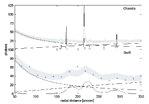
Figure 7: A comparison of the best fit photon counts for the second epoch 2.5−4.5 keV band with SGR at 16 kpc, ${\it Swift}$ vs. Chandra. Based on a Chandra 4-fold signal and 3^′′ resolution. Contributions of clouds scattered signal, background and fading halo are shown as continuous lines. Poisson $1\sigma$ confidence limits for the best fit photon counts are marked as gray filled area. ${\it Swift}$ actual measured photon counts are marked in circles.

Chandra observation can be obtained with a response time of a few days. The improved resolution and collection area of Chandra could significantly reduce errors and improve statistics. Chandra also enables a continuous observation due to its high orbit, thus minimizing the spread due to exposure duration. A resolution of 2^′′−3^′′ (accounting for PSF, exposure duration and cloud width) and a signal roughly four times that of ${\it Swift}$ should improve the signal to noise ratio, and enable resolving the location of individual clouds along the line of sight. Each of the resolved clouds will provide an independent constraint on the SGR distance. This will provide a more accurate and, more importantly, a more robust distance estimate. In Figure 7 we illustrate the advantages of using Chandra, comparing what Chandra would have seen at the second XRT epoch to the actual ${\it Swift}$ observation.

The burst energy determines the proper time for the last effective observation. A delay of 30 hours, equivalent to $\theta=120^{\prime\prime}$, is located within the power-law regime flux decay (Equation 8), as seen in Figure 5. Using our $q=-3.3$, combined with our measured scattered flux, we get

$$F_{{\rm scat}}=F_{0}\,\frac{\Phi}{\Phi_{\rm\,August\,6,\,2006}}\left(\frac{t_{{\rm delay}}}{30\,\mbox{hr}}\right)^{-1.85}$$ (10)

where $F_{0}(2.5-4.5\,{\rm keV})=1.63\times 10^{-12}{\rm\,erg\,cm^{-2}\,s^{-1}}$ and $F_{0}(2.5-4.5\,{\rm keV})=4.45\times 10^{-12}{\rm\,erg\,cm^{-2}\,s^{-1}}$ are the fluxes from table 3. The equation is valid for $t_{{\rm delay}}\eqslantgtr 30$ hours (power-law regime). We calibrate the background photon count by the total background photon count measured for ${\it Swift}$ (e.g. $0.14\,{\rm ph\,s^{-1}}$ for $2.5-4.5\,{\rm keV}$), with the background per radial bin piling up as $\theta\propto\sqrt{t}$. By requiring the bin which contains the largest fraction $f\leq 1$ of the scattered signal to be $N_{\sigma}$ times larger than the background error we get a rough estimation of the maximum delay for an effective observation:

$$\begin{array}[]{l}t=\\ t_{0}\left(\frac{\Phi}{\Phi_{\rm\,August\,6,\,2006}}\frac{5}{N_{\sigma}}f\sqrt{\frac{10^{\prime\prime}}{\mbox{bin width}}\frac{A_{{\rm eff}}}{A_{{\rm eff}}^{{\rm Swift}}}\frac{\Delta t}{1\,\rm hr}}\right)^{0.48}\end{array}$$ (11)

where $t_{0}(2.5-4.5\,{\rm keV})=135\,{\rm hr}$ and $t_{0}(4.5-8.5\,{\rm keV})=120\,{\rm hr}$, $A_{\rm eff}$ is the detector’s effective area for the chosen energy band, and $\Delta t$ is the observation’s exposure time in hours.

For the ${\it Swift}$ case at $2.5-4.5\,{\rm keV}$ we get a $>5\sigma$ detection for the first observation, at t=30 hr, and a $\sim 5\sigma$ detection for the t=100 hr second observation. A Chandra $A_{{\rm eff}}\approx 4A_{{\rm eff}}^{{\rm Swift}}$, $\Delta t=5\,$hr (for the latest observation), a bin width of 3^′′ and $f\approx 1$ permits a $5\sigma$ detection as long as 370 hr after a burst of the same fluence, thus probing dust grains down to a size of $\sim 0.022\,\mu\mbox{m}$ (vs. $\sim 0.035\,\mu\mbox{m}$ in our case). Alternatively, a Chandra observation of $\Delta t=3\,$hr after 100 hr can yield a $5\sigma$ detection for a burst of a fluence ten times weaker than that of 2006 August 6. Such SGR bursts are more common, offering more opportunities for observations.

Equations 10 and 11 quote the fluence of the 2006 August 6 burst. The measured event fluence at the range 20−200 keV is $\Phi=2.4\times 10^{-4}\mbox{erg}\cdot\mbox{cm}^{-2}$ (Golenetskii et al., 2006). We assume, at least for minor/intermediate bursts, a similar spectrum across different energy outputs (e.g. Olive et al., 2003; Feroci et al., 2004). Hence, for events which fluence is given at 20−200 keV, one should substitute the above cited fluence along with the new event fluence. For events where the band fluence (e.g. $2.5-4.5\,\mbox{keV}$) is more accessible, or events for which the similar spectrum assumption does not necessarily hold (e.g. giant flares), we supply an estimate of the 2006 August 6 burst fluence at the $2.5-4.5\,\mbox{keV}$ and the $4.5-8.5\,\mbox{keV}$ energy bands. Olive et al. (2004), Feroci et al. (2004), Nakagawa et al. (2007) and Israel et al. (2008) obtain satisfying fits for the spectra of minor/intermediate SGR bursts using models composed of two blackbody components, a harder $kT\approx 9-10$ one and a softer $kT\approx 3-4$ one. Israel et al. (2008) compared three of the cited works and found the bolometric luminosities of the two components to be similar, with a possible saturation of the soft component above $10^{41}\,{\rm erg\,s^{-1}}$. We adopt an equal luminosity for both components. Calibrating all the cited models with the SGR fluence per keV at $kT=20$ (derived from the total measured fluence and an OTTB spectrum of $kT=20$ keV over the range of 20$-$200 keV), we calculate the band fluence according to the blackbody temperatures of each cited model, and estimate the fluence as the geometric mean of the two extreme model results, obtaining $\Phi_{2.5-4.5}=1.0^{+0.9}_{-0.4}\times 10^{-6}\,{\rm erg\,cm^{-2}}$ and $\Phi_{4.5-8.5}=8.3^{+5.0}_{-3.2}\times 10^{-6}\,{\rm erg\,cm^{-2}}$. These values can be used for equations 10 and 11 along with the respective band fluence of a new event, regardless of the event’s spectrum.

A burst brighter than the one we analyzed should enable probing smaller dust grains and even, if bright enough, allow the determination of $a_{{\rm min}}$, the lower cutoff of the dust grain size distribution. The launch of NuSTAR next year may provide an opportunity to constrain $a_{{\rm min}}$ by observing echoes from an intermediate burst, since for a given $a_{{\rm min}}$ the transition time from the power-law regime to the exponential decay regime is proportional to $\theta^{2}$ and therefore to $E^{-2}$ (Equation 4). NuSTAR has a sensitivity range of $5-80\,{\rm keV}$ and a larger effective area compared to Chandra (for $E<35\,{\rm keV}$ ). In addition, the signal to noise at higher energies should improve due to the spectrum of SGR bursts and to the decrease in the background level. On the other hand, NuSTAR’s relatively low resolution of $43^{\prime\prime}$ will dilute the signal. Taking it all into account, NuSTAR should be able to follow hard x-ray echoes from intermediate bursts for a few days after the burst, thus probing much smaller grains, and potentially identifying $a_{{\rm min}}$.

Generally, x-ray echoes observations taken during different bursts of the same SGR can be combined to improve signal to noise ratio and thus improve the constraints discussed in this work.

6 Conclusions

We used ${\it Swift}$/XRT observations following an intermediate burst of SGR 1806−20 to constrain the distance to the SGR and to find the first x-ray echo constraints on molecular clouds’ dust properties. Based on the molecular clouds’ properties along the line of sight found by CE04 and the observed echoes of the burst we constrain the distance with a lower limit of $9.4$ kpc and an upper limits of $18.6$ kpc at a 90% confidence level. This upper limit can be considered the first direct upper limit set for the distance to the SGR, as the upper limit set by Cameron et al. (2005) is questionable, and other distance estimates are based on association rather than measured emission from the source. Our distance constraints favor an energy output of $\sim 10^{46}\,$erg s^-1 for the 2004 giant flare of SGR 1806−20, leaving Galactic vs. extragalactic giant bursts rates possible tension and the lack of post-burst emission features changes in SGR 1806−20 as open issues.

We introduce the use of observations of dust x-ray echoes for probing the dust properties of molecular clouds. Fitting the spectral and temporal signal evolution using a dust scattering model with an assumed power-law dust grain size distribution we find a power-law index of $q=-3.3_{-0.7}^{+0.6}$ ($1\sigma$) and that the dust maximal grain size $a_{{\rm max}}>0.1\,\mu\mbox{m}$ ($2\sigma$). These results are of special interest since the dust along the line of sight to SGR 1806−20 resides in molecular clouds, which dust properties have been poorly explored. The constraints we got, imply that the dust grain size distribution in molecular clouds may be similar to the one found in diffused ISM (e.g. Mathis et al. 1977).

The wealth of data obtained using ${\it Swift}$/XRT encourage us to suggest the use of future x-ray echoes observations. For an intermediate SGR 1806−20 burst, a ${\it Swift}$ observation starting half a day after the burst and a Chandra observation a few days after the burst should yield superior dust grain size distribution characterization and SGR distance constraints, respectively. A Chandra observation should enable, in addition, a quality mapping of clouds’ locations along the line of sight. NuSTAR, planned to be launched next year, could potentially probe $a_{{\rm min}}$, the minimal dust grain size.

The authors would like to thank Bruce Draine, Eli Dwek, Derek Fox and Amiel Sternberg for helpful discussions. Special thanks to Chryssa Kouveliotou for helpful comments and careful reading of the manuscript. This work was partially supported by the Israel Science Foundation (grant No. 174/08) and by an IRG grant. EOO is supported by an Einstein fellowship and NASA grants.

References

- Bibby et al. (2008) Bibby J. L., Crowther P. A., Furness J. P., Clark J. S., 2008, MNRAS , 386, L23
- Brand & Blitz (1993) Brand J., Blitz L., 1993, A&A , 275, 67
- Burrows et al. (2005) Burrows D. N., Hill J. E., Nousek J. A., Kennea J. A., Wells A., Osborne J. P., Abbey A. F., Beardmore A., Mukerjee K., Short A. D. T., Chincarini G., Campana S., Citterio O., Moretti A., Pagani C., Tagliaferri G., Giommi P., Capalbi M., Tamburelli F., Angelini L., Cusumano G., Bräuninger H. W., Burkert W., Hartner G. D., 2005, Space Sci. Rev. , 120, 165
- Butler & Tan (2009) Butler M. J., Tan J. C., 2009, ApJ , 696, 484
- Cameron et al. (2005) Cameron P. B., Chandra P., Ray A., Kulkarni S. R., Frail D. A., Wieringa M. H., Nakar E., Phinney E. S., Miyazaki A., Tsuboi M., Okumura S., Kawai N., Menten K. M., Bertoldi F., 2005, Nature , 434, 1112
- Carrasco et al. (1973) Carrasco L., Strom S. E., Strom K. M., 1973, ApJ , 182, 95
- Chiar et al. (2007) Chiar J. E., Ennico K., Pendleton Y. J., Boogert A. C. A., Greene T., Knez C., Lada C., Roellig T., Tielens A. G. G. M., Werner M., Whittet D. C. B., 2007, ApJL , 666, L73
- Corbel & Eikenberry (2004) Corbel S., Eikenberry S. S., 2004, A&A , 419, 191
- Draine (2003) Draine B. T., 2003, ApJ , 598, 1026
- Duncan & Thompson (1992) Duncan R. C., Thompson C., 1992, ApJL , 392, L9
- Esposito et al. (2007) Esposito P., Mereghetti S., Tiengo A., Zane S., Turolla R., Götz D., Rea N., Kawai N., Ueno M., Israel G. L., Stella L., Feroci M., 2007, A&A , 476, 321
- Feng & Fox (2010) Feng L., Fox D. B., 2010, MNRAS , 404, 1018
- Feroci et al. (2004) Feroci M., Caliandro G. A., Massaro E., Mereghetti S., Woods P. M., 2004, ApJ , 612, 408
- Figer et al. (2005) Figer D. F., Najarro F., Geballe T. R., Blum R. D., Kudritzki R. P., 2005, ApJL , 622, L49
- Figer et al. (2004) Figer D. F., Najarro F., Kudritzki R. P., 2004, ApJL , 610, L109
- Goad et al. (2006) Goad M. R., Page K. L., Godet O., O’Brien P. T., Vaughan S., Hurley K., 2006, GRB Coordinates Network, 5438, 1
- Goldsmith et al. (1997) Goldsmith P. F., Bergin E. A., Lis D. C., 1997, ApJ , 491, 615
- Golenetskii et al. (2005) Golenetskii S., Aptekar R., Mazets E., Pal’Shin V., Frederiks D., Cline T., Barthelmy S., Cummings J., Gehrels N., Krimm H., 2005, GRB Coordinates Network, 4312, 1
- Golenetskii et al. (2006) Golenetskii S., Frederiks D., Pal’Shin V., Aptekar R., Cline T., Mazets E., 2006, GRB Coordinates Network, 5426, 1
- Göğüş et al. (2004) Göğüş E., Kouveliotou C., Woods P. M., Finger M. H., van der Klis M., 2004, Nuclear Physics B Proceedings Supplements, 132, 604
- Hurley et al. (2006a) Hurley K., Barthelmy S., Cummings J., Gehrels N., Krimm H., Smith D. M., Lin R. P., McTiernan J., Schwartz R., Wigger C., Hajdas W., Zehnder A., Yamaoka K., Ohno M., Fukazawa Y., Takahashi T., Tashiro M., Terada Y., Murakami T., Makishima K., Golenetskii S., Mazets E., Pal’Shin V., Frederiks D., 2006a, GRB Coordinates Network, 5419, 1
- Hurley et al. (2005) Hurley K., Boggs S. E., Smith D. M., Duncan R. C., Lin R., Zoglauer A., Krucker S., Hurford G., Hudson H., Wigger C., Hajdas W., Thompson C., Mitrofanov I., Sanin A., Boynton W., Fellows C., von Kienlin A., Lichti G., Rau A., Cline T., 2005, Nature , 434, 1098
- Hurley et al. (2006b) Hurley K., Cline T., Mitrofanov I., Kozyrev A., Litvak M., Sanin A., Tret’yakov V., Parshukov A., Boynton W., Fellows C., Harshman K., Shinohara C., Starr R., Golenetskii S., Mazets E., Pal’Shin V., Frederiks D., Smith D. M., Lin R. P., McTiernan J., Schwartz R., Wigger C., Hajdas W., Zehnder A., Yamaoka K., Ohno M., Fukazawa Y., Takahashi T., Tashiro M., Terada Y., Murakami T., Makishima K., Barthelmy S., Cummings J., Gehrels N., Krimm H., 2006b, GRB Coordinates Network, 5416, 1
- Israel et al. (2008) Israel G. L., Romano P., Mangano V., Dall’Osso S., Chincarini G., Stella L., Campana S., Belloni T., Tagliaferri G., Blustin A. J., Sakamoto T., Hurley K., Zane S., Moretti A., Palmer D., Guidorzi C., Burrows D. N., Gehrels N., Krimm H. A., 2008, ApJ , 685, 1114
- Jura (1980) Jura M., 1980, ApJ , 235, 63
- Kouveliotou (1998) Kouveliotou C., 1998, in Bulletin of the American Astronomical Society, Vol. 30, Bulletin of the American Astronomical Society, pp. 1332–+
- Kouveliotou et al. (1998) Kouveliotou C., Dieters S., Strohmayer T., van Paradijs J., Fishman G. J., Meegan C. A., Hurley K., Kommers J., Smith I., Frail D., Murakami T., 1998, Nature , 393, 235
- Kouveliotou et al. (2001) Kouveliotou C., Tennant A., Woods P. M., Weisskopf M. C., Hurley K., Fender R. P., Garrington S. T., Patel S. K., Göğüş E., 2001, ApJL , 558, L47
- Mathis et al. (1977) Mathis J. S., Rumpl W., Nordsieck K. H., 1977, ApJ , 217, 425
- Mauche & Gorenstein (1986) Mauche C. W., Gorenstein P., 1986, ApJ , 302, 371
- Mazets & Golenetskii (1981) Mazets E. P., Golenetskii S. V., 1981, Ap&SS , 75, 47
- McClure-Griffiths & Gaensler (2005) McClure-Griffiths N. M., Gaensler B. M., 2005, ApJL , 630, L161
- Moretti et al. (2005) Moretti A., Campana S., Mineo T., Romano P., Abbey A. F., Angelini L., Beardmore A., Burkert W., Burrows D. N., Capalbi M., Chincarini G., Citterio O., Cusumano G., Freyberg M. J., Giommi P., Goad M. R., Godet O., Hartner G. D., Hill J. E., Kennea J., La Parola V., Mangano V., Morris D., Nousek J. A., Osborne J., Page K., Pagani C., Perri M., Tagliaferri G., Tamburelli F., Wells A., 2005, in Presented at the Society of Photo-Optical Instrumentation Engineers (SPIE) Conference, Vol. 5898, Society of Photo-Optical Instrumentation Engineers (SPIE) Conference Series, O. H. W. Siegmund, ed., pp. 348–356
- Nakagawa et al. (2007) Nakagawa Y. E., Yoshida A., Hurley K., Atteia J., Maetou M., Tamagawa T., Suzuki M., Yamazaki T., Tanaka K., Kawai N., Shirasaki Y., Pelangeon A., Matsuoka M., Vanderspek R., Crew G. B., Villasenor J. S., Sato R., Sugita S., Kotoku J., Arimoto M., Pizzichini G., Doty J. P., Ricker G. R., 2007, PASJ , 59, 653
- Nakar et al. (2006) Nakar E., Gal-Yam A., Piran T., Fox D. B., 2006, ApJ , 640, 849
- Ofek (2007) Ofek E. O., 2007, ApJ , 659, 339
- Olive et al. (2003) Olive J., Hurley K., Dezalay J., Atteia J., Barraud C., Butler N., Crew G. B., Doty J., Ricker G., Vanderspek R., Lamb D. Q., Kawai N., Yoshida A., Shirasaki Y., Sakamoto T., Tamagawa T., Torii K., Matsuoka M., Fenimore E. E., Galassi M., Tavenner T., Donaghy T. Q., Graziani C., 2003, in American Institute of Physics Conference Series, Vol. 662, Gamma-Ray Burst and Afterglow Astronomy 2001: A Workshop Celebrating the First Year of the HETE Mission, G. R. Ricker & R. K. Vanderspek, ed., pp. 82–87
- Olive et al. (2004) Olive J., Hurley K., Sakamoto T., Atteia J., Crew G., Ricker G., Pizzichini G., Barraud C., Kawai N., 2004, ApJ , 616, 1148
- Ormel et al. (2009) Ormel C. W., Paszun D., Dominik C., Tielens A. G. G. M., 2009, A&A , 502, 845
- Ossenkopf (1993) Ossenkopf V., 1993, A&A , 280, 617
- Overbeck (1965) Overbeck J. W., 1965, ApJ , 141, 864
- Paczynski (1992) Paczynski B., 1992, Acta Astron. , 42, 145
- Palmer et al. (2005) Palmer D. M., Barthelmy S., Gehrels N., Kippen R. M., Cayton T., Kouveliotou C., Eichler D., Wijers R. A. M. J., Woods P. M., Granot J., Lyubarsky Y. E., Ramirez-Ruiz E., Barbier L., Chester M., Cummings J., Fenimore E. E., Finger M. H., Gaensler B. M., Hullinger D., Krimm H., Markwardt C. B., Nousek J. A., Parsons A., Patel S., Sakamoto T., Sato G., Suzuki M., Tueller J., 2005, Nature , 434, 1107
- Predehl et al. (2000) Predehl P., Burwitz V., Paerels F., Trümper J., 2000, A&A , 357, L25
- Predehl & Schmitt (1995) Predehl P., Schmitt J. H. M. M., 1995, A&A , 293, 889
- Press et al. (1986) Press W. H., Flannery B. P., Teukolsky S. A., 1986, Numerical recipes. The art of scientific computing, Press, W. H., Flannery, B. P., & Teukolsky, S. A., ed.
- Rivera-Ingraham & van Kerkwijk (2010) Rivera-Ingraham A., van Kerkwijk M. H., 2010, ApJ , 710, 797
- Schnee et al. (2008) Schnee S., Li J., Goodman A. A., Sargent A. I., 2008, ApJ , 684, 1228
- Smith & Dwek (1998) Smith R. K., Dwek E., 1998, ApJ , 503, 831
- Sonobe et al. (1994) Sonobe T., Murakami T., Kulkarni S. R., Aoki T., Yoshida A., 1994, ApJL , 436, L23
- Stepnik et al. (2003) Stepnik B., Abergel A., Bernard J., Boulanger F., Cambrésy L., Giard M., Jones A. P., Lagache G., Lamarre J., Meny C., Pajot F., Le Peintre F., Ristorcelli I., Serra G., Torre J., 2003, A&A , 398, 551
- Tiengo et al. (2010) Tiengo A., Vianello G., Esposito P., Mereghetti S., Giuliani A., Costantini E., Israel G. L., Stella L., Turolla R., Zane S., Rea N., Götz D., Bernardini F., Moretti A., Romano P., Ehle M., Gehrels N., 2010, ApJ , 710, 227
- Trümper & Schönfelder (1973) Trümper J., Schönfelder V., 1973, A&A , 25, 445
- van de Hulst (1957) van de Hulst H. C., 1957, Light Scattering by Small Particles, van de Hulst, H. C., ed.
- Vianello et al. (2007) Vianello G., Tiengo A., Mereghetti S., 2007, A&A , 473, 423
- Weidenschilling & Ruzmaikina (1994) Weidenschilling S. J., Ruzmaikina T. V., 1994, ApJ , 430, 713
- Winston et al. (2007) Winston E., Megeath S. T., Wolk S. J., Muzerolle J., Gutermuth R., Hora J. L., Allen L. E., Spitzbart B., Myers P., Fazio G. G., 2007, ApJ , 669, 493
- Woods et al. (2007) Woods P. M., Kouveliotou C., Finger M. H., Göğüş E., Wilson C. A., Patel S. K., Hurley K., Swank J. H., 2007, ApJ , 654, 470
- Woods & Thompson (2006) Woods P. M., Thompson C., 2006, Soft gamma repeaters and anomalous X-ray pulsars: magnetar candidates, Lewin, W. H. G. & van der Klis, M., ed., pp. 547–586