Finite Temperature Structure of the Compactified Standard Model

Abstract

We analyze the finite temperature structure of the standard model coupled to gravity with one and two dimensions compactified (on a circle and a torus). We find that finite temperature effects wash out any vacua which exist at zero temperature. We also discuss the possibility of transitions between the four-dimensional universe and the lower-dimensional spacetimes.

I Introduction

It has recently been demonstrated that the standard model coupled to gravity, besides the unique four-dimensional vacuum, may also have vacua stabilized by Casimir energies of standard model particles if one spatial dimension is compactified on a circle Arkani or if two spatial dimensions are compactified on a torus AFW . The vacuum of the low-energy effective theory for the one-dimensional compactification can be either anti de Sitter, Minkowski, or de Sitter, whereas for the two-dimensional compactification it is necessarily anti de Sitter. Such vacua exist for a wide range of neutrino masses.

In this paper we extend the results of Arkani and AFW and explore the stabilization of compact dimensions at finite temperature. We calculate the free energy and use it to derive formulas for the energy density and pressure. We then use Einstein’s equations to analyze the stability of the compact space. We find that increasing temperature washes out any existing stable points.

At a given temperature, only particles of masses smaller than this temperature have a considerable finite temperature effect on Einstein’s equations. This fact, along with the known standard model spectrum, allows us to analyze the stability of compact dimensions up to temperatures around $100\ \rm{GeV}\simeq 10^{15}\ \rm{K}$.

Finally, we explore the possibility of our universe spontaneously compactifying to a lower-dimensional spacetime. The tunneling rate for producing a bubble of such a compact geometry can be estimated by calculating the Coleman-de Luccia-like instanton Sean . Not surprisingly, we find that the rate for such a process is exceedingly small.

II Compactified spacetime at finite temperature

In this section, we discuss the stability of compactified spacetimes for nonzero temperatures. The action of the standard model coupled to gravity is given by,

$$S=\int d^{4}x\sqrt{-g_{(4)}}\left(\frac{1}{2}M_{\rm pl}^{2}{\cal R}+{\cal L}_{\rm field}\right),$$ (1)

where $g_{(4)}$, $M_{\rm pl}\simeq 2.4\times 10^{18}~{}{\rm GeV}$, $\mathcal{R}$, and ${\cal L}_{\rm field}$ are the determinant of the 4D metric, Planck mass, Ricci scalar, and standard model Lagrangian, respectively. We implicitly include the 4D cosmological constant in $\cal{L}_{\rm field}$. Variation of this action with respect to the metric $g_{\mu\nu}$ yields Einstein’s equations,

$$G_{\mu\nu}=\frac{1}{M_{\rm pl}^{2}}T_{\mu\nu},$$ (2)

where $G_{\mu\nu}$ is the Einstein tensor and $T_{\mu\nu}$ is the stress-energy tensor containing the cosmological constant term. Starting from these Einstein’s equations, we investigate the structure of the standard model for one- and two-dimensional compactifications.

II.1 One-dimensional compactification

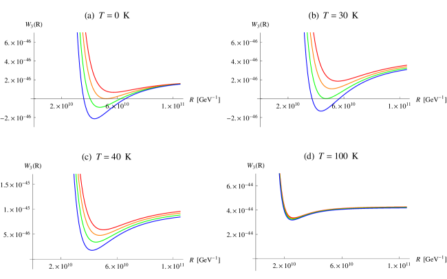
Figure 1: The RHS of equation (16), $W_{3}(R)$, as a function of the compactification radius $R$ for normal hierarchy Dirac neutrinos with the lightest neutrino mass of $6\times 10^{-12}{\rm\ GeV}$ (red), $7\times 10^{-12}{\rm\ GeV}$ (orange), $8\times 10^{-12}{\rm\ GeV}$ (green), and $9\times 10^{-12}{\rm\ GeV}$ (blue) for temperatures: (a) $T=0$, (b) $T=30\ \rm K$, (c) $T=40\ \rm K$, and (d) $T=100\ \rm K$, respectively. Note that the ranges in figures (c) and (d) are larger than for the first two plots. $M_{\rm pl}$ has been set to 1 for simplicity.

Here we discuss the finite temperature effects for the case of one dimension compactified on a circle. Working in four dimensions, we consider the spacetime interval,

$$ds^{2}=g_{(3)\mu\nu}\,dx^{\mu}dx^{\nu}+R(t)^{2}\,d\phi^{2}\ ,$$ (3)

where $g_{(3)\mu\nu}$ is the metric on the noncompact 3D spacetime with $\mu,\nu=0,1,2$, and the compact coordinate $\phi\in[0,2\pi)$. We assume a homogeneous and isotropic 3D metric,

$$g_{(3)\mu\nu}=\left(\begin{array}[]{ccc}-1&0&0\\ 0&\frac{a(t)^{2}}{1-\kappa\,r^{2}}&0\\ 0&0&a(t)^{2}\,r^{2}\\ \end{array}\right)\ ,$$ (7)

where $a(t)$ is the scale factor of the noncompact space, and $\kappa=1,0,\mbox{\rm or}-1$ corresponds to a closed, flat, or open metric, respectively. We choose a stress-energy tensor consistent with the symmetries of the metric,

$$T^{\mu}_{\ \ \nu}=\left(\begin{array}[]{cccc}-\rho_{3}&0&0&0\\ 0&p_{3}&0&0\\ 0&0&p_{3}&0\\ 0&0&0&p_{R}\\ \end{array}\right)\ ,$$ (12)

where $\rho_{3}$ is the energy density, and $p_{3},p_{R}$ are the pressures in the noncompact and compact space, respectively, all being functions of $R$ and $\beta=1/(k_{B}T)$, with $T$ – temperature. Einstein’s equations (2) take the form,

$$2\,\frac{\dot{a}}{a}\frac{\dot{R}}{R}+\frac{\dot{a}^{2}}{a^{2}}+\frac{\kappa}{a^{2}}=\frac{\rho_{3}}{M_{\rm pl}^{2}}\ ,$$ (13)

$$\frac{\ddot{R}}{R}+\frac{\dot{a}}{a}\frac{\dot{R}}{R}+\frac{\ddot{a}}{a}=-\frac{p_{3}}{M_{\rm pl}^{2}}\ ,$$ (14)

$$2\,\frac{\ddot{a}}{a}+\frac{\dot{a}^{2}}{a^{2}}+\frac{\kappa}{a^{2}}=-\frac{p_{R}}{M_{\rm pl}^{2}}\ .$$ (15)

Here the dot denotes the derivative with respect to time. This yields the equation of motion for $R$,

$$\frac{\ddot{R}}{R}+2\frac{\dot{a}}{a}\frac{\dot{R}}{R}=\frac{1}{M_{\rm pl}^{2}}\left(-p_{3}+\frac{1}{2}\,\rho_{3}+\frac{1}{2}\,p_{R}\right)\equiv W_{3}(R)\ .$$ (16)

The left hand side of (16) can be written as $-\square\log R$, where the d’Alembertian $\square\equiv D_{\mu}D^{\mu}$. The energy density and pressures are calculated from the free energy using standard thermodynamic relations Kolb ,

$$\rho_{3} = \frac{1}{2\pi R\,V_{2}}\frac{\partial\left(\beta F_{3}\right)}{\partial\beta}\bigg{|}_{a,R}\ ,$$ (17)

$$p_{3} = -\frac{1}{2\pi R}\frac{\partial F_{3}}{\partial V_{2}}\bigg{|}_{R,\beta}\ ,$$ (18)

$$p_{R} = -\frac{1}{2\pi V_{2}}\frac{\partial F_{3}}{\partial R}\bigg{|}_{a,\beta}\ ,$$ (19)

where $V_{2}$ is the volume of the noncompact space. The total free energy is obtained by summing the contributions from all standard model particles and the cosmological constant term. It is given by,

$$F_{3}=\sum_{\rm particles}F^{b/f}_{3}+2\pi R\,V_{2}\,\Lambda\ ,$$ (20)

where $\Lambda$ is the cosmological constant, and $F^{b/f}_{3}$ is the free energy for a particle of mass $m$. It is obtained by following the steps outlined in Kapusta ,

$$F^{b/f}_{3} \!=\! V_{2}\,(\pm\,d)\int\frac{d^{2}k}{(2\pi)^{2}}\sum_{n=-\infty}^{\infty}\bigg{[}\,\frac{1}{2}\sqrt{\vec{k}^{2}+m^{2}+\tfrac{n^{2}}{R^{2}}}$$ (21)

$$\ \ \ \ \ \ \ \ \ \ \ \ \ \ \ \ \ \ \ +\,\frac{1}{\beta}\log\left(1\mp e^{-\beta\sqrt{\vec{k}^{2}+m^{2}+\frac{n^{2}}{R^{2}}}}\right)\bigg{]}$$

$$\equiv V_{2}\left(\rho_{\rm Cas(3)}^{b/f}+f^{b/f}_{(3)}\right),$$

where the upper sign corresponds to bosons, the lower one to fermions, and $d$ is the number of degrees of freedom. The quantity $V_{2}\rho_{\rm Cas(3)}^{b/f}$ is the zero temperature Casimir energy and $V_{2}f^{b/f}_{(3)}$ is the finite temperature contribution to free energy.

It is straightforward to show that formula (20) is free of divergences. The 3D Casimir energy density for a particle of mass $m$ is given by,

$$\!\!\!\!\!\!\!\rho_{\rm Cas(3)}^{b/f}=\mp d\bigg{[}\frac{\Gamma\left(-2\right)}{16\pi}m^{4}R+\frac{m^{2}}{4\pi^{3}}\frac{1}{R}\sum_{n=1}^{\infty}\frac{1}{n^{2}}K_{2}(2\pi\,n\,m\,R)\bigg{]}$$ (22)

$$\ \ \ \ \ \ \ \ \equiv\rho_{\rm Cas(3)div}^{b/f}+\tilde{\rho}_{\rm Cas(3)}^{b/f}\ ,$$

where $K_{n}(x)$ is the modified Bessel function of the second kind, $V_{2}\rho_{\rm Cas(3)div}^{b/f}$ is the divergent part of the Casimir energy, and $V_{2}\tilde{\rho}_{\rm Cas(3)}^{b/f}$ is the finite regularized contribution. In the massless limit formula (22) reduces to,

$$\rho_{\rm Cas(3)}^{b/f}\Big{|}_{m=0}=\mp\,\frac{d}{720\,\pi R^{3}}\ .$$ (23)

Note here that,

$$\Lambda=\Lambda^{\rm obs}+\Lambda^{\rm q.corr.}\ ,$$ (24)

where the superscript “obs” indicates the observed value (i.e., $\Lambda^{\rm obs}\simeq 3.1\times 10^{-47}~{}{\rm GeV}^{4}$ pdg ), while “q.corr.” denotes the quantum correction in flat space given by,

$$\Lambda^{\rm q.corr.}=\sum_{\rm particles}(\pm\,d)\,\frac{\Gamma\left(-2\right)}{32\,\pi^{2}}m^{4}\ .$$ (25)

Since $\rho_{\rm Cas(3)div}^{b/f}=-2\pi R\,\Lambda^{\rm q.corr.}$, all the divergences cancel and the free energy can be expressed in terms of finite quantities using equation (20),

$$F_{3}/V_{2} = \sum_{\rm particles}\left[\tilde{\rho}^{b/f}_{\rm Cas(3)}+f^{b/f}_{(3)}\right]+2\pi R\,\Lambda^{\rm obs}$$ (26)

$$\equiv \tilde{\rho}_{{\rm Cas}\Lambda(3)}+f_{(3)}\ .$$

The first term in the second line of (26) is the Casmir energy including the cosmological constant term and has no temperature dependence. The second term is the finite temperature contribution.

In summary, the dynamics of the field $R$ is governed by equation (16), where $\rho_{3},p_{3},p_{R}$ are given by formulas (17)-(19), with the free energy expressed through equation (26). It is easy to check that equation (16) at zero temperature becomes the equation of motion resulting from the dimensionally reduced action, derived along the lines of Arkani , and takes the form,

$$\square\log R=\frac{R^{3}}{4\pi M^{2}_{\rm pl}}\left(\frac{\tilde{\rho}_{{\rm Cas}\Lambda(3)}}{R^{3}}\right)^{\prime}\ ,$$ (27)

where the prime indicates the derivative with respect to $R$.

It has been shown Arkani that depending on the neutrino masses, their type (Dirac or Majorana), and choice of hierarchy, there might exist a 3D anti de Sitter, Minkowski, or de Sitter vacuum of the low-energy effective theory. Including finite temperature effects has similar implications for all those cases, therefore, for illustrative purposes, we discuss only the case of Dirac neutrinos with normal hierarchy (figure 1). Note that the right hand side of equation (16), i.e., $W_{3}(R)$, is analogous to the derivative of the potential, so it should be equal to zero at the stationary points. In addition, $dW_{3}/dR<0$ at the stationary point implies stability, whereas $dW_{3}/dR>0$ corresponds to an unstable stationary point.

At temperatures $T\ll m_{e}\simeq 6\times 10^{9}\rm\ K$ only the photon, graviton, and neutrino contributions are relevant in equation (26). Figure 1 (a) shows the plot of $W_{3}(R)$ at $T=0$ for several lightest neutrino masses. In the cases for which stationary points exist, the one appearing at smaller $R$ is stable, whereas the one for larger $R$ is unstable. Those points match the ones found along the lines of Arkani . We checked that for low temperatures ($T\lesssim 10\rm\ K$) the finite temperature effects are negligible. However, as soon as the temperature reaches approximately 20 K, the curves slowly depart from the zero temperature result and move upwards. Figure 1 (b) shows the plot of $W_{3}(R)$ for $T=30\rm\ K$.

With temperature further increasing, each curve moves up and eventually fails to cross zero (figure 1 (c), (d)). At very high temperatures, the contributions from other standard model particles become relevant. We have investigated the behavior of $W_{3}(R)$ up to a temperature $T=100\ \rm GeV\simeq 10^{15}\rm\ K$ and confirmed that no zero points appear.

The behavior of $W_{3}(R)$ at high temperatures can be understood as follows. At a fixed temperature, only particles with Kaluza-Klein mass $m^{2}_{n}=m^{2}+n^{2}/R^{2}\lesssim T^{2}$ contribute to $f_{(3)}$, since the particles with larger masses are Boltzmann suppressed. In addition, particles with masses smaller than $T$ can be treated as radiation. Then, the finite temperature contributions to $W_{3}(R)$ coming from $\rho_{3}$ and $p_{3}$ (say $\rho^{T}_{3}$ and $p^{T}_{3}$, respectively) cancel because $p^{T}_{3}\simeq\rho^{T}_{3}/2$ at leading order. Equation (16) now becomes,

$$\!\!\!\!\!\!\!\!\!\!\!\!\!\!\!\frac{\ddot{R}}{R}+2\frac{\dot{a}}{a}\frac{\dot{R}}{R}$$

$$\!\!\!\!\!\!\!\!\!\!\simeq\frac{1}{2\pi R\,M_{\rm pl}^{2}}\left(\tfrac{3}{2}\tilde{\rho}_{{\rm Cas}\Lambda(3)}-\tfrac{1}{2}R\,\tilde{\rho}^{\prime}_{{\rm Cas}\Lambda(3)}-\tfrac{1}{2}R\,f^{T\prime}_{(3)}\right).$$ (28)

The first two terms on the right hand side are the zero temperature contributions. The third term is temperature dependent and can be estimated as $f^{T\,\prime}_{(3)}\sim-(TR)^{\prime}T^{3}=-T^{4}$, where the factor $(TR)$ comes from summing over Kaluza-Klein modes. Therefore, in the high temperature limit, equation (16) takes the form,

$$\square\log R=\frac{R^{3}}{4\pi M^{2}_{\rm pl}}\left(\frac{\tilde{\rho}_{{\rm Cas}\Lambda(3)}+\sigma_{3}R\,T^{4}}{R^{3}}\right)^{\prime},$$ (29)

where $\sigma_{3}$ encodes the number of standard model particles whose mass is smaller than $T$. For small $R$ we have $\tilde{\rho}_{{\rm Cas}\Lambda(3)}\sim 1/R^{3}$, so the first term on the right hand side of equation (29) is negligible for $T\gg 1/R$. Since for all experimentally allowed neutrino masses the zero temperature vacuum occurs at $R_{\rm vac}\approx 10^{10}{\ \rm GeV^{-1}}$, the high temperature limit applies for $T\gg 1000\ {\rm K}$. This confirms that finite temperature effects remove any zero points of $W_{3}(R)$ and, consequently, make the vacuum disappear. It also explains why the universe would have expanded rather than settle in a three-dimensional vacuum existing for small $R$ at zero temperature.

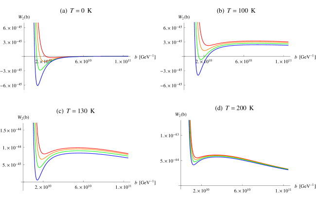
Figure 2: The RHS of equation (49), $W_{2}(b)$, as a function of the volume modulus $b$ for normal hierarchy Dirac neutrinos with the lightest neutrino mass of $1.0\times 10^{-11}{\rm\ GeV}$ (red), $1.5\times 10^{-11}{\rm\ GeV}$ (orange), $2.0\times 10^{-11}{\rm\ GeV}$ (green), and $2.5\times 10^{-11}{\rm\ GeV}$ (blue) for temperatures: (a) $T=0$, (b) $T=100\ \rm K$, (c) $T=130\ \rm K$, and (d) $T=200\ \rm K$, respectively. The ranges in figures (c) and (d) are larger than for the first two plots. $M_{\rm pl}$ has been set to 1 for simplicity.

II.2 Two-dimensional compactification

Next, we investigate the finite temperature structure of the standard model for a toroidal compactification. The four-dimensional spacetime interval is given by,

$$ds^{2}=g_{(2)\mu\nu}(x)\,dx^{\mu}dx^{\nu}+t_{ij}(x)\,dy^{i}dy^{j}\ .$$ (30)

The indices $\mu,\nu$ are now $0$ or $1$, and,

$$t_{ij}=\frac{b^{2}}{\tau_{2}}\left(\begin{array}[]{cc}1&\tau_{1}\\ \tau_{1}&|\tau|^{2}\\ \end{array}\right),$$ (33)

where $b^{2}$ and $\tau=\tau_{1}+i\tau_{2}$ are the volume and shape moduli, respectively. From here on we will assume $\tau=1/2+i\sqrt{3}/2$ in all formulas for the reasons discussed in AFW . We also assume a homogeneous universe, thus $b$ depends only on time. For the noncompact spacetime, we parametrize the line element as,

$$ds_{(2)}^{2}=-dt^{2}+a(t)^{2}dr^{2}.$$ (34)

The stress-energy tensor has the form,

$$T^{\mu}_{~{}~{}\nu}=\left(\begin{array}[]{cccc}-\rho_{2}&0&0&0\\ 0&p_{2}&0&0\\ 0&0&p_{b}&0\\ 0&0&0&p_{b}\end{array}\right),$$ (39)

where $\rho_{2}$, $p_{2}$, and $p_{b}$ are the energy density, pressure in the noncompact space, and pressure in the compact space, respectively.

We can now proceed along the same lines as in the previous section. The 4D free energy for a particle of mass $m$ is,

$$F^{b/f}_{2} \!=\! V_{1}\,(\pm\,d)\int\frac{dk}{2\pi}\sum_{n_{1},n_{2}=-\infty}^{\infty}\Bigg{[}\frac{1}{2}\sqrt{k^{2}+m^{2}+t^{ij}n_{i}n_{j}}$$ (40)

$$\ \ \ \ \ \ \ \ \ \ \ \ \ \ \ \ \ \ \ \ \ \ +\frac{1}{\beta}\log\left(1\mp e^{-\beta\sqrt{k^{2}+m^{2}+t^{ij}n_{i}n_{j}}}\right)\Bigg{]}$$

$$\equiv V_{1}\,\left(\tilde{\rho}^{b/f}_{{\rm Cas}(2)}+\rho^{b/f}_{{\rm Cas(2)div}}+f^{b/f}_{(2)}\right),$$

where $V_{1}$ is the volume of the 1D noncompact space and the terms in the last line are the finite part of the Casimir energy density, the divergent piece, and the temperature dependent contribution, respectively. As shown in AFW , the divergent part of the Casimir energy is cancelled by the quantum correction to the cosmological constant, just as in the previous case. The total free energy density in 2D is therefore given by,

$$F_{2}/V_{1} = \sum_{\rm particles}\left[\tilde{\rho}^{b/f}_{\rm Cas(2)}+f^{b/f}_{(2)}\right]+(2\pi b)^{2}\Lambda^{\rm obs}$$ (41)

$$\equiv \tilde{\rho}_{{\rm Cas}\Lambda(2)}+f_{(2)}\ ,$$

where the formula for $\tilde{\rho}^{b/f}_{\rm Cas(2)}$ is AFW ,

$$\!\!\!\!\!\!\!\!\!\tilde{\rho}^{b/f}_{\rm Cas(2)}=\tilde{\rho}^{b/f}_{\rm Cas(2)}(b,m)=\mp\,\frac{d}{(2\pi b)^{2}}$$

$$\!\!\!\!\!\!\!\times\Bigg{[}2\left(\tfrac{4}{3}\right)^{1/8}(b\,m)^{3/2}\sum_{p=1}^{\infty}\frac{1}{p^{3/2}}K_{3/2}\left(2\left(\tfrac{3}{4}\right)^{1/4}\pi\,p\,b\,m\right)$$

$$\ +\,\sqrt{3}\,(b\,m)^{2}\sum_{p=1}^{\infty}\frac{1}{p^{2}}K_{2}\left(2\left(\tfrac{4}{3}\right)^{1/4}\pi\,p\,b\,m\right)$$

$$\ +\,4\left(\tfrac{3}{4}\right)^{1/4}\sum_{n,p=1}^{\infty}\frac{1}{p^{3/2}}\left(n^{2}+\tfrac{2}{\sqrt{3}}\,(b\,m)^{2}\right)^{3/4}$$

$$\ \ \ \ \times(-1)^{pn}\,K_{3/2}\left(\pi\,p\,\sqrt{3\,n^{2}+2\sqrt{3}\,(b\,m)^{2}}\right)\!\Bigg{]}.$$ (42)

In the second line of equation (41), $\tilde{\rho}_{{\rm Cas(2)}\Lambda}$ is the contribution at zero temperature including the cosmological constant term, while $f_{(2)}$ is the temperature dependent piece. The energy density and pressure are calculated from the total free energy as before,

$$\rho_{2} =\left.\frac{1}{(2\pi b)^{2}V_{1}}\frac{\partial\left(\beta F_{2}\right)}{\partial\beta}\right|_{a,b}\ ,$$ (43)

$$p_{2} =-\frac{1}{(2\pi b)^{2}}\left.\frac{\partial F_{2}}{\partial V_{1}}\right|_{b,\beta}\ ,$$ (44)

$$p_{b} =-\frac{1}{8\pi^{2}V_{1}b}\left.\frac{\partial F_{2}}{\partial b}\right|_{a,\beta}\ .$$ (45)

Einstein’s equations take the form,

$$2\,\frac{\dot{a}\,\dot{b}}{a\,b}+\frac{\dot{b}^{2}}{b^{2}}=\frac{\rho_{2}}{M_{\rm pl}^{2}}\ ,$$ (46)

$$2\,\frac{\ddot{b}}{b}+\frac{\dot{b}^{2}}{b^{2}}=-\frac{p_{2}}{M_{\rm pl}^{2}}\ ,$$ (47)

$$\frac{\ddot{a}}{a}+\frac{\dot{a}\,\dot{b}}{a\,b}+\frac{\ddot{b}}{b}=-\frac{p_{b}}{M_{\rm pl}^{2}}\ ,$$ (48)

and yield,

$$\frac{\ddot{b}}{b}+\frac{\dot{a}\,\dot{b}}{a\,b}+\frac{\dot{b}^{2}}{b^{2}}=-\Box{\,\log{b}}=\frac{1}{2M_{\rm pl}^{2}}(\rho_{2}-p_{2})\equiv W_{2}(b)\ .$$ (49)

As in the previous case, the right hand side of (49), i.e., $W_{2}(b)$, governs the dynamics of the volume modulus of our compact space. Stationary points are given by zeros of $W_{2}(b)$. Similar arguments as before show that, in the cases for which stationary points exist, the one appearing at smaller $b$ is stable, and the one for larger $b$ is unstable. The $T=0$ results match the numbers obtained in AFW . We checked that those zero points also disappear with increasing temperature. As an example, figure 2 shows the behavior of $W_{2}(b)$ for Dirac neutrinos with normal hierarchy for different temperatures and masses.

At high temperature the relation $p^{T}_{2}\simeq\rho^{T}_{2}$ (where $\rho^{T}_{2}$ and $p^{T}_{2}$ are the temperature dependent parts of the energy density and pressure, respectively) is satisfied at leading order. One can show at next-to-leading order that $\rho^{T}_{2}-p^{T}_{2}\sim(b\,T)^{2}\,T\sim T^{3}$, where the factor $(b\,T)^{2}$ again comes from summing Kaluza-Klein modes. Consequently, equation (49) becomes,

$$-\Box{\,\log{b}}\simeq\frac{1}{M_{\rm pl}^{2}}\left(\frac{\tilde{\rho}^{b/f}_{{\rm Cas}\Lambda(2)}}{(2\pi b)^{2}}+\sigma_{2}\,b^{2}\,T^{3}\right),$$ (50)

where $\sigma_{2}$ is mass dimension three and contains information on the number of standard model particles whose mass is smaller than $T$. Thus $W_{2}(b)$ is an increasing function of temperature, and for high enough $T$ the zero points are washed out. As before, we conclude that there shouldn’t have been a “two-dimensional” epoch in the history of our universe yet.

III Transitions between spacetimes

The possibility of transitions between spacetimes of different dimensionality is certainly interesting to explore Sean ; Pillado ; Graham ; Salem ; Adamek . In our case, as noted in the previous section, there are no vacua at high temperature, thus no transition of this type could have occurred in the early universe. This is in accordance with observation. Obviously, the current visible universe is still four-dimensional, which also agrees with the dynamics of the compact dimensions presented in the previous section.

Nevertheless, it seems interesting to investigate the possibility of a future tunneling of our 4D de Sitter universe to a lower-dimensional anti de Sitter spacetime, which we have shown to exist for appropriate neutrino types and masses. Since the current temperature is $T\simeq 2.7\rm\ K$ and the universe is cooling down, we can safely calculate the transition rates using the zero temperature potential (as was shown in the previous section, for $T\lesssim 10\rm\ K$ finite temperature effects are negligible).

III.1 4D $\rightarrow$ 2D transitions

We first note that a transition of our 4D (false) vacuum to a 2D$\times T^{2}$ anti de Sitter (true) vacuum AFW is only possible if the geometry of two spatial dimensions of our 4D universe is that of a “very large” torus. The solutions interpolating between 4D and 2D$\times T^{2}$ regions are black holes with toroidal horizons and such transitions correspond to nucleation of those black holes in the 4D de Sitter spacetime. In calculating the transition rate we follow the usual method outlined in Sean . The prescription is simple: we take any finite Euclidean solution connecting one side of the potential barrier with the other, calculate the instanton action, and use this to estimate the transition rate.

The equations of motion are derived from relations (46)-(48) in the limit $T\rightarrow 0$. The two independent equations reduce to,

$$2\frac{\ddot{b}}{b}+\frac{\dot{b}^{2}}{b^{2}}=\frac{\tilde{\rho}_{{\rm Cas}\Lambda(2)}}{(2\pi b)^{2}M_{\rm pl}^{2}}\ ,$$ (51)

$$a=C\,\dot{b}\ ,$$ (52)

where $C$ is a constant determined by initial conditions. Analyzing numerically the dynamics of $b(t)$ we confirmed that the anti de Sitter vacuum found in AFW is indeed stable.

The transition rate is given by,

$$\Gamma=\Gamma_{0}\,e^{-(S_{\rm inst}[b]-S_{dS_{4}})}\ ,$$ (53)

where $\Gamma_{0}$ is a constant, the 4D de Sitter action is Sean ,

$$S_{dS_{4}}=-24\,\pi^{2}\frac{M_{\rm pl}^{4}}{\Lambda^{\rm obs}}\sim-10^{122}\ ,$$ (54)

and $S_{\rm inst}[b]$ is the instanton action. The equations of motion in Euclidean space are obtained by flipping the sign of the potential in equation (51), as a consequence of the analytic continuation $t\rightarrow i\tau$. $S_{\rm inst}[b]$ can be estimated using a finite numerical (interpolating) solution of the Euclidean equations of motion connecting both sides of the potential barrier (equivalently, connecting points on both sides of the Euclidean potential stable point). We numerically found finite solutions for the initial conditions $b(0)=b_{0}$ and $\dot{b}(0)=0$ for a range of $b_{0}$ values. Various finite solutions correspond to nucleating black holes of different mass in the 4D spacetime. One of such solutions, assuming normal hierarchy Dirac neutrinos with the lightest neutrino mass of $10^{-11}\ \rm GeV$, is shown in figure 3. Using this solution, the Coleman-de Luccia-like instanton action can be calculated as Sean ,

$$-S_{\rm inst}[b] = -8\pi^{3}M_{\rm pl}^{2}\int d\tau\left[\ddot{a}\,b^{2}-a\,\dot{b}^{2}+a\frac{\tilde{\rho}_{{\rm Cas}\Lambda(2)}}{(2\pi M_{\rm pl})^{2}}\right]$$ (55)

$$\simeq 10^{61}\ll-S_{dS_{4}}\ .$$

One can also estimate the transition rate by calculating the Hawking-Moss-like instanton action which describes $b(t)$ sitting at the unstable de Sitter vacuum (at $b=b_{dS}$) as,

$$-S_{\rm HM\,inst}=16\,\pi^{3}(M_{\rm pl}b_{dS})^{2}\simeq 10^{61}\ll-S_{dS_{4}}\ .$$ (56)

The Hawking-Moss-like instanton is of the same order as the Coleman-de Luccia-like instanton obtained via the interpolating solution. Such a result was expected since the interpolating solution should be equal to the solution at the top of the de Sitter hill in the limit $b_{0}\rightarrow b_{dS}$. In both cases the transition rate is,

$$\Gamma\sim e^{S_{dS_{4}}}\sim e^{-10^{122}}\ .$$ (57)

This is an extremely small number, so it is clear that these transitions are highly suppressed.

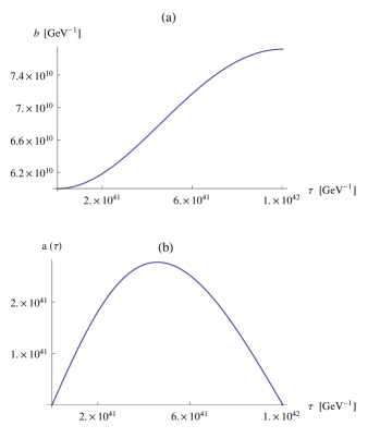
Figure 3: (a) The solution $b(\tau)$ of the Euclidean equivalent of equation (51) assuming normal hierarchy Dirac neutrinos with the lightest neutrino mass of $10^{-11}\ \rm GeV$ and for the initial conditions $b(0)=6\times 10^{10}{\rm\ GeV^{-1}}$ and $\dot{b}(0)=0$. (b) The corresponding solution $a(\tau)$ of the Euclidean version of equation (52).

III.2 4D $\rightarrow$ 3D transitions

We now examine the possibility of transitions from the 4D de Sitter (false) vacuum to a 3D$\times S^{1}$ anti de Sitter (true) vacuum Arkani . In the previous subsection we found that the instanton action corresponding to the transition to a lower-dimensional universe calculated via the Hawking-Moss-like instanton gives a result of the same order as the interpolating solution. Here we proceed the other way around and first estimate the transition rate to a 3D spacetime by calculating the Hawking-Moss-like instanton. Equations of motion at zero tempereture can be obtained from relations (13)-(15) by taking $T\rightarrow 0$ as in the previous 2D case.

Now, we have to rewrite and solve these equations in Euclidean space. We first note that there exists an analytic continuation to Euclidean space yielding a finite instanton solution only for an open metric ansatz ($\kappa=-1$) Sean . The equations of motion have the same form as equations (13)-(15) after the limit $T\rightarrow 0$ is taken, but with the substitution $\tilde{\rho}_{{\rm Cas}\Lambda(3)}\rightarrow-\tilde{\rho}_{{\rm Cas}\Lambda(3)}$. In order to calculate the instanton, we take the solution sitting at the unstable de Sitter vacuum, i.e., at the top of the $\tilde{\rho}_{{\rm Cas}\Lambda(3)}$ de Sitter hill (at $R=R_{0}$). The equations now yield,

$$\frac{\dot{a}^{2}}{a^{2}}-\frac{1}{a^{2}}+\frac{\tilde{\rho}_{{\rm Cas}\Lambda(3)}(R_{0})}{2\pi R_{0}M^{2}_{\rm pl}}=0\ ,$$ (58)

$$\ddot{a}+\frac{\tilde{\rho}_{{\rm Cas}\Lambda(3)}(R_{0})}{2\pi R_{0}M^{2}_{\rm pl}}a=0\ .$$ (59)

Since $\bar{V}_{(3)}(R_{0})>0$, these equations have a solution around the de Sitter vacuum given by,

$$a(\tau)=\frac{\sin(\omega_{0}\tau)}{\omega_{0}}$$ (60)

with $\omega_{0}^{2}=\tilde{\rho}_{{\rm Cas}\Lambda(3)}(R_{0})/(2\pi R_{0}M_{\rm pl}^{2})$. The Hawking-Moss-like instanton can now be approximated by Sean ,

$$S_{\rm HM\,inst}=-8\,\pi^{3}\left(\frac{2\pi M_{\rm pl}^{6}R_{0}^{3}}{\tilde{\rho}_{{\rm Cas}\Lambda(3)}({R_{0}})}\right)^{\frac{1}{2}}.$$ (61)

Using $R_{0}\simeq 10^{11}~{}{\rm GeV}^{-1}$ and $V_{(3)}(R_{0})\simeq 10^{-35}~{}{\rm GeV}^{3}$, we obtain $S_{\rm HMinst}\simeq-10^{92}$. The absolute value of this number is much larger than the 2D case result from the previous section, however, it is still orders of magnitude smaller than $-S_{dS_{4}}$. The transition rate is again extremely suppressed.

We will now search for finite interpolating solutions. Contrary to the 2D case, most of the solutions are singular and one has to adopt a different strategy. We look for finite solutions around the minimum of the Euclidean potential, as was presented in Sean . From equation (27), one obtains,

$$\ddot{R}+2\frac{\dot{a}}{a}\dot{R}=-\frac{1}{2\pi M_{\rm pl}^{2}}\left(\tfrac{3}{2}\tilde{\rho}_{{\rm Cas}\Lambda(3)}-\tfrac{1}{2}R\,\tilde{\rho}^{\prime}_{{\rm Cas}\Lambda(3)}\right)\ .$$ (62)

After plugging $R=R_{0}+\delta R$ and using relation (60), equation (62) becomes,

$$\!\!\!\!\ddot{\delta R} +2\omega_{0}\cot(\omega_{0}\tau)\,\dot{\delta R}$$

$$\!\!\!\!\!\!\!\!+\!\frac{1}{2\pi M_{\rm pl}^{2}}\left[\tilde{\rho}_{{\rm Cas}\Lambda(3)}^{\prime}(R_{0})\!-\!\tfrac{1}{2}R_{0}\tilde{\rho}_{{\rm Cas}\Lambda(3)}^{\prime\prime}(R_{0})\right]\!\delta R=0\ .$$ (63)

This equation has a solution expressed in terms of Gegenbauer polynomials $C^{(\alpha)}_{n}$ Sean ,

$$\delta R=KC^{(1)}_{n}\left(\cos(\omega_{0}\tau)\right)\ ,$$ (64)

where $K\ll R_{0}$ is a constant, and the index $n$ satisfies the relation,

$$n^{2}\!+\!2n\!-\!\frac{1}{2\pi M^{2}_{\rm pl}\omega^{2}_{0}}\!\left[\tilde{\rho}_{{\rm Cas}\Lambda(3)}^{\prime}(R_{0})\!-\!\tfrac{1}{2}R_{0}\tilde{\rho}_{{\rm Cas}\Lambda(3)}^{\prime\prime}(R_{0})\right]=0\,.$$

In order to have non-singular solutions, the Gegenbauer index $n$ must be a non-negative integer. We find that this condition can only be satisfied for normal hierarchy Dirac neutrinos with the lightest neutrino mass $\simeq 7.4\times 10^{-12}{\rm\ GeV}$. A quick check shows that this mass is associated with a stable 3D de Sitter vacuum, so the tunneling process is forbidden.

However, as mentioned in Sean , it might be possible to obtain non-singular solutions in another way, i.e., by carefully fine-tuning the initial conditions rather than looking for a solution around the unstable de Sitter vacuum. Nevertheless, even if a non-singular solution exists, it is expected to yield an instanton action of the same order as the Hawking-Moss-like instanton action. Consequently, the transition rate is extremely small.

IV Conclusions

In this paper, we have investigated the structure of the standard model coupled to gravity at finite temperature for one- and two-dimensional compactifications (on a circle and on a torus). For each case, we have calculated the energy density and pressures from the free energy. Those quantities enter Einstein’s equations, which govern the evolution of the compactified spacetime at finite temperature. We have found that stationary points of the equation of motion for the size of the compact space disappear with increasing temperature. The precise temperature at which this happens depends on the neutrino masses, their hierarchy, and whether the neutrinos are Dirac or Majorana, but the qualitative behavior is the same.

For the compactification on a circle we have shown numerically, as an example, that the stable stationary point disappears at temperatures on the order of tens of Kelvin, for the lightest neutrino mass of $\sim 10^{-11}\mbox{\rm~{}GeV}$, choosing the neutrinos to be Dirac with normal hierarchy. With increasing temperature, the stationary point never reappears. We have shown analytically that such behavior is expected in the high temperature limit. The case of the 2D compactification on a torus is very similar.

Finally, we have calculated the transition rates for tunneling between vacua of different dimensionality at zero temperature. Following the steps outlined in Sean , we found Coleman-de Luccia-like instanton solutions for a tunneling from a 4D de Sitter universe to a spacetime with two spatial dimensions compactified on a torus. The rate for such a process turned out to be extremely suppressed. For the case of tunneling to a spacetime with one spatial dimension compactified on a circle, we found only the Hawking-Moss-like instanton solution, which also yields a negligible transition rate.

Nevertheless, under the condition that the universe has the right topology, because the transition rates at low temperatures are not zero, a tunneling process to a lower-dimensional spacetime might be the ultimate fate of our universe.

Acknowledgment

The authors would like to express their special thanks to Mark Wise for inspirational discussions and many extremely helpful comments at all stages of the work on this paper. We further thank Sean Carroll, Matthew Johnson and Yu Nakayama for very useful remarks. The work was supported in part by the U.S. Department of Energy under contract No. DE-FG02-92ER40701. K.I. acknowledges the support of the Gordon and Betty Moore Foundation.

References

- (1) N. Arkani-Hamed, S. Dubovsky, A. Nicolis and G. Villadoro, Quantum horizons of the standard model landscape, JHEP 0706, 078 (2007) [arXiv:hep-th/0703067].
- (2) J. M. Arnold, B. Fornal, M. B. Wise, Standard model vacua for two-dimensional compactifications, JHEP 1012, 083 (2010) [arXiv:1010.4302 [hep-th]].
- (3) S. M. Carroll, M. C. Johnson and L. Randall, Dynamical compactification from de Sitter space, JHEP 0911, 094 (2009) [arXiv:0904.3115 [hep-th]].
- (4) F. S. Accetta and E. W. Kolb, Finite-temperature instability for compactification, Phys. Rev. D 34, 1798 (1986).
- (5) J. I. Kapusta and C. Gale, Finite-temperature field theory, Cambridge University Press, Cambridge U.K. (2006).
- (6) K. Nakamura et al. [Particle Data Group], Review of particle physics, J. Phys. G 37, 075021 (2010).
- (7) J. J. Blanco-Pillado, D. Schwartz-Perlov and A. Vilenkin, Transdimensional tunneling in the multiverse, JCAP 1005, 005 (2010) [arXiv:0912.4082 [hep-th]].
- (8) P. W. Graham, R. Harnik and S. Rajendran, Observing the dimensionality of our parent vacuum, Phys. Rev. D 82, 063524 (2010) [arXiv:1003.0236 [hep-th]].
- (9) J. J. Blanco-Pillado and M. P. Salem, Observable effects of anisotropic bubble nucleation, JCAP 1007, 007 (2010) [arXiv:1003.0663 [hep-th]].
- (10) J. Adamek, D. Campo and J. C. Niemeyer, Anisotropic Kantowski-Sachs universe from gravitational tunneling and its observational signatures, Phys. Rev. D 82, 086006 (2010) [arXiv:1003.3204 [hep-th]].