Entanglement of polar molecules in pendular states

Abstract

In proposals for quantum computers using arrays of trapped ultracold polar molecules as qubits, a strong external field with appreciable gradient is imposed in order to prevent quenching of the dipole moments by rotation and to distinguish among the qubit sites. That field induces the molecular dipoles to undergo pendular oscillations, which markedly affect the qubit states and the dipole-dipole interaction. We evaluate entanglement of the pendular qubit states for two linear dipoles, characterized by pairwise concurrence, as a function of the molecular dipole moment and rotational constant, strengths of the external field and the dipole-dipole coupling, and ambient temperature. We also evaluate a key frequency shift, $\triangle\omega$, produced by the dipole-dipole interaction. Under conditions envisioned for the proposed quantum computers, both the concurrence and $\triangle\omega$ become very small for the ground eigenstate. In principle, such weak entanglement can be sufficient for operation of logic gates, provided the resolution is high enough to detect the $\triangle\omega$ shift unambiguously. In practice, however, for many candidate polar molecules it appears a challenging task to attain adequate resolution. Simple approximate formulas fitted to our numerical results are provided from which the concurrence and $\triangle\omega$ shift can be obtained in terms of unitless reduced variables.

I Introduction

Since the original proposal by DeMille Demille , arrays of ultracold ($<$ 1 mK) polar molecules have come to be considered among the most promising platforms to implement a quantum computer  carr ; Book2009 ; Friedrich ; Lee ; Kotochigova ; yelin ; Micheli ; Charron ; kuz ; ni ; lics ; YelinDeMille . His proposal describes a complete scheme for quantum computing using as qubits the dipole moments of diatomic molecules, trapped in a one-dimensional optical lattice, partially oriented in an external electric field, and coupled by the dipole-dipole interaction. The qubit states are individually addressable because the field has an appreciable gradient so the Stark effect is different for each location in the array.

A subsequent proposal has advocated coupling polar molecules into a quantum circuit using superconducting wires wallraff . Such capacitive, electrodynamic coupling to transmission line resonators is analogous to coupling to Rydberg atoms and Cooper pair boxes sorensen ; andre . The molecular qubits are entangled via the coupling to the transmission lines rather than direct dipole-dipole interactions. Again, addressability of the qubits is achieved via the Stark effect by means of local gating of an electrostatic field.

Entanglement is a major ingredient in most quantum computation algorithms. It is among the defining features of quantum mechanics, with no classical analog Book ; Book2 ; Siegfried . A pure state of a pair of quantum systems is said to be entangled if its wavefunction cannot be factored into a product of wavefunctions of the individual partners. For example, the singlet state of two spin-$\frac{1}{2}$ particles, $\frac{1}{\sqrt{2}}(|\uparrow\downarrow\rangle-|\downarrow\uparrow\rangle)$ is entangled. A mixed state is entangled if it cannot be represented as a mixture of factorizable pure states. The allure of quantum information processing has recently motivated studies of entanglement for a variety of potential qubit systemsentg-kais ; Vedral ; Osterloh ; Amico ; Su ; Dur ; Cincio ; Charron ; Lee ; Kotochigova ; Osenda1 ; Osenda2 ; Osenda3 ; Osenda4 ; Xu ; Wei . These include one-dimensional arrays of localized spins, coupled through exchange interactions and subject to an external magnetic field entg-kais and analogous treatments of trapped electric dipoles coupled by dipole-dipole interactions Wei .

However, the previous studies of entanglement of electric dipoles have not adequately considered how the external electric field, integral to current designs for quantum computers using polar molecules, affects both the qubit states and the dipole-dipole interaction. For the simplest case of a ${}^{1}\Sigma$ diatomic molecule, the qubit eigenstates resulting from the Stark effect are linear combinations of spherical harmonics, with coefficients that depend markedly on the field strength. These are appropriately termed pendular states  Friedrich2 , or field-dressed states Ticknor . In such states, the orientation of the dipole moment has a broad angular range (not solely along or opposed to the field direction as are spins in a magnetic field). Likewise, the dipole-dipole interaction for molecules in pendular states is much different than that for dipoles in the absence of an external field.

Here we evaluate entanglement, as measured by pairwise concurrence, for the prototype case of two diatomic polar molecules in pendular states, ultracold and trapped in distinct optical lattice sites. The molecules are represented as identical rigid dipoles, undergoing angular oscillations, a fixed distance apart and subject either to a different or to the same external electric field. We examine the dependence of the concurrence on three dimensionless variables. The first governs the energy and intrinsic angular shape of the qubits (when the dipole-dipole interaction is switched off). It is $\mu$$\mathbf{\varepsilonup}$/$B$, the ratio of the Stark energy (magnitude of permanent dipole moment times electric field strength) to the rotational constant (proportional to inverse of molecular moment of inertia). The second variable governs the magnitude of the dipole-dipole coupling. It is $\Omega/B$, with $\Omega$ = ($\mu^{2}/r^{3}$), the square of the permanent dipole moment divided by the cube of the separation distance. The third variable, $k_{B}T/B$, is the ratio of thermal energy (Boltzmann constant times Kelvin temperature) to the rotational constant.

We also examine an aspect related to but distinct from entanglement. The operation of a quantum gate Jones such as CNOT requires that manipulation of one qubit (target) depends on the state of another qubit (control). This is characterized by the shift, $\triangle\omega$, in the frequency for transition between the target qubit states when the control qubit state is changed. The shift $\triangle\omega$, which is due to the dipole-dipole interaction, must be kept smaller than the differences required to distinguish among addresses of qubit sites. Under conditions envisaged in the proposed designs Demille ; carr ; Book2009 ; Friedrich ; Lee ; YelinDeMille for quantum computing with trapped polar molecules, $\Omega/B<10^{-4}$, and for the ground eigenstate both the entanglement and frequency shift $\triangle\omega$ become very small. For CNOT and other operations, entanglement needs to be large, but can be induced dynamically, so need not be appreciable in the ground eigenstate. Yet a small $\triangle\omega$ shift can only suffice if the resolution is high enough to detect the shift unambiguously. From estimates of the line widths of transitions between the pendular qubit states, we find it an open question whether adequate resolution can be obtained for typical candidate diatomic molecules.

II ENTANGLEMENT FOR TWO DIPOLES IN PENDULAR STATES

II.1 Hamiltonian terms and pendular qubit states

The Hamiltonian for a single trapped linear polar molecule in an external electric field is

$${\bf H}=\frac{p^{2}}{2m}+V_{trap}({\bf r})+B\bf{J}^{2}-\bm{\mu}\cdot\text{\Large\bm{$\varepsilonup$}}$$ (1)

where the molecule, with mass $m$, rotational constant $B$ and body-fixed dipole moment $\mu$, has translational kinetic energy $p^{2}/2m$, potential energy $V_{trap}$ within the trapping field, and rotational energy $B\bf{J}^{2}$ as well as interaction energy $\bm{\mu}\cdot$$\varepsilonup$ with the external field $\varepsilonup$. In the trapping well, at ultracold temperatures, the translational motion of the molecule is quite modest and very nearly harmonic; $p^{2}/2m+V_{trap}({\bf r})$ thus is nearly constant and can be omitted from the Hamiltonian. There remains the rotational kinetic energy and Stark interaction,

$${\bf H_{S}}=B\bf{J}^{2}-{\bf\mu}\text{\Large$\mathbf{\varepsilonup}$}\text{cos}\theta$$ (2)

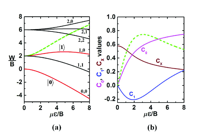
Figure 1: (Color online) Stark states for a polar diatomic molecule in a ${}^{1}\Sigma$ electronic state Hughes , as functions of $\mu$$\mathbf{\varepsilonup}$$/B$, with $\bf\mu$ the permanent dipole moment, $\varepsilonup$ the field strength, $B$ the rotational constant. (a) Eigenenergies, W, and (b) Matrix elements of orientation cosines; see Eq.(14). States used as qubits (red curves) are labeled $|0\rangle$ and $|1\rangle$. In the field-free limit, $|0\rangle$ correlates with the $J=0$, $M_{J}=0$ and $|1\rangle$ with the $J=1$, $M_{J}=0$ rotational states. Dashed curve (green) in (a) shows energy for transition between qubit states, $\triangle W=W_{1}-W_{0}$; that in (b) shows $C_{0}-C_{1}$, difference between effective dipole moments, projections of the molecular dipole on the field direction for pendular states $|0\rangle$ and $|1\rangle$.

which represent a spherical pendulum with $\theta$ the polar angle between the molecular axis and the field direction. Figure 1(a) displays the lowest few pendular eigenenergies Hughes for a ${}^{1}\Sigma$ diatomic (or linear) molecule, as functions of $\mu$$\varepsilonup$/$B$. These are labeled with the familiar quantum numbers $\tilde{J}$, M that specify the field-free rotational states. However, $\tilde{J}$ wears a tilde to indicate it is no longer a good quantum number since the Stark interaction mixes the rotational states, whereas M (denoting the projection of the ${\mathbf{J}}$-vector on the field direction) remains good as long as azimuthal symmetry about $\varepsilonup$ is maintained. As proposed by DeMille, the qubit states $|0\rangle$ and $|1\rangle$ are chosen as the lowest M = 0 pendular states, with $\tilde{J}$ = 0 and 1, respectively. These are superpositions of $Y_{j,0}$ spherical harmonics,

$$|0\rangle=\sum_{j}a_{j}Y_{j,0}(\theta,\varphi),\;\;\;\;\;\;\;\;\;\;|1\rangle=\sum_{j}b_{j}Y_{j,0}(\theta,\varphi)$$ (3)

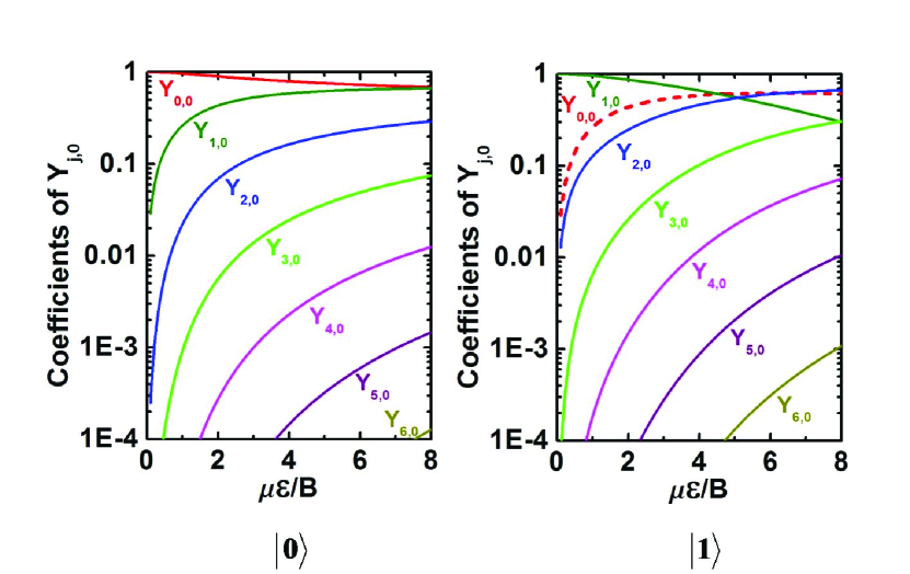
Figure 2: (Color online) Coefficients of sums of spherical harmonics for pendular states $|0\rangle$ and $|1\rangle$, see Eq.(3). Dashed curve for $|1\rangle$ indicates the coefficient of $Y_{0,0}$ is negative.

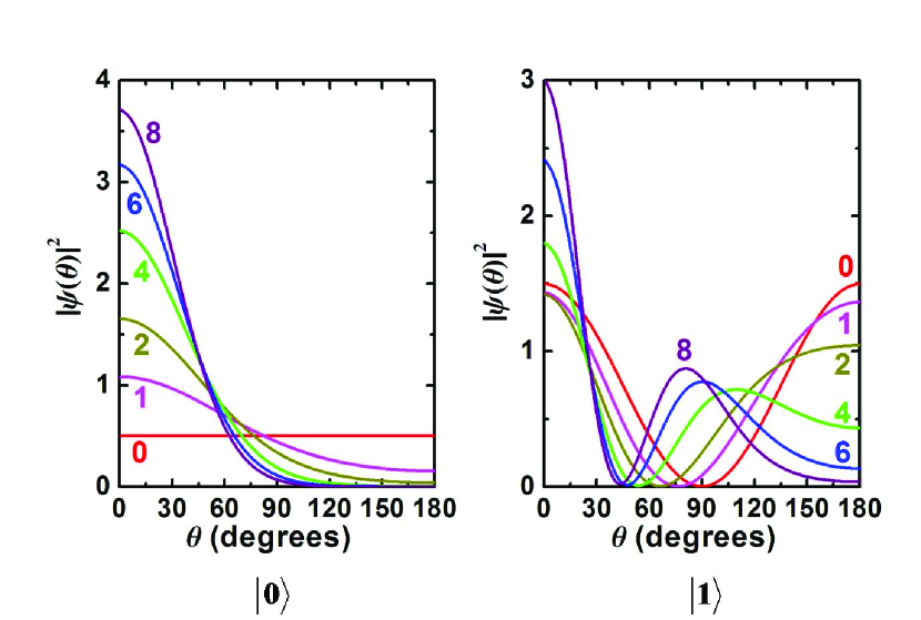
Figure 3: (Color online) Angular distributions of the $|0\rangle$ and $|1\rangle$ pendular states for values of $\mu$$\varepsilonup$$/B$ between 0 and 8.

Figure 2 plots the coefficients as functions of $\mu$$\varepsilonup$/$B$. Figure 3 displays the angular distributions of the pendular qubit states. For $|0\rangle$ the distribution is unimodal and as $\mu$$\varepsilonup$/$B$ increases the dipole orientation increasingly favors the direction of the $\varepsilonup$-field (at $\theta$ = $0^{o}$). For $|1\rangle$ the distribution is bimodal because, with M = 0, the dipole is rotating perpendicular to the ${\mathbf{J}}$-vector, which is perpendicular to the field direction. For $\varepsilonup$ = 0, the dipole orientation is equally probable in the hemispheres toward ($\theta<90^{o}$) or opposite ($\theta>90^{o}$) to the field direction. As $\mu$$\varepsilonup$/$B$ increases, the pinwheeling dipole favors the opposite hemisphere because there its motion is slowed because the Stark interaction becomes unfavorable. However, when $\mu$$\varepsilonup$/$B$ becomes large enough, pinwheeling is inhibited and converted into pendular libration about the field direction, so the dipole orientation shifts to favor the toward hemisphere.

Adding a second trapped polar molecule, identical to the first but distance $r_{12}$ apart, introduces in addition to its pendular term the dipole-dipole coupling interaction,

$$V_{d-d}=\frac{\bm{\mu}_{1}\cdot\bm{\mu}_{2}-3(\bm{\mu}_{1}\cdot{\bf n})(\bm{\mu}_{2}\cdot{\bf n})}{|{\bf r}_{1}-{\bf r}_{2}|^{3}}$$ (4)

Here n denotes a unit vector along ${\bf r}_{12}$. In the presence of an external field, it becomes appropriate to express $V_{d-d}$ in terms of angles related to the field direction. As shown in Appendix A, the result after averaging over azimuthal angles (that for M = 0 states are uniformly distributed) reduces to

$$V_{d-d}=\Omega(1-3\text{cos}^{2}\alpha)\text{cos}\theta_{1}\text{cos}\theta_{2}$$ (5)

where $\Omega=\mu^{2}/r_{12}^{3}$, the angle $\alpha$ is between the ${\bf r}_{12}$ vector and the field direction and polar angles $\theta_{1}$ and $\theta_{2}$ are between the ${\bm{\mu}}_{1}$ and ${\bm{\mu}}_{2}$ dipoles and the field direction. Until later (Sec. IV), we consider the external field magnitude and direction to be the same at the sites of both the polar molecules.

II.2 Entanglement measured by pairwise concurrence

We will deal with the entanglement of formation, $\mathfrak{E}(\rho)$, which characterizes the amount of entanglement needed in order to prepare a state described by a density matrix, $\rho$. (Henceforth, we term $\mathfrak{E}(\rho)$ just ”entanglement”, for short.) Wootters Wootters ; Hill has shown that $\mathfrak{E}(\rho)$ for a general state of two qubits can be quantified by the pairwise $\it concurrence$, $C(\rho)$, which ranges between zero and unity. The relation can be written as

$$\mathfrak{E}(\rho)=\xi(C(\rho))$$ (6)

where $\xi$ is given by

$$\xi(C)=h\left(\frac{1+\sqrt{1-C^{2}}}{2}\right)$$ (7)

with $h(x)=-x\text{log}_{2}x-(1-x)\text{log}_{2}(1-x)$. The function $\xi(C)$ increases monotonically between zero and unity as $C$ varies from 0 to unity. The concurrence is given by

$$C(\rho)=max\left\{0,\sqrt{\lambda_{1}}-\sqrt{\lambda_{2}}-\sqrt{\lambda_{3}}-\sqrt{\lambda_{4}}\right\}$$ (8)

where the $\lambda_{i}$’s are the eigenvalues, in decreasing order, of the non-Hermitian matrix $\rho\tilde{\rho}$, where $\tilde{\rho}$ is the density matrix of the spin-flipped state, defined as

$$\tilde{\rho}=(\sigma_{y}\otimes\sigma_{y})\rho^{*}(\sigma_{y}\otimes\sigma_{y})$$ (9)

with $\rho^{*}$ the complex conjugate of $\rho$ and $\sigma_{y}$ a Pauli matrix. The parent density matrix $\rho$ is taken in the basis formed by combining the pendular qubit states; for a pair of two-level particles, this comprises the four state vectors $\{|00\rangle,|01\rangle,|10\rangle,|11\rangle\}$.

In order to evaluate thermal entanglement, we need a temperature dependent density matrix, $\rho=\text{exp}(-\beta H)/Z(T)$, with $\beta=1/k_{B}T$ and $Z(T)$ the partition function

$$Z(T)=tr[\text{exp}(-\beta H)]=\sum_{i}g_{i}e^{-\beta E_{i}}$$ (10)

with $E_{i}$ the $i^{th}$ eigenvalue and $g_{i}$ its degeneracy. Hence the density matrix can be written as

$$\rho(T)=\frac{1}{Z}\sum_{i}^{N}e^{-\beta E_{i}}|\Psi_{i}\rangle\langle\Psi_{i}|$$ (11)

where $|\Psi_{i}\rangle$ is the $i^{th}$ eigenfunction. From the density matrix $\rho(T)$, we can obtain the reduced density matrix for any pair of dipoles and thence evaluate the concurrence at any temperature.

III Concurrence of two dipoles in pendular states

We illustrate the calculation of pairwise concurrence for $N=2$ dipoles. The Hamiltonian, $H_{S1}$ + $H_{S2}$ + $V_{d-d}$, when set up in a basis of the qubit pendular states, $\{|00\rangle,|01\rangle,|10\rangle,|11\rangle\}$, takes the form,

$${\bf H_{S1}+H_{S2}}=\left(\begin{array}[]{cccc}W_{0}+W_{0}^{\prime}&0&0&0\\ 0&W_{0}+W_{1}^{\prime}&0&0\\ 0&0&W_{1}+W_{0}^{\prime}&0\\ 0&0&0&W_{1}+W_{1}^{\prime}\end{array}\right)$$ (12)

$${\bf V_{d-d}}=\Omega(1-3\text{cos}^{2}\alpha)\left(\begin{array}[]{cccc}C_{0}C_{0}^{\prime}&C_{0}C_{X}^{\prime}&C_{X}C_{0}^{\prime}&C_{X}C_{X}^{\prime}\\ C_{0}C_{X}^{\prime}&C_{0}C_{1}^{\prime}&C_{X}C_{X}^{\prime}&C_{X}C_{1}^{\prime}\\ C_{X}C_{0}^{\prime}&C_{X}C_{X}^{\prime}&C_{1}C_{0}^{\prime}&C_{1}C_{X}^{\prime}\\ C_{X}C_{X}^{\prime}&C_{X}C_{1}^{\prime}&C_{1}C_{X}^{\prime}&C_{1}C_{1}^{\prime}\end{array}\right)$$ (13)

where $W_{0}$ and $W_{1}$ are the eigenenergies of the pendular qubit states $|0\rangle$, and $|1\rangle$, in the absence of the dipole-dipole interaction. Primes attached to quantities for the second dipole indicate that the external field magnitude may differ at its site (although, as noted above, we postpone evaluating that case until Sec. IV). In $V_{d-d}$ the basis qubit states are linked by matrix elements containing factors arising from the orientation cosines in Eq. (5); these are

$$C_{0}=\langle 0|\text{cos}\theta|0\rangle;\;\;\;\;C_{X}=\langle 0|\text{cos}\theta|1\rangle;\;\;\;\;C_{1}=\langle 1|\text{cos}\theta|1\rangle$$ (14)

$C_{0}$ and $C_{1}$ are the expectation values of cos$\theta$ in the pendular states $|0\rangle$ and $|1\rangle$, respectively, so represent for those states the effective dipole moment projections displayed in Fig.1(b). $C_{X}$ corresponds to an exchange interaction or transition dipole moment between the qubit states. Both the Stark eigenenergies $W_{i}$ and the dipole-dipole elements $C_{k}$ are functions of $\mu$$\varepsilonup$/$B$. As seen in Fig.1(b), as $\mu$$\varepsilonup$/$B$ is increased $C_{0}$ becomes increasingly positive, whereas $C_{1}$ is increasingly negative until about $\mu$$\varepsilonup$/$B$ = 2, then climbs to zero at about $\mu$$\varepsilonup$/$B$ = 4.9 and thereafter is increasingly positive. The range $\mu$$\varepsilonup$/$B$ = 2 to 4 is recommended for the proposed quantum computer designs Demille ; andre ; within that range, the difference in the effective dipole moments of the qubits, $|C_{0}-C_{1}|$, varies only modestly.

If the dipole-dipole interaction is omitted ($\Omega$ = 0), the eigenvectors of $H_{S1}$ + $H_{S2}$ are simply $\Psi_{1}=|00\rangle$, $\Psi_{2}=2^{-1/2}(|10\rangle-|01\rangle)$, $\Psi_{3}=2^{-1/2}(|10\rangle+|01\rangle)$, $\Psi_{4}=|11\rangle$, corresponding to the eigenenergies of Eq.(12). For $\Psi_{1}$ and $\Psi_{4}$, which are obviously nonentangled states, the concurrence is zero. For $\Psi_{2}$ and $\Psi_{3}$, which exemplify fully entangled states, the concurrence is unity; these are termed Bell states Book .

When the dipole-dipole coupling is included, an analytical solution to obtain eigenstates is only feasible when the external field is switched off. As shown in Appendix B, in that limit analytical results can be obtained for each step in evaluating the concurrence, both for the four individual eigenstates and their combination in the thermal concurrence. As seen in Fig. 1, for $\mu$$\varepsilonup$/$B$ = 0, the energy terms in Eq.(12) involve merely $W_{0}$ = 0 and $W_{1}$ = 2$B$. In the $V_{d-d}$ matrix of Eq.(13), the cosine matrix elements $C_{0}$ and $C_{1}$ vanish and $C_{X}$ = $3^{-1/2}$; thus, the only nonzero elements occur along the antidiagonal and (for $\alpha$ = $90^{o}$) are just $\Omega C_{X}^{2}$. The results for this zero-field limit prove useful in interpreting those for the general pendular case.

The limits with $\Omega$ = 0 and/or $\mu$$\varepsilonup$/$B$ = 0 motivate setting up the Hamiltonian of Eqs.(12) and (13), for the (unprimed) case with the same external field at both dipole sites, using a basis of Bell states:

$$\frac{|11\rangle+|00\rangle}{\sqrt{2}},\;\;\;\frac{|11\rangle-|00\rangle}{\sqrt{2}},\;\;\;\frac{|10\rangle+|01\rangle}{\sqrt{2}},\;\;\;\frac{|10\rangle-|01\rangle}{\sqrt{2}},$$ (15)

In this basis, the Hamiltonian becomes

$${\bf H_{S1}+H_{S2}}=\left(\begin{array}[]{cccc}W_{+}&W_{-}&0&0\\ W_{-}&W_{+}&0&0\\ 0&0&W_{+}&0\\ 0&0&0&W_{+}\end{array}\right)$$ (16)

$${\bf V_{d-d}}=\Omega(1-3\text{cos}^{2}\alpha)\left(\begin{array}[]{cccc}\hat{A}_{+}&\hat{B}&\hat{C}_{+}&0\\ \hat{B}&\hat{A}_{-}&\hat{C}_{-}&0\\ \hat{C}_{+}&\hat{C}_{-}&\hat{D}_{+}&0\\ 0&0&0&\hat{D}_{-}\end{array}\right)$$ (17)

Where $W_{\pm}=W_{1}\pm W_{0}$ and $\hat{A}_{\pm}=\frac{1}{2}(C_{1}^{2}+C_{0}^{2})\pm C_{X}^{2}$, $\hat{B}=\frac{1}{2}(C_{1}^{2}-C_{0}^{2})$, $\hat{C}_{\pm}=C_{X}(C_{1}\pm C_{0})$, $\hat{D}_{\pm}=C_{1}C_{0}\pm C_{X}^{2}$. This makes explicit a consequence of the symmetry between the (unprimed) sites Thankreviewer . In the Bell basis, the Hamiltonian factors, with the state $2^{-1/2}(|10\rangle-|01\rangle)$ in a $1\times 1$ block, so that state remains maximally entangled regardless of the value of $\mu$$\varepsilonup$/$B$ or $\Omega/B$.

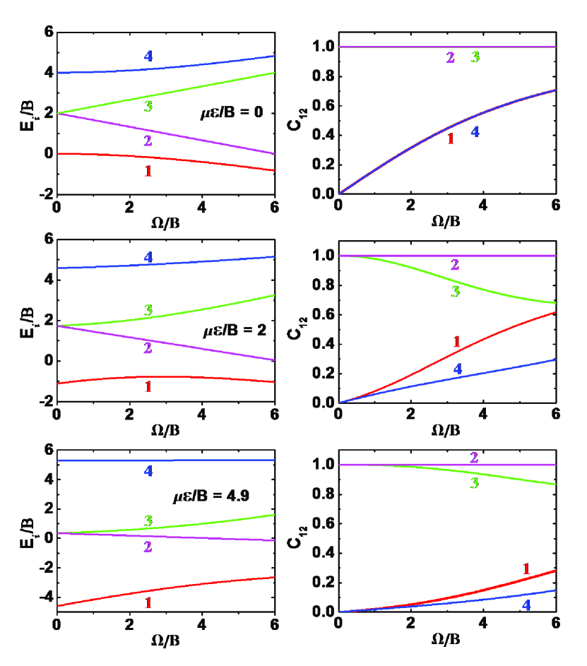
Figure 4: (Color online) Eigenenergies, numbered 1, 2, 3, 4 in order of increasing energy, and pairwise concurrences of the eigenstates for two dipoles as a function of the dipole-dipole coupling constant $\Omega/B$ for three values of the reduced electric field strength, $\mu$$\varepsilonup$$/B$ = 0, 2 and 4.9.

Figure 4 plots, for $\mu$$\varepsilonup$/$B$ = 0, 2 and 4.9, the eigenenergy and pairwise concurrence versus $\Omega/B$ = 0 to 6 for the four eigenstates of the two-dipole system. The eigenstates are numbered from 1 to 4 in order of increasing energy. For $\mu$$\varepsilonup$/$B$ = 0, both eigenstates 2 and 3 are Bell states, with eigenenergies $E_{i}/B$ = $2-(\Omega/6B)$ and $2+(\Omega/6B)$, respectively; eigenstates 1 and 4 are also entangled (much more weakly) by the dipole-dipole interaction, with eigenenenergies that shift downwards and upwards nonlinearly with increasing $\Omega/B$, respectively. For $\mu$$\varepsilonup$/$B$ $>$ 0, the concurrences increase with $\Omega/B$ for eigenstates 1 and 4, and decrease for eigenstate 3. By virtue of the symmetry imposed factorization noted above, eigenstate 2 retains the same Bell form despite the Stark and dipole-dipole interactions which affect its energy, and its concurrence is always unity. For small $\Omega/B<<1$, eigenstate 3 also becomes independent of the dipole-dipole interaction and coincides with eigenstate 2 in both energy and concurrence. For $\mu$$\varepsilonup$/$B$ = 4.9, as seen in Fig. l(b), the $C_{1}=\langle 1|\text{cos}\theta|1\rangle$ factor that appears in seven of the matrix elements in Eq. (13) vanishes. Consequently, the energy of eigenstate 4 then becomes independent of the dipole-dipole interaction, although its wavefunction and concurrence do not.

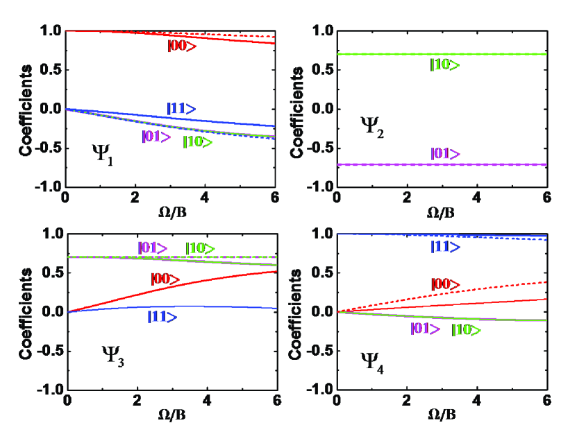
Figure 5: (Color online) Eigenvectors of the four eigenstates for two dipoles as a function of the dipole-dipole coupling constant $\Omega/B$ = 0 to 6 for $\mu$$\varepsilonup$$/B$ = 0 (dashed curves) and 2 (solid curves).

Figure 5 shows, for $\mu$$\varepsilonup$/$B$ = 0 and 2, how the contributions of the basis states to each of the eigenstates vary with the strength of the dipole-dipole interaction. This illustrates that for $\Omega/B<<1$ the eigenstates rapidly approach those for $\Omega$ = 0. Indeed, we find that for $\Omega/B<0.04$ the concurrences for eigenstates 1 and 4, which rapidly become the same, are proportional to $\Omega/B$ within better than 1%. Thus,

$$C_{12}=K(x)[\Omega/B]$$ (18)

where the proportionality factor $K(x)$ is a function of $x$ = $\mu$$\varepsilonup$/$B$. At the zero-field limit, $K(0)=1/6$. In Appendix C we describe a numerical analysis that provided an accurate approximate formula,

$$K(x)=A_{1}+\frac{A_{2}}{1+\text{exp}[(x-x_{0})/\triangle x]}$$ (19)

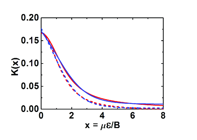
Figure 6: (Color online) The $K(x)$ function of Eq.(18); solid curves show exact result (red) and fitted function (blue) of Eq.(19) that pertains to pendular qubit basis, see Eq.(3). For comparison, dashed curve pertains to field-free basis with $|0\rangle$ = $Y_{0,0}$, $|1\rangle$ = $Y_{1,0}$ (Cf. Table III, Appendix C).

This is plotted in Fig.6 and values of the four parameters are listed in Appendix C.

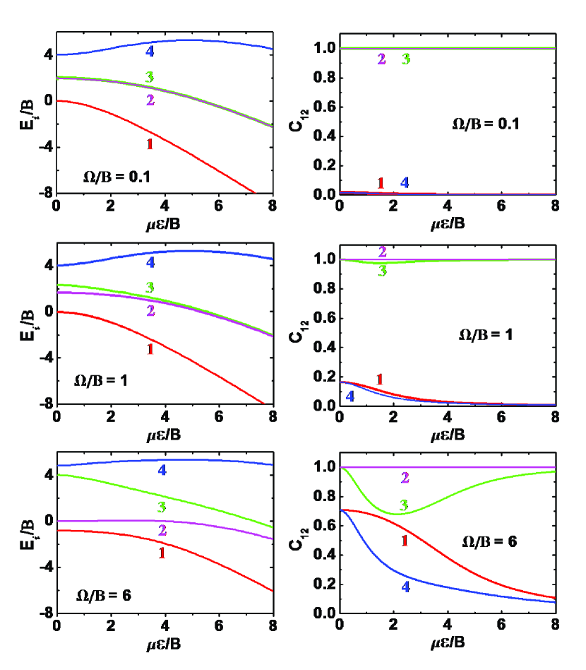
Figure 7: (Color online) Eigenenergies and concurrences for the four eigenstates for two dipoles as a function of reduced variables, $\mu$$\varepsilonup$$/B$ for electric field and $\Omega/B$ for dipole-dipole coupling.

Figure 7 displays for $\Omega/B$ = 0.1, 1 and 6 the eigenenergies and concurrences versus $\mu$$\varepsilonup$/$B$ from 0 to 8 for the four eigenstates. As the dipole-dipole interaction increases 60-fold over this range, its effect on the eigenstate energies is relatively modest, whereas the concurrences change markedly, in response to variations in eigenvector compositions such as illustrated in Fig. 5.

Figure 8 gives a contour plot of the thermal pairwise concurrence derived from Eq.(11) as a function of $\Omega/B$ and $k_{B}T/B$. It pertains to $\mu$$\varepsilonup$/$B$ = 3; we found that normalizing the thermal concurrence to its value for T = 0 and $\Omega/B$ = 1 removed most of the variation with $\mu$$\varepsilonup$/$B$ from such contour plots. For T = 0, the thermal concurrence coincides with that for the ground state, eigenstate $\Psi_{1}$. However, as $k_{B}T/B$ increases, the thermal concurrence decreases and is always smaller than the ground-state concurrence. This may seem odd, because Eq.(11) specifies a shift in population that reduces the contribution from the gound state, while bringing in contributions from the excited states. The eigenstates 2 and 3 then populated have large concurrence, so increasing temperature might be expected to make the net thermal concurrence become larger than for the ground-state, rather than smaller. The source of this behavior is indicated by the analytic solution obtained in Appendix B for the zero-field limit,

$$C_{12}(\text{T})=C_{12}(1)P_{1}-C_{12}(2)P_{2}-C_{12}(3)P_{3}-C_{12}(4)P_{4}$$ (20)

where $P_{i}=(1/Z)\text{exp}(-E_{i}/k_{B}T)$ with $Z(T)=\sum_{i}\text{exp}(-E_{i}/k_{B}T)$. This shows that the excited states indeed reduce the thermal concurrence, an effect traceable to Eq.(8) and which persists even for large $\mu$$\varepsilonup$/$B$.

Another striking aspect of Fig. 8 is that the concurrence vanishes along and outside a particular contour. That contour defines mutually dependent maximum values of $k_{B}T/B$ and minimum values of $\Omega/B$ required to obtain nonzero concurrence. When $\Omega/B<<1$, we find that a modified form of Eq.(18) represents the thermal concurrence,

$$C_{12}(\text{T})=\text{max}\{0,K(x)[y-y_{0}(x,z)]\}$$ (21)

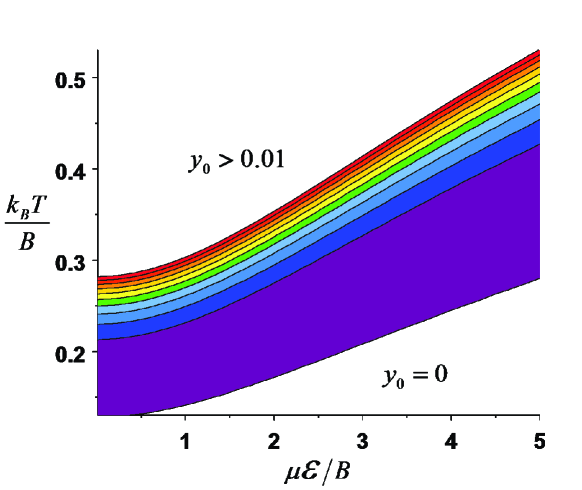
Figure 9: (Color online) Contour plot displaying $y_{0}(x,z)$ term in Eq.(21) vs. $x$ = $\mu$$\varepsilonup$$/B$. Within each colored band, the range of $y_{0}$ is 0.001; thus in the lowest colored band (magenta). $y_{0}$ ranges between 0 and 0.001; in the highest colored band (red), $y_{0}$ is between 0.009 and 0.01.

Here $x$ = $\mu$$\varepsilonup$/$B$; $y$ = $\Omega/B$; and $z=k_{B}T/B$ is the scaled temperature. Fig. 9 gives a contour plot of $y_{0}=\Omega_{c}/B$, the critical dipole-dipole coupling required for nonzero concurrence. Some further details are included in Appendix B.

The original proposal by DeMille and kindred papers on quantum computing with trapped polar molecules Demille ; carr ; Lee ; yelin ; kuz ; YelinDeMille ; andre discuss for several examples the range of experimental conditions deemed suitable and acceptable. For trap temperatures of the order of a microkelvin or below, the typical values of $k_{B}T/B$ are a few times $10^{-6}$, so indicate that only ground-state entanglement would be significant. The external field strengths considered are typically a few $kV/cm$. The spacing between optical lattice sites, $r=\lambda/2$, is half the optical lattice wavelength. The optimal choice of $\lambda$ ranges between 1 to 0.3 microns, depending on electronic transition frequencies of the molecules to be trapped YelinDeMille . From these parameters and molecular data, values of $\Omega/B$ are small; we find for a dozen potential candidate molecules values ranging between $4\times 10^{-6}$ (for KCs) to $2\times 10^{-4}$ (for CsI). A favorite candidate is SrO ($\mu=8.9D$, $B=0.33$ $cm^{-1}$, $\lambda=1$ micron), for which $\Omega/B\sim 10^{-5}$. In that regime, the concurrence is simply proportional to $\Omega/B$, so can be easily evaluated from Eq.(18) and/or (21) without use of the rather elaborate prescription outlined in Eqs.(6-14).

IV Frequency shift for two coupled dipoles in pendular states

In the region $\Omega/B<10^{-4}$, the concurrence of the ground eigenstate is very small, typically $<10^{-5}$. However, such meager entanglement in eigenstates can still be adequate for quantum computing, as demonstrated with NMR versions of quantum computers Jones2 . The key aspect is that although entanglement needs to be large for some quantum computing algorithms, it need not be appreciable or even present in the ground eigenstate of the system; it can be induced dynamically during operation of the computer Zhou . Here, for the polar molecule case, we consider this aspect. We also evaluate an eigenstate property, a small frequency shift, distinct from but related to the pairwise concurrence, that is important for quantum computing.

The need for selective excitation in operation of quantum logic gates Jones ; Seth ; Cory is an essential feature. Taking the 2-qubit CNOT gate as an example, its operation requires that manipulation of one qubit (target) is perceptively affected by the state of the other qubit (control). In our case, the qubits are pendular states that can be accessed by microwave transitions, which offer high spectral resolution. As resolution has a crucial role, we now suppose the external field differs enough at the two dipole sites (denoted unprimed and primed) to supply distinct addresses for the sites (cf. Fig. 1(a), green dashed curve).

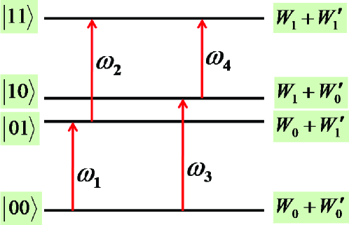
Figure 10: (Color online) Schematic energy levels for qubit pendular eigenstates of N = 2 dipoles, in absence of dipole-dipole interaction, thus corresponding to Eq.(12). Qubit basis states shown at left, eigenenergies at right. Pairs of transitions involved in CNOT operation are indicated: $\omega_{1}$ transfers dipole 2 from $|0\rangle$ to $|1\rangle$ with dipole 1 remaining in $|0\rangle$; then $\omega_{2}$ transfers dipole 1 from $|0\rangle$ to $|1\rangle$ with dipole 2 remaining in $|1\rangle$. Analogously, the same result could be reached by $\omega_{3}$ followed by $\omega_{4}$. Transition energies (including dipole-dipole terms to first-order) are given in Eqs.(23).

Since $\Omega/B$ is so small, we first omit the dipole-dipole interaction and, as illustrated in Fig. 10, consider transitions among the pendular eigenstates of Eq.(12). Although in this limit the ground-state concurrence is zero, as seen in Eq.(18), it is possible to generate states of large concurrence by use of resonant pulses Zhou ; Thanks . Start by applying a pulse resonant with the transition denoted $\omega_{1}$, between $|00\rangle$ and $|01\rangle$, which has energy $W^{\prime}_{1}-W^{\prime}_{0}$. Note that $\omega_{1}$ needs to be well-resolved from the transition $\omega_{3}$, between $|00\rangle$ and $|10\rangle$, which has energy $W_{1}-W_{0}$. The separation thus comes from the different values of the external field at the two sites (plus a dipole-dipole contribution, in higher order). The requisite field strength difference, $\varepsilonup$^′ - $\varepsilonup$, can be readily determined from another approximation formula,

$$(W_{1}-W_{0})/B=A_{1}+\frac{A_{2}}{1+\left(x/x_{0}\right)^{p}}$$ (22)

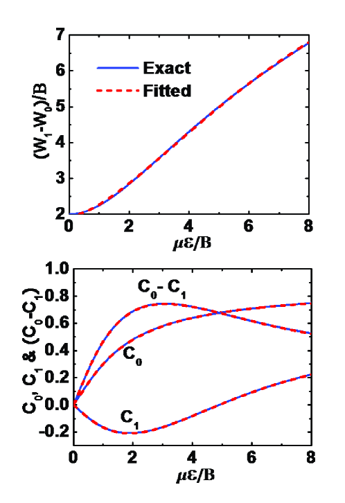
Figure 11: (Color online) Comparison of exact results (blue curves) with fitted approximation functions (dashed red curves) for properties governing transitions among qubit states, Eqs.(23): pendular energy difference, $(W_{1}-W_{0})/B$, cosine expectation values, $C_{0}$ and $C_{1}$ and their difference, $C_{0}-C_{1}$; cf. Eqs. (22, 25, 26).

by comparing results for $x$ = $\mu$$\varepsilonup$/$B$ and $x^{\prime}$ = $\mu^{\prime}$$\varepsilonup$^′/$B$; the accurate fit obtained (better than 1% except near $x=0$) is displayed in Fig. 11 and the four parameters in Eq.(22) are given in Appendix C. The amplitude and duration of the $\omega_{1}$ pulse can be adjusted to make it a $\pi/2$ pulse, which will put the system in the state $2^{-1/2}(|00\rangle+|01\rangle)$.

Next, to complete the CNOT gate, apply a pulse resonant with the transition $\omega_{2}$ between $|01\rangle$ and $|11\rangle$. This needs to be well-resolved from transition $\omega_{3}$ between $|00\rangle$ and $|10\rangle$. However, in our initial approximation, both $\omega_{2}$ and $\omega_{3}$ have the same transition energy, $W_{1}-W_{0}$. Hence, weak as it is, the dipole-dipole interaction is seen to have an essential role: to introduce a frequency shift, $\triangle\omega=\omega_{3}-\omega_{2}$, adequate for unambiguous resolution. If that is fulfilled, the amplitude and duration of the $\omega_{2}$ pulse can be adjusted to make it a $\pi$ pulse. Thereby the system will be put in the state $2^{-1/2}(|00\rangle+|11\rangle)$. This result of a CNOT gate is to first approximation a Bell state (aside from small corrections of order $\Omega/B$), so its concurrence will be near unity. It is not an eigenstate, so will evolve with time but in principle would remain nearly fully entangled until degraded by other interactions.

If now the dipole-dipole terms from Eq.(13) are included to first order, we obtain

$$\omega_{1}=\langle 01|\hat{H}|01\rangle-\langle 00|\hat{H}|00\rangle=W^{\prime}_{1}-W^{\prime}_{0}+\Omega_{\alpha}C_{0}(C^{\prime}_{1}-C^{\prime}_{0})$$ (23a)

$$\omega_{2}=\langle 11|\hat{H}|11\rangle-\langle 01|\hat{H}|01\rangle=W_{1}-W_{0}+\Omega_{\alpha}C^{\prime}_{1}(C_{1}-C_{0})$$ (23b)

$$\omega_{3}=\langle 10|\hat{H}|10\rangle-\langle 00|\hat{H}|00\rangle=W_{1}-W_{0}+\Omega_{\alpha}C^{\prime}_{0}(C_{1}-C_{0})$$ (23c)

$$\omega_{4}=\langle 11|\hat{H}|11\rangle-\langle 10|\hat{H}|10\rangle=W^{\prime}_{1}-W^{\prime}_{0}+\Omega_{\alpha}C_{1}(C^{\prime}_{1}-C^{\prime}_{0})$$ (23d)

where $\Omega_{\alpha}=\Omega(1-3\text{cos}^{2}\alpha)$. Thus, the key frequency shift is given by

$$\triangle\omega=\omega_{3}-\omega_{2}=\omega_{4}-\omega_{1}=\Omega_{\alpha}(C_{1}-C_{0})(C^{\prime}_{1}-C^{\prime}_{0})$$ (24)

For given $\Omega_{\alpha}$, the frequency shift $\triangle\omega$ depends only on $x$ and $x^{\prime}$, which determine at the respective sites the difference in the effective dipole moment projections $C_{0}$ and $C_{1}$ along the external electric field, specified in Eq.(14). To provide a convenient means to evaluate Eqs.(23) and (24) we again fitted our numerical results to obtain accurate approximation formulas,

$$C_{0}(x)=A_{1}+\frac{A_{2}}{1+\left(x/x_{0}\right)^{p}}$$ (25)

$$C_{1}(x)=A_{0}+\frac{A_{1}}{1+\text{exp}[(x-x_{1})/\triangle x_{1}]}+\frac{A_{2}}{1+\text{exp}[-(x-x_{2})/\triangle x_{2}]}$$ (26)

These functions are plotted in Fig. 11, together with $C_{0}-C_{1}$, and the fitted parameters are given in Appendix C.

Since for small $\Omega/B$, both the concurrence and $\triangle\omega$ are proportional to $\Omega/B$, the frequency shift provides an equivalent measure of entanglement. When the $\varepsilonup$-fields differ at the two sites, Eq.(18) still provides a very accurate approximation for $C_{12}(x,x^{\prime})$, merely by replacing the proportionality factor by the geometric mean, $[K(x)K(x^{\prime})]^{1/2}$. The concurrence (which involves $C_{X}$, the exchange interaction term) is in principle different from $\triangle\omega$ but both have about the same magnitude. The frequency shift is much more relevant for quantum computing, because $\triangle\omega$ is directly involved in the CNOT gate.

Also important, in addition to the pulse shapes which affect the population transfers, are the durations of the resonant pulses required to resolve $\omega_{1}$ and $\omega_{2}$ from $\omega_{3}$; these must satisfy $\tau_{31}>>1/|\omega_{3}-\omega_{1}|$ and $\tau_{32}>>1/|\omega_{3}-\omega_{2}|$. For $\tau_{31}$ the lower bound usually can be made very low, permitting a short pulse duration. This holds because $\triangle$$\varepsilonup$ as well as dipole-dipole terms contribute to $|\omega_{3}-\omega_{1}|$, which thus can be made large by choice of the $\varepsilonup$-field gradient, regardless of whether $\Omega_{\alpha}$ is extremely small. In contrast, for $\tau_{32}$ the separation $\triangle\omega=|\omega_{3}-\omega_{2}|$ depends only on the dipole-dipole interaction. The smaller $\triangle\omega$ is, the longer the $\omega_{2}$ pulse duration has to be in order to complete the CNOT operation. Although larger $\triangle\omega$ allows a shorter pulse duration, $\triangle\omega$ must not be so large that it becomes comparable to or larger than the addressing shift produced by $\triangle$$\varepsilonup$, thereby thwarting correct identification of the qubits.

Table 1: Illustrative CNOT Gate Implementation^a.

$\mu$$\varepsilonup$/$B$	$x=1$	$x^{\prime}=1.01$	$x^{\prime}=1.10$		$x=3$	$x^{\prime}=3.03$	$x^{\prime}=3.30$
$(W_{1}-W_{0})/B$	2.2709	2.2759	2.3218		3.5614	3.5831	3.7789
$C_{0}$	0.30165	0.30404	0.32487		0.57922	0.58149	0.60051
$C_{1}$	-0.16467	-0.16573	-0.17461		-0.16362	-0.16150	-0.14115
$C_{0}-C_{1}$	0.46632	0.46977	0.49948		0.74284	0.74298	0.74165
$(\omega_{1}-\omega_{3})/B$		4.99E-3	5.09E-2			2.17E-2	2.17E-1
$\triangle\omega/B$		2.19E-6	2.33E-6			5.52E-6	5.51E-6
$C_{12}$		1.20E-6	1.17E-6			3.57E-7	3.34E-7

Table I provides specific numbers pertaining to the SrO example. From Sec.III, we take $\Omega_{\alpha}/B=10^{-5}$. As representative $\varepsilonup$-field values, we use $x$ = 1 and 3 for site 1 and and take $x^{\prime}$ higher by 1% or 10% for site 2. From Eqs.(23), the transition frequencies $\omega_{1}=\omega_{4}$ and $\omega_{2}=\omega_{3}$ (in units of $B$) to 5 or 6 significant figures. The frequency difference that must be resolvable for the first step of the CNOT operation, $\omega_{1}-\omega_{3}$, is approximately just $\triangle\triangle W=(W^{\prime}_{1}-W^{\prime}_{0})-(W_{1}-W_{0})$. From Fig. 11, this is seen to grow about linearly with both $x$ and $x^{\prime}-x$. The values in Table I (third row from bottom) range from $>10^{-3}$ to $>10^{-1}$ (in units of $B$). To accommodate more dipole qubits, it may be desired to make much smaller the $\varepsilonup$-field differences between sites; steps with $\triangle x$ = 0.01% were proposed by DeMille Demille . That might encounter engineering limitations, but in principle the proportionally smaller $\omega_{1}-\omega_{3}$ difference could still be readily resolved. For the second step of the CONT operation the crucial frequency shift, $\triangle\omega=\omega_{1}-\omega_{3}$ varies only modestly with $x$ and practically not at all with $x^{\prime}-x$. The values of $\triangle\omega/B$ in Table I (second row from bottom) range between 2 and $6\times 10^{-6}$; in frequency units, this range is 20 to 60 kHz. Smaller still are the corresponding values of the concurrence (bottom row); also insensitive to $x^{\prime}-x$ but, in accord with Fig. 6, varying more rapidly with $x$.

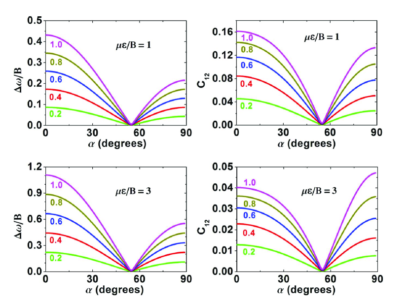
Figure 12: (Color online) Frequency shift $\triangle\omega/B$ (left panels) and ground state concurrence $C_{12}$ (right panels) as functions of $\alpha$, the orientation angle of the electric field. Curves are shown for $\Omega/B$ = 0.2 to 1.0 with $\mu$$\varepsilonup$/$B$ = 1 or 3.

Figure 12 exhibits for both the $\triangle\omega$ shift and concurrence the variation with $\alpha$, the angle between the direction of the electric field and the axis between the dipoles. This dependence enters via the factor ($1-3\text{cos}^{2}\alpha$) in the dipole-dipole interaction, Eq.(5), which emerges directly in the $\triangle\omega$ shift, Eq.(24), and by a more complex route propagates into the concurrence, via Eq.(13). Tilting the field direction to make $\alpha=54.73^{\circ}$, the ”magic angle”, provides a simple means to shut off the entanglement. That is a useful option, awkward to attain in other ways yelin ; YelinDeMille .

V Conclusions and prospects

In this study, our chief aim has been to examine entanglement of polar molecules by the dipole-dipole interaction and subject to an external electric field, for the prototype case of two diatomic or linear ${}^{1}\sum$ molecules. This required use of qubits that are pendular states comprised of sums of spherical harmonics. We focused on the pairwise concurrence and its dependence on three unitless reduced variables, involving the dipole moments, field strength, rotational constant, dipole-dipole coupling and temperature. We have considered a wide range of the parameters, to map general features of the concurrence. However, for conditions envisioned for proposed quantum computers, the dipole-dipole coupling is weak ($\Omega/B$ typically of order $10^{-4}$ to $10^{-6}$) and the concurrence becomes very small ($<10^{-5}$). For that weak coupling realm, we found the $\triangle\omega$ frequency shift provides an equivalent measure of entanglement, directly related to observable properties and hence preferable to the concurrence. We also obtained for both the $\triangle\omega$ shift and concurrence in the weak realm simple explicit formulas in terms of the reduced variables.

For quantum computing a crucial issue is whether $\triangle\omega$ is large enough to enable the $\omega_{2}$ transition to be reliably distinguished from $\omega_{3}$ (and, equivalently, $\omega_{1}$ from $\omega_{4}$). For typical candidate polar molecules, this requires resolving transitions separated by only tens of kHz. That would not be feasible in conventional molecular spectroscopy. Under ordinary gas phase conditions, transitions between molecular rotational or pendular states have line widths of the order of a few 100 kHz Townes . For ultracold molecules trapped in an optical lattice, line widths may be much narrower. Collisional broadening is eliminated and at microkelvin temperatures Doppler broadening is also quenched (as trap conditions are in the Lamb-Dicke regime). It is encouraging that for ultracold atoms extremely narrow line widths have been attained by exploiting ”magic” optical trapping conditions that are expected to be at least in part applicable to molecules Kotochigova2 . At present, however, no data have been reported on line widths for rotational transitions of ultracold molecules trapped in an optical lattice and subject to an external electric field. In view of the small size of $\triangle\omega$, it is important to obtain such data to assess the resolution attainable, since motion within the traps, coupling to lattice fields, and inhomogeneity of the external field may introduce appreciable line broadening.

We have sought to glean pertinent evidence from electric resonance spectroscopy of molecular beams, as the beams are collision free and transitions are observed in an external electric field (”Rabi C-field”). For BaO, both $\triangle M=0$, $J=0\rightarrow 1$ transitions in the microwave region xx and $\triangle J=0$, $|M|=0\rightarrow 1$ transitions in the radiofrequency region Wharton have been observed, in fields ranging from $\sim 200-500$ V/cm. For the radiofrequency transitions, line widths were only about 2 kHz, consistent with just the dwell time in the C-field. But for the microwave transitions the widths are much larger, 45 kHz; this is attributed both to the higher frequency of the transitions and to experimental conditions that render more significant Doppler broadening and nonuniformity of the field, especially in the entrance and exit fringe regions xw . The Doppler and dwell time contributions are not relevant to inferring what might be expected for trapped BaO (or SrO). Broadening by inhomogeneity of the external field is relevant but depends very much on experimental particulars. The transitions of interest, depicted in Fig. 10, occur in the microwave region and involve Stark fields typically ten-fold larger than used in the electric resonance spectroscopy, so the line widths might be significantly broadened due to field inhomogeneity. These observations do not permit firm conclusions about the resolution issue, but it decidedly poses an experimental challenge.

This discussion pertains only to the choice of qubits we have considered, pendular states of linear polar molecules, which involve transitions that change $\tilde{J}$ but not $M$. The resolution issue motivates examining other choices for qubits. For instance, states with the same $\tilde{J}$ but different $M$ could be used. Other options, particularly use of hyperfine or nuclear spin states instead of pendular states, have been suggested as means to reduce sources of decoherence Demille ; carr ; YelinDeMille ; andre . As yet, the size of $\triangle\omega$ for any qubit choice other than that used in this paper remains to be determined.

We intend to extend the treatment developed here to other choices for qubit basis states as well as to larger numbers $N>2$ of dipoles. In preliminary work on linear and planar arrays of dipoles up to $N=8$, we find, as expected, the maximum pairwise concurrence occurs for next-neighbor dipoles, although that for non-nearest ones is significant. Also in prospect is an analogous treatment of the proposed coupling of polar molecules via microwave strip-lines andre . There the entangling interaction differs from direct dipole-dipole interactions, but again the proposed qubits are pendular states.

Another pendular variant inviting attention is use of polar symmetric top molecules. The $|0\rangle$ and $|1\rangle$ qubits can be selected as $|J,K,M\rangle=|1,1,-1\rangle$ and $|1,1,+1\rangle$, which are degenerate in the field-free limit and thus have a first-order Stark effect Townes . Even in a weak electric field, these states are strongly oriented along and opposed to the field, with equal and opposite projections. Moreover, the effective dipole moments do not depend on the field strength so low fields can be used if necessary to reduce line broadening, without the penalty imposed by quenching of effective dipoles that would occur for the second-order Stark effect. At first blush, the symmetric top option appears to be disallowed because transitions between the $M$ = -1 and +1 Stark states violate the selection rules, $\triangle M=0$ or $\triangle M=\pm 1$. But the prohibition is not absolute. Because the optical lattice perturbs cylindrical symmetry about the field, $M$ is not strictly a ”good” quantum number, so the $\triangle M$ selection rule is relaxed. Moreover, if the molecule contains an atom with nuclear spin $I>1/2$, and hence an electric quadrupole moment, transitions with $\triangle M=\pm 2$ become allowed. For instance, a deuterium nucleius ($I=1$) makes $\triangle M=\pm 2$ transitions facile in Stark spectra Wofsy . Other symmetric top options for qubits are inversion doublets (e.g. in NH₃) or internal rotation states associated with hindered torsional motion (e.g. CH₃CF₃); these offer strong dipole-allowed transitions.

Previous studies of entanglement, both for polar molecules yelin ; Wei and for magnetic spins entg-kais ; Osenda1 ; Osenda2 ; Osenda3 ; Osenda4 ; Xu , have considered primarily domains where the concurrence is large ($>0.1$), and have focused on means to tune the entanglement to attain such domains. For polar molecules, that requires $\Omega/B>1$. Recently, it was suggested that such large $\Omega/B$ could be attained for dipole arrays by exploiting nanotraps with lattice spacing of the order of only 10 nm Wei . However, as emphasized in Sec. IV, for quantum computing large entanglement in the ground eigenstate is not required. Indeed, reducing the array spacing so markedly would strongly foster inelastic, spontaneous Raman scattering of lattice photons and hence induce decoherence Demille ; carr ; YelinDeMille . Such considerations make small rather than large $\Omega/B$, and consequently weak rather than strong entanglement in the ground eigenstate, actually preferable for quantum computing Wootters , provided resolution of the $\triangle\omega$ shift can be attained.

APPENDIX A: DIPOLE-DIPOLE INTERACTION

The angular dependence of the dipole-dipole interaction, given in Eq.(4), is usually expressed as

$$\Phi_{ij}=\text{cos}\beta-3\text{cos}\gamma_{i}\text{cos}\gamma_{j}$$ (A1)

where $\beta$ is the angle between dipoles $\mu_{i}$ and $\mu_{j}$; angles $\gamma_{i}$ and $\gamma_{j}$ specify the orientation of the dipoles with respect to the vector $r_{ij}$ between them. Ordinarily, it is natural (and done in all textbooks) to express $\text{cos}\beta$ in terms of the angles $\gamma$ together with the azimuthal angles $\phi_{r}$ about the $r_{ij}$ axis. Thus, use

$$\text{cos}\beta=\text{cos}\gamma_{i}\text{cos}\gamma_{j}+\text{sin}\gamma_{i}\text{sin}\gamma_{j}\text{cos}(\phi_{ri}-\phi_{rj})$$ (A2)

which when combined with the -3$\text{cos}\gamma_{i}\text{cos}\gamma_{j}$ term gives the familiar expression Stone . In the presence of the external electric field, we need to recast $\Phi_{ij}$ in terms of angles $\theta_{i}$ and $\theta_{j}$ that specify the orientation of the dipoles with respect to the direction of the external electric field. Therefore, we use

$$\text{cos}\beta=\text{cos}\theta_{i}\text{cos}\theta_{j}+\text{sin}\theta_{i}\text{sin}\theta_{j}\text{cos}(\phi_{Ei}-\phi_{Ej})$$ (A3)

$$\text{cos}\gamma=\text{cos}\theta_{i}\text{cos}\alpha+\text{sin}\theta_{i}\text{sin}\alpha\text{cos}(\phi_{Ei}-\phi_{Er})$$ (A4)

where the $\phi_{E}$ are azimuthal angles about the field vector E and $\alpha$ is the angle between the field vector and the $r_{ij}$ vector. The azimuthal factors can be expressed as

$$\text{cos}(\phi_{Ei}-\phi_{Ej})=\text{cos}\phi_{Ei}\text{cos}\phi_{Ej}+\text{sin}\phi_{Ei}\text{sin}\phi_{Ej}$$ (A5)

As $M$ = 0 states, which do not depend on the $\phi$ angles, are chosen as the qubit basis states, in evaluating matrix elements of $\Phi_{ij}$ between these states the integrations over $d\phi_{i}d\phi_{j}$ (from 0 to 2$\pi$) eliminate all terms involving the $\phi_{E}$ angles. The net result is simply

$$\langle\Phi_{ij}\rangle_{\phi}=(1-3\text{cos}^{2}\alpha)\text{cos}\theta_{i}\text{cos}\theta_{j}$$ (A6)

The effect of integrating over the $\theta$ angles is just to replace in $V_{dd}$ the dipole moments $\mu_{i}$ and $\mu_{j}$ by their effective values, $\mu\langle\text{cos}\theta\rangle$. The effective dipole-dipole interaction hence reduces to

$$V_{d-d}=\Omega(1-3\text{cos}^{2}\alpha)\langle\text{cos}\theta_{i}\rangle\langle\text{cos}\theta_{j}\rangle$$ (A7)

with $\Omega=\mu_{i}\mu_{j}/r_{ij}^{3}$ as a convenient scale factor.

APPENDIX B: ZERO-FIELD CASE

For $\mu$$\mathbf{\varepsilonup}$/$B$ = 0, the Hamiltonian matrix reduces to diagonal terms from Eq.(12) and antidiagonal elements from Eq.(13), and the pendular qubit basis states become simply $|0\rangle=Y_{00}$ and $|1\rangle=Y_{10}$. The form of the Hamiltonian makes it equivalent to that for the Ising model for a system with two qubits Peter . Diagonalization of the Hamiltonian yields the eigenenergies and eigenvectors given in Table II as explicit functions of $\Omega/B$.

Table 2: Zero-Field limit for N = 2 dipoles.

$i$	Eigenenergies, $E_{i}/B$	Wavefunction, $\Psi_{i}$	$C_{12}$
1	$2-2(1+\zeta^{2})^{1/2}$	$\frac{1}{\sqrt{1+\alpha_{+}^{2}}}(|11\rangle-\alpha_{+}|00\rangle)$	$\frac{2\alpha_{+}}{1+\alpha_{+}^{2}}$
2	$2(1-\zeta)$	$\frac{1}{\sqrt{2}}(|10\rangle-|01\rangle)$	1
3	$2(1+\zeta)$	$\frac{1}{\sqrt{2}}(|10\rangle+|01\rangle)$	1
4	$2+2(1+\zeta^{2})^{1/2}$	$\frac{1}{\sqrt{1+\alpha_{-}^{2}}}(|11\rangle-\alpha_{-}|00\rangle)$	$\frac{2|\alpha_{-}|}{1+\alpha_{-}^{2}}$

The density matrix for eigenstate 1, the ground-state, is

$$\rho(1)=|\Psi_{1}\rangle\langle\Psi_{1}|=\frac{1}{1+\alpha_{+}^{2}}\left(\begin{array}[]{cccc}\alpha_{+}^{2}&0&0&-\alpha_{+}\\ 0&0&0&0\\ 0&0&0&0\\ -\alpha_{+}&0&0&1\end{array}\right)$$ (B1)

That for eigenstate 2 is

$$\rho(2)=|\Psi_{2}\rangle\langle\Psi_{2}|=+\frac{1}{2}\left(\begin{array}[]{cccc}0&0&0&0\\ 0&1&-1&0\\ 0&-1&1&0\\ 0&0&0&0\end{array}\right)$$ (B2)

The $\rho(3)$ matrix differs from $\rho(2)$ by having $+1$ in place of each $-1$; the $\rho(4)$ matrix differs from $\rho(1)$ by having $\alpha_{-}$ in place of $\alpha_{+}$. As these density matrices pertain to only two dipoles, they need not be reduced further.

Obtaining the density matrices, $\tilde{\rho}(i)$, for the spin-flipped states, defined in Eq. (9), involves shuffling the rows and columns of $\rho(i)$ in accord with $|00\rangle\leftrightarrow|11\rangle$ and $|01\rangle\leftrightarrow|10\rangle$. This gives

$$\tilde{\rho}(1)=\frac{1}{1+\alpha_{+}^{2}}\left(\begin{array}[]{cccc}1&0&0&-\alpha_{+}\\ 0&0&0&0\\ 0&0&0&0\\ -\alpha_{+}&0&0&\alpha_{+}^{2}\end{array}\right)$$ (B3)

and thus the product matrix is

$$\rho(1)\tilde{\rho}(1)=\frac{1}{\left(1+\alpha_{+}^{2}\right)^{2}}\left(\begin{array}[]{cccc}2\alpha_{+}^{2}&0&0&-\alpha_{+}^{3}\\ 0&0&0&0\\ 0&0&0&0\\ -2\alpha_{+}&0&0&2\alpha_{+}^{2}\end{array}\right)$$ (B4)

The eigenvalues of this matrix are $\lambda_{1}=4\alpha_{+}^{2}/\left(1+\alpha_{+}^{2}\right)^{2}$, $\lambda_{2}$ = $\lambda_{3}$ = $\lambda_{4}$ = 0. From Eq. (8), the concurrence is, $C_{12}(1)$ = $2\alpha_{+}/(1+\alpha_{+}^{2})$. Similarly, we find the concurrences for the other eigenstates, given in Table I.

To evaluate the thermal concurrence, we need to set up the thermal density matrix

$$\rho(T)=\sum_{i=1}^{4}\text{exp}\left(-E_{i}/k_{B}T\right)|\Psi_{i}\rangle\langle\Psi_{i}|=\left(\begin{array}[]{cccc}a&0&0&g\\ 0&b&d&0\\ 0&d&b&0\\ g&0&0&c\end{array}\right)$$ (B5)

where

$$a=\frac{\alpha_{+}^{2}}{1+\alpha_{+}^{2}}P_{1}+\frac{\alpha_{-}^{2}}{1+\alpha_{-}^{2}}P_{4}$$ (B6)

$$b=\frac{1}{2}(P_{2}+P_{3})$$ (B7)

$$c=\frac{1}{1+\alpha_{+}^{2}}P_{1}+\frac{1}{1+\alpha_{-}^{2}}P_{4}$$ (B8)

$$d=\frac{1}{2}(P_{3}-P_{2})$$ (B9)

$$g=-\frac{\alpha_{+}}{1+\alpha_{+}^{2}}P_{1}-\frac{\alpha_{-}}{1+\alpha_{-}^{2}}P_{4}$$ (B10)

with

$$P_{i}=\frac{\text{exp}(-E_{i}/k_{B}T)}{Z}$$ (B11)

Then we find

$$\rho(T)\tilde{\rho}(T)=\left(\begin{array}[]{cccc}ac+g^{2}&0&0&2ag\\ 0&b^{2}+d^{2}&2bd&0\\ 0&2bd&b^{2}+d^{2}&0\\ 2cg&0&0&ac+g^{2}\end{array}\right)$$ (B12)

and obtain the eigenvalues,

$$\lambda_{1}=(\sqrt{ac}-g)^{2},\;\;\;\lambda_{2}=(b-d)^{2},\;\;\;\lambda_{3}=(b+d)^{2},\;\;\;\lambda_{4}=(\sqrt{ac}+g)^{2}$$ (B13)

Hence from Eq. (8), we obtain the thermal concurrence,

$$C_{12}(T)=max\left\{0,-2(b+g)\right\}$$ (B14)

With the $C_{12}(i)$ of Table I, this gives Eq.(20) of the text,

$$C_{12}(T)=C_{12}(1)P_{1}-C_{12}(2)P_{2}-C_{12}(3)P_{3}-C_{12}(4)P_{4}$$ (B15)

When $\Omega/B<<1$, the ground state concurrence becomes $C_{12}(1)\rightarrow\Omega/6B$, in accord with Eq.(18) of the text, whereas $C_{12}(4)\rightarrow\Omega/6B$ and $C_{12}(2)=C_{12}(3)=1$. Provided that also $k_{B}T/B<<1$, a first-order expansion of Eq.(B15) gives

$$C_{12}(T)\approx C_{12}(1)-\epsilon_{2}-\epsilon_{3},$$ (B16)

where $\epsilon_{2}=P_{2}/P_{1}<<1$; $\epsilon_{3}=P_{3}/P_{2}<<1$ and $P_{4}/P_{1}<<<1$. Then

$$C_{12}(T)\approx K(0)\left[\Omega/B-\Omega_{c}/B\right],$$ (B17)

which has the form of Eq.(21) of the text with $K(0)=1/6$ and

$$y_{0}(T)=\Omega_{c}/B=(\epsilon_{2}+\epsilon_{3})/K(0)=12\text{exp}\left(-2B/k_{B}T\right)\text{cosh}\left(\Omega/3k_{B}T\right)$$ (B18)

This result for the zero-field case, although not useful in practice, illustrates how the excited states are involved in creating a temperature dependent minimum level of dipole-dipole coupling, $\Omega_{c}/B$, that is required to have nonzero thermal concurrence.

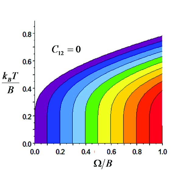
Figure 13: (Color online) Contour plot of thermal pairwise concurrence for field-free case, prepared in same format for comparison with Fig. 8 for the pendular case. Here, $C_{12}(max)$ = 0.1644 at T = 0, $\Omega/B$ = 1.

Figure 13 shows a contour plot of $C_{12}(T)$ for the zero-field case, derived from Eq.(B14). It is qualitatively quite similar to Fig. 8 for the pendular case, over the same wide range of $k_{B}T/B$ and $\Omega/B$.

APPENDIX C: REDUCED VARIABLE FORMULAS

In order to find a proper reduced variable formula, three steps are needed: (1) calculate enough sample points to define well the exact curve; (2) find a function with adjustable parameters that enables fitting those points; (3) evaluate the parameters using a non-linear regression method. For our curve fitting we use the Levenberg-Marquardt Algorithm Kenneth , also called ”Chi-square minimization”. Chi-square is defined as:

$$\chi^{2}=\sum_{i=1}^{N}\left[Y_{i}-f(x_{i};\hat{\theta})\right]^{2}$$ (C1)

where $x_{i}$ and $Y_{i}$ are the independent and dependent variables for the $i^{th}$ (i = 1, 2,…,n) sample points of the exact curve; $\hat{\theta}$ are the parameters to be fitted. The Levenberg-Marquardt algorithm iteratively adjusts the parameters to get the minimum chi-square value, which corresponds to the best fit. The input data for fitting Eqs.($19,22,25,26$) comprised our numerical results for the pendular case, over the ranges $x=\mu$$\mathbf{\varepsilonup}$/$B$ = 0 to 8. Tables III - VI list the optimal values found for the parameters and 95% percent confidence intervals. At $x=0$, the Eq.(19) fit gives $K(0)=0.17103$, different slightly from the exact zero-field limit, $K(0)=1/6$. Likewise, at $x=0$ the Eq.(25) and (26) fits give $C_{0}=0.005$ and $C_{1}=0.00072$ rather than the exact value of zero. The critical point for $C_{1}$ to change sign is $x=4.902$, whereas Eq.(26) gives $C_{1}=-0.00025$, slightly different from zero.

Table 3: Values of the parameters for Eq.(19).

Parameters	Pendular	Field-free	CI
$A_{1}$	0.01092	0.00221	$\pm$0.0003
$A_{2}$	0.21953	0.24779	$\pm$0.006
$x_{0}$	0.96578	0.74035	$\pm$0.05
$\triangle x$	0.97429	0.86072	$\pm$0.03

Table 4: Values of the parameters for Eq.(22).

Parameters	Values	CI
$A_{1}$	12.42379	$\pm$0.0533
$A_{2}$	-10.47646	$\pm$0.0534
$x_{0}$	8.77516	$\pm$0.0534
$p$	1.5867	$\pm$0.00527

Table 5: Values of the parameters for Eq.(25).

Parameters	Values	CI
$A_{1}$	0.84855	$\pm$0.00145
$A_{2}$	-0.84355	$\pm$0.00180
$x_{0}$	1.6339	$\pm$0.00508
$p$	1.2459	$\pm$0.00539

Table 6: Values of the parameters for Eq.(26).

Parameters	Values	CI
$A_{0}$	-0.75212	$\pm$0.0323
$A_{1}$	1.04192	$\pm$0.0336
$A_{2}$	1.14092	$\pm$0.0325
$x_{1}$	-0.16241	$\pm$0.0224
$x_{2}$	3.1232	$\pm$0.124
$\triangle x_{1}$	0.90544	$\pm$0.0136
$\triangle x_{2}$	2.76286	$\pm$0.0496

For convenience, we give formulas for the three unitless ratios, evaluated with customary units:

$\mu$$\varepsilonup$$/B$ = 0.0168 $\mu(Debye)$$\varepsilonup$$(kV/cm)/B(cm^{-1})$;

$\Omega/B=5.04\times 10^{-9}\mu^{2}(Debye)/r^{3}(microns)/B(cm^{-1})$;

$k_{B}T/B=0.695\;T(K)/B(cm^{-1})$.

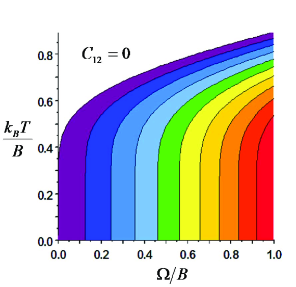
Figure 8: (Color online) Contour plot of thermal pairwise concurrence for two dipoles, for $\mu$$\varepsilonup$$/B$ = 3. For $0<\Omega/B<1$, the maximum concurrence $C_{12}(max)$ = 0.0473, occurs at T = 0, $\Omega/B$ = 1. The plot displays normalized contours. Within each colored band, the variation of $C_{12}/C_{12}(max)$ is 0.1; thus the normalized concurrence in the right most band (red) ranges from 0.9 to 1; in the next band (orange red), from 0.8 to 0.9, etc. A striking feature is the large region (uncolored) where $C_{12}$ = 0. There, entanglement does not occur unless the dipole-dipole coupling exceeds a critical value dependent on the temperature.

References

- (1) D. DeMille, Phys. Rev. Lett. 88, 067901 (2002)
- (2) L. D. Carr, D. DeMille, R. V. Krems and J Ye, New Journal of Physics 11, 055049 (2009).
- (3) R. V. Krems, W. C. Stwalley, and B. Friedrich, Cold molecules: theory, experiment, applications (Taylor and Francis, 2009).
- (4) B. Friedrich and J. M. Doyle, ChemPhysChem 10, 604 (2009)
- (5) C. Lee and E. A. Ostrovskaya, Phys. Rev. A 72, 062321, (2005)
- (6) S. Kotochigova and E. Tiesinga, Phys. Rev. A 73, 041405(R) (2006)
- (7) S. F. Yelin, K. Kirby and R. Cote, Phys. Rev. A 74, 050301(R) (2006)
- (8) A. Micheli, G. K. Brennen and P. Zoller, Nature Phys. 2, 341 (2006)
- (9) E. Charron, P. Milman, A. Keller and O. Atabek, Phys. Rev. A 75, 033414 (2007)
- (10) E. Kuznetsova, R. Cote, K. Kirby and S. F. Yelin, Phys. Rev. A 78, 012313 (2008)
- (11) K. K. Ni, S Ospelkaus, M. H. G. de Miranda, A. Peer, B. Neyenhuis, J. J. Zirbel, S. Kotochigova, P. S. Julienne, D. S. Jin and J. Ye, Science 322, 231 (2008)
- (12) J. Deiglmayr, A. Grochola, M. Repp, K. Mortlbauer, C. Gluck, J. Lange, O. Dulieu, R. Wester and M. Weidemuller, Phys. Rev. Lett. 101, 133004 (2008)
- (13) S. F. Yelin, D. DeMille and R. Cote, Quantum information processing with ultracold polar molecules in [3], p. 629 (2009)
- (14) A. Wallraff, D. I. Schuster, A. Blais, L. Frunzio, R. S. Huang, J. Majer, S. Kumar, S. M. Girvin and R. J. Schoelkopf, Nature 431, 162 (2004)
- (15) A. S. Sorensen, C. H. van der Wal, L. I. Childress and M. D. Lukin, Phys. Rev. Lett. 92, 063601 (2004)
- (16) A. Andre, D. DeMille, J. M. Doyle, M. D. Lukin, S. E. Maxwell, P. Rabl, R. J. Schoelkopf and P. Zoller, Nature Phys. 2, 636 (2006)
- (17) M. A. Nielsen and I. L. Chuang, Quantum Computation and Quantum Information, (Cambridge: University Press, 2000).
- (18) G. Chen, D. A. Church, B. G. Englert, C. Henkel, B. Rohwedder, M. O. Scully, M. S. Zubairy, Quantum Computing Devices: Principles, Designs, and Analysis, (Chapman and Hall/CRC, Baton Roton, 2007).
- (19) T. Siegfried and L. Sanders, Science News 178 15 22 (No. 11, 2010)
- (20) A. Osterloh, L. Amico, G. Falci and R. Fazio, Nature 416, 608 (2002)
- (21) W. Dur, L. Hartmann, M. Hein, M Lewenstein, and H J Briegel, Phys. Rev. Lett. 94, 097203 (2005)
- (22) S. Q. Su, J. L. Song and S. J. Gu, Phys. Rev. A 74, 032308 (2006)
- (23) S. Kais, Adv. Chem. Phys. 134, 493 (2007)
- (24) L. Amico, R. Fazio, A. Osterloh and V. Vedral, Rev. Mod. Phys. 80, 517 (2008)
- (25) V. Vedral, Nature 453, 1004 (2008)
- (26) L. Cincio, J. Dziarmaga, and M. M. Rams, Phys. Rev. Lett. 100, 240603 (2008)
- (27) O. Osenda, Z. Huang and S. Kais, Phys. Rev. A 67, 062321 (2003)
- (28) Z. Huang, O. Osenda and S. Kais, Phys. Lett. A 322, 137 (2004)
- (29) Z. Huang and S. Kais, In. J. Quant. Information 3, 83 (2005)
- (30) Z. Huang and S. Kais, Phys, Rev. A 73, 022339 (2006)
- (31) Q. Xu, S. Kais, M. Naumov and H. Sameh, Phys. Rev. A 81, 022324 (2010)
- (32) Q. Wei, S. Kais and Y. Chen, J. Chem. Phys. 132, 121104 (2010)
- (33) B. Friedrich and D. Herschbach, Z. Phys. D 18, 153 (1991)
- (34) C. Ticknor and J. L. Bohm, Phys. Rev. A 72, 032717 (2005); J. L. Bohm, M. Cavagnero and C. Ticknor, New J. Physics 11, 055039 (2009)
- (35) J. A. Jones, PhysChemComm 11, 1 (2001)
- (36) H. K. Hughes, Phys. Rev. 72, 614 (1947)
- (37) W. K. Wootters, Phys. Rev. Lett. 80, 2245 (1998)
- (38) S. Hill and W. K. Wootters, Phys. Rev. Lett. 78, 5022 (1997)
- (39) We thank an anonymous reviewer for a comment that induced us to bring out this symmetry.
- (40) J. A. Jones and M. Mosca, J. Chem. Phys. 109, 1648 (1998)
- (41) B. Zhou, R. Tao and S. Q. Shen, Phys. Rev. A 70, 022311 (2004)
- (42) S. Lloyd, Science 261, 1569 (1993)
- (43) D. G. Cory, A. F. Fahmy and T. F. Havel, Proc. Natl. Acad. Sci. 94, 1634 (1997)
- (44) Our discussion of the CNOT operation is largely drawn from tutorial instruction kindly given us by D. DeMille, amplifying the discussion of Fig.17.2 in ref. 13.
- (45) C. H. Townes and A. L. Schawlow, Microwave Spectroscopy (McGraw-Hill, New York, 1955)
- (46) S. Kotochigova and D. DeMille, Phys. Rev. A 82, 063421 (2010)
- (47) L. Wharton and W. Klemperer, J. Chem. Phys. 38, 2705 (1963)
- (48) L. Wharton, M. Kaufman, and W. Klemperer, J. Chem. Phys. 37, 621 (1963)
- (49) Our discussion of line widths is based on conversations with W. Klemperer, interpreting observations made in refs. xx and Wharton .
- (50) S. C. Wofsy, J. S. Muenter, and W. Klemperer, J. Chem. Phys. 53, 4005 (1970).
- (51) A. J. Stone, The Theory of Intermolecular Forces (Clarendon Press, Oxford, 2002), p. 40.
- (52) P. Stelmachovic and V. Buzek, Phys. Rev. A 70, 032313 (2004)
- (53) K. Levenberg, Q. Appl. Math. 2, 164 (1944)