Confined gluon from Minkowski space continuation of PT-BFM SDE solution

Abstract

Recent lattice studies exhibit infrared finite effective QCD charges. Corresponding gluon propagator in Landau gauge is finite and nonzero, suggesting a mechanism of dynamical gluon mass generation is in the operation. In this paper, the analytical continuation of the Euclidean (spacelike) Pinch Technique-Background Field Method (PT-BFM) solution of Schwinger-Dyson equation for gluon propagator to the timelike region of $q^{2}$ is found. We found the continuation numerically showing good agreement with a generalized Lehman representation for small Schwinger coupling. The associate non-positive spectral function has an unexpected behavior. Albeit infrared Euclidean space solution naively suggests like single scale ”massive” propagator, the obtained spectrum of gluon propagator does not correspond to the delta function at single scale $q=m$ , instead more possible singularities are generated. The pattern depends on the details of assumed Schwinger mechanism: for stronger coupling there are few maxima and minima which appear at the scale $\Lambda$, while for perturbatively small Schwinger coupling the spectral function shows up two narrow peaks: particle and ghost excitation, which have mutually opposite signs.

I Introduction

Infrared behavior of Green’s functions (GFs) of pure Yang-Mills theories has been intensively studied in the last decade. Even though GFs are gauge fixing dependent objects and thus they do not represent physical observables, it is believed they include reliable nonperturbative information about confinement (and chiral symmetry breaking when quarks are included). Various solutions for GFs have been obtained by solving Schwinger-Dyson equations (SDEs) and by lattice calculations. Recently, study of SDEs offer two scenarios which are distinguished by the infrared behavior of GFs. The so called scaling solution exhibits power law momentum behavior with an infrared exponents LESM2002 ; ZW2002 ; FIPA2007 which lead to infrared vanishing Landau gauge gluon propagator $\Delta(0)=0$ and correspondingly infrared enhanced ghost propagator. For a SDEs treatment in QCD let us refer ROBSCM ; ALKSME2001 .

On the other side, recent lattice calculations BOU2007 ; BLYMPQ2008 ; lat1 ; lat2 ; lat3 ; lat4 ; CUME2008 ; BIMS2009 ; IRITANI ; DUGRSO2008 ; DUOLVA2010 ; BGLYMRQ2010 ; TW2010 in conventional Landau gauge support the so called decoupling solution. In this scenario the gluon propagator $\Delta(0)\not=0$, but stays finite. Also, it is notable, the ghost propagator is not enhanced in the infrared and thus remains semi-perturbative. Such decoupling solutions, called sometimes massive solutions were already proposed in COR1982 ; COR1986 ; COR1989 and being based on attractive theoretical frameworks of Pinch Technique and Background Field Method (PT-BFM) they attract many new attentions these days JHEP ; PENIN ; BIPA2002 ; BIPA2004 ; BIPA2008 ; cornwall2009 ; SA2010 ; AGBIPA2008 ; AGBIPA2011 . Comparing to standard gauge fixed set of GFs it has been proved that using Pinch Technique- one can rearrange usual gauge fixed GFs (in any gauge) in a way that they do not depend on the gauge fixing parameters and PT GFs satisfy original WTI an not more complicates Slavnov-Taylor identities, for the topical review see rewiev2009 . While scaling solution would be compatible with Gribov-Zwanziger confinement scenario, it is believed that the decoupling solutions is related to a dynamical generated gluon mass $m^{2}\simeq\Delta^{-1}(0)$, however confinement mechanism of associated massive gluons remains to be determined.

The truncation of such reorganized SDEs with WTI satisfying internal vertices is called ”PT-BFM inspired” or simply PT-BFM gluon SDE. As a starting point we use the model originally solved in Euclidean space and for certain set of free parameters presented in the paper JHEP . The dynamical mass generation is a BFM generalization of the well known Schwinger mechanism, hereby singular vertex appears in quantum loops only and not due to the Goldstone modes, which do no take place here as the gauge symmetry is exactly preserved. However as we do not solve more complicated SDE for the gluon vertices, we freely accommodate modeled transversal part in its original form JHEP . Having solved the problem in the Euclidean space we formally perform analytical continuation of the equation to the timelike region, i.e. to the Minkowski space, where it should provide analytical continuation as a solution.

In BFM scheme, the expected Schwinger mechanism gives rise to the infrared gluon mass which naively could not be so far from the value of $\Delta^{-1/2}(0)$, while the true physical particle mass is determined as the pole mass of the full propagator. For a stable unconfined particle it can be extracted as a real solution of equation: $\Delta^{-1}(q^{2}=m_{p}(q^{2}))=0$. Gluon is experimentally unobservable as a particle and thus very likely free plane wave solution does not exists. If there is no real pole in the gluon propagator then a propagation of on-shell gluon is indeed impossible. What is the singularity structure of the propagator of expectingly confined excitations has not been known. Instead of this, some attempts to determine (not completely understood) gluon mass scale were performed on various theoretical and phenomenological basis cornwall2009 ; SA2010 ; NATALE ; NATALE2 giving us rough and simplified estimate $m_{g}=\Lambda_{QCD}$.

In this paper we study Minkowski space continuation of already considered PT-BFM solution JHEP ,which although well defined in the entire Minkowski space, was numerically performed in Euclidean space only. In reality, we did not get just one solution of continued PT-BFM gluon SDE but many, among them we have to choose the correct solution. For this purpose it is fully legitimate to check the analytical properties which are equivalent to the analyticity Stieltjes transformable function (generalized Lehman representation). This is fully consistent treatment as the Lehman representation was explicitly used during the derivation of the original Euclidean space SDE. Due to this reason we will abandon all the solutions which largely do not fit dispersion relation dictated by Lehman representation. Optimizing the analyticity as far possible we got a few scenarios, albeit they are quite sensitive to the details of the model. Especially, and quite interestingly it allows to answer what could be a physical mass of the gluon in the pure Yang-Mills theory. Neither we found single solution $\Delta^{-1}(q^{2}=m_{p}^{2})=0$ for some pole mass $m_{p}$. Actually, solutions we have found lie between two extreme cases: first is the solution with two particle like singularities with opposite signs and the second case, where there is no solution for the physical mass shell. In later case the associated spectral function is an oscillatory one with a few number of relatively smooth minima and maxima. The later case we can interpret as a spectrum of confined gluon, while the first kind of solutions is very likely an artifact of approximation made. In both cases the solution suggests the first branch point is located in the origin of complex $q^{2}$ plane.

Our convention for Minkowski metric tensor reads: $g_{\mu\nu}=diag(+1,-1,-1,-1)$. Minkowski momenta are not labeled in our notation, while we always write $E$ when we specify the Euclidean momenta, i.e. for instance $q^{2}_{E}=-q^{2}$ for some spacelike momentum $q$. We use simple letter $d$ for the PT-BFM gluon propagator in Minkowski and $d_{E}$ in Euclidean space, while symbol $\Delta$ is used for a conventional propagator defined in given gauge. In the next Sections II and III we describe necessary ingredients of the original PT-BFM SDE and perform formal ”analytical” continuation. In Section IV we continue with RG improved SDEs for which we present numerical solutions. We discuss what happens to the solutions in various cases, we also discuss necessary amount of numerics, which is the key tool to get a correct and stable results in Minkowski space. In the Section V we mention some outcomes for continuation of the lattice gluon propagator and we conclude and discuss some open questions in Section VI.

II Analytical continuation I, PT-BFM gluon SDE

In quantized gauge theory one needs to fix gauge in order to be able to calculate GFs. Usual approach is Fadeev-Popov FP gauge fixing procedure which makes perturbation calculation particularly feasible, however GFs become gauge fixing dependent. Pinch Technique is the S-matrix based construction of gauge fixing independent GFs. After reorganization of GFs (calculated at any gauge) one get new GFs which satisfy Ward Identities instead of usual more complicated Slavnov-Taylor identities. It has been proved to all order of the perturbation that Pinch Technique is equivalent to the theory quantized by Background Field Method at Feynman gauge. Guiding by the principles of Pinch Technique, the PT-BFM gluon SDE has been recently studied in JHEP ; cornwall2009 .

To get infrared finite gluon propagator (and running coupling), the gluon propagator must loose its perturbative $1/q^{2}$ pole through the Schwinger mechanism in Yang-Mills theory AGBIPA2011 . It underlies on the assumption of infrared singular gluon vertex in a way it leaves polarization tensor transverse (gauge invariant). In this paper we simply use the derived PT-BFM equation in JHEP , where Schwinger mechanism is employed through the simple Ansatz for the improper (two leg dressed) three gluon PT-BFM dressed vertex

$$d(k)\tilde{\Gamma}_{\nu\alpha\beta}(k,q)d(k+q)=\int d\omega\rho(\omega)\frac{1}{k^{2}-\omega+i\varepsilon}\Gamma_{\nu\alpha\beta}^{L}\frac{1}{(k+q)^{2}-\omega+i\varepsilon}+d(k)\tilde{\Gamma}_{\nu\alpha\beta}^{T}d(k+q)\,,$$ (1)

where $\Gamma_{\nu\alpha\beta}^{L}$ satisfies tree level WTI and $d$ is scalar function related to the all order PT-BFM gluon propagator which in Landau gauge reads

$$G^{\mu\nu}=\left[-g^{\mu\nu}+\frac{k^{\mu}k^{\nu}}{k^{2}}\right]d(k^{2})$$ (2)

and satisfies generalized Lehman representation

$$d(k^{2})=\int d\omega\frac{\rho(\omega)}{k^{2}-\omega+i\varepsilon}\,$$ (3)

and $\tilde{\Gamma}_{T}$ is the rest of the three gluon improper vertex which is not specified by gauge invariance. The essential feature of the vertex $\Gamma_{\nu\alpha\beta}$ is that apart the structure dictated by WTI it also includes $1/q^{2}$ pole term which gives rise to infrared finite solution. For this purpose the following form

$$d(k)\tilde{\Gamma}_{T}^{\nu\alpha\beta}(k,q)d(k+q) = \int d\omega\rho(\omega)\frac{1}{k^{2}-\omega+i\varepsilon}\Gamma_{\nu\alpha\beta}^{T}\frac{1}{(k+q)^{2}-\omega+i\varepsilon}\,$$

$$\Gamma^{\nu\alpha\beta}_{T}(k,q) = c_{1}[(2k+q)_{\nu}+\frac{q_{\nu}}{q^{2}}(-2k.q-q^{2})]g_{\alpha\beta}+[c_{3}+\frac{c_{2}}{2q^{2}}((k+q)^{2}+k^{2}))](q_{\beta}g_{\nu\alpha}-q_{\alpha}g_{\nu\beta})\,,$$ (4)

has been proposed in JHEP . This vertex is transverse in respect to $q$ ($q.\Gamma=0$) and it respects Bose symmetry to two quantum legs interchange as its origin is due to the quantum loops. In this respect there are no singularities associated with external gluons, avoiding thus singular footprint in (however perturbative) any S-matrix element.

Finally, after the renormalization, it leads to the following form of linearized SDE in Euclidean space:

$$d_{E}^{-1}(q_{E}^{2})=q_{E}^{2}\left\{K+bg^{2}\int_{0}^{q_{E}^{2}/4}dz\sqrt{1-\frac{4z}{q_{E}^{2}}}d_{E}(z)\right\}$$

$$+\gamma bg^{2}\int_{0}^{q_{E}^{2}/4}dzz\sqrt{1-\frac{4z}{q_{E}^{2}}}d_{E}(z)+d_{E}^{-1}(0)\,$$ (5)

where the second line arises due to the Ansatz for the gluon vertex (II) and $K$ is the renormalization constant. Thus the strength of the dynamical mass generation is triggered through the adopted coupling constants $c_{1},c_{2},c_{3}$ which is fully equivalent to the introduction of (in principle arbitrary) constant $\gamma$ and infrared value $d_{E}^{-1}(0)$ (for completeness recall that in the paper JHEP $d(0)$ has be calculated since one of $c_{i}$ was fixed by hand).

The analytical assumption (3) is the right key for finding a correct continuation in Minkowski space. All the singularity structure is encoded in the distribution $\rho$. Thus if one knows somehow the essential type of singularity (the example is simple, i.e. $\rho=\delta(x-a)$ in this case) then one can estimate the positions of induced singularity structure, e.g. the position of the first branch points (thresholds are examples generated by simple poles of internal propagators). Consequently , after making formal analytical continuation of SDE one can evaluate the imaginary and the real part of propagator function at domain where the function $d$ is continuous. This procedure actually works numerically for the models, where the continuous function part of $\rho$ is smooth enough and associated principal value integrals can be performed with high numerical accuracy, see SAULI for a review. However when the coupling constant is large enough, one is faced to an oscillatory behavior of the spectral function $\rho$ SAUBI ; SAULIJHEP ; KUGO and the SDE as an integral equation for $\rho$ becomes unstable. We found the system of such equations extremely unstable in the case of PT-BFM gluon SDE as well and due to this reason we develop different strategy for this purpose.

Due to a simple linear structure of the SDE (II) the analytical continuation is very straightforward. Recall the definition here

$$d_{E}(q_{E}^{2})=-d(-q^{2})\,\,{\mbox{for}}\,\,q^{2}<0\,\,,$$ (6)

where now $d$ is Minkowski space PT-BFM gluon propagator. Putting $q^{2}_{E}\rightarrow-q^{2}$ and considering positive (timelike) $q^{2}$ continuation we get the SDE for continued gluon propagator:

$$d^{-1}(q^{2})=q^{2}\left\{K+bg^{2}\int_{0}^{q^{2}/4}dz\sqrt{1-\frac{4z}{q^{2}}}d(z)\right\}$$

$$+\gamma bg^{2}\int_{0}^{q^{2}/4}dzz\sqrt{1-\frac{4z}{q^{2}}}d(z)+d^{-1}(0)+i\epsilon\,\,$$ (7)

where the substitution $z\rightarrow-z$ was made and also the both sides were multiplied by $-1$.

While the Eq. (II) is formally identical to its spacelike counterpartner , the main difference should be stressed: The function $d$ on the both sides is complex function, the one on the rhs. of SDE is integrated over the region where all singularities are located. Meaning of Feynman $i\epsilon$ is as usual, it is responsible for the generation of absorptive part of $d$ at the timelike region, however here, we keep it small and finite in our numerical treatment. Having $d$ complex, the equation (II) represents two coupled real equations for an imaginary and the real parts of $d$. Thus the presence of small imaginary is crucial for obtaining a correct Minkowski solution. Clearly switching off imaginary factor we would repeat Euclidean space solution again, albeit now for timelike $q^{2}$. Clearly such solution do not complete the full solution in Minkowski space since the timelike solution of Eq. (II) is purely real and contradicts the assumption made. Also note, such solution has an infrared discontinuity $d^{-1}(0^{+})-d^{-1}(0^{-})=2\Lambda^{2}$ (left limit is the Euclidean) , while for a continuous solution we need to adjust $d^{-1}(0^{+})=-\Lambda^{2}$. At this place, we can mention we have found a real solutions of Eq. (II) for $d^{-1}(0^{+})<0$ , which includes the case $d^{-1}(0^{+})=-\Lambda^{2}$ as well. Up to the later case all of them posses second order discontinuity, while for the choice $d^{-1}(0^{+})=-\Lambda^{2}$ we also got the real solution but with the first order singularity only. Of course, these real solutions cannot be interpreted as the analytical continuation which we are looking for since the reality of $d$ completely contradicts our assumptions. Much interesting for us is the following observation: for mentioned solutions we get the second and the first order singularity respectively, which is located at $q^{2}=0$. It is the motivation to look, if not yet an evidence, for the complex solution with the branch point located at the origin of $q^{2}$ complex plane.

We argue here that the solution of Eq. (II) is not unique, there must be more solutions in addition, at least one is complex and respects Lehman representation and corresponds thus to the continuation to the Minkowski timelike domain of $q^{2}$, this later has the branch point located at the origin of Minkowski $q^{2}=0$. There exist probably more (infinite number is not excluded) solutions in other Riemann sheets if $d$ is a multivaluable analytical functions. The required solution is represented by the function which starts to be complex from the origin in accordance with the introduction of trivial boundary in the integral expression (3). Actually we got numerical evidence for such statement by our numerical search.

Before discussing more details, we improve the linearized SDE in a way it gives correct UV asymptotic behavior, for which case we also present the numerical solution.

III Renormalization group improved gluon SDE

Solving the SDE perturbatively by taking $d(z)\rightarrow 1/z$ one get the correct 1 loop perturbative limit

$$d(x)|_{pert}\rightarrow\frac{1}{x(1+bg^{2}ln(x/\mu^{2})}\,.$$ (8)

However, when solving SDE selfconsistently then the solution of (II) leads to the slower decrement with growing momenta $q^{2}$, instead of log suppression we would get $(1+bg^{2}ln(x/\mu^{2}))^{1/2}$ (see JHEP for the details) behavior of the gluonic form factor, which is believed is the prize of the gauge technique and associated renormalization simplifications.

In order to restore the correct RG behavior of the SDE solution one needs to replace

$$g^{2}d(z)\rightarrow\frac{g^{2}}{g^{2}_{UV}(z)}d(z)$$ (9)

in the integrands of SDE, where $g^{2}_{UV}(z)$ is some function with the perturbation theory running coupling ultraviolet asymptotic.

To accomplish this we take the function $g_{UV}$ in the form

$$g^{2}_{UV}(z)=\frac{1}{bln(e+\frac{z}{\Lambda^{2}})}.$$ (10)

Up to an required asymptotic it is smooth function enough, which ensures unwanted infrared modification of the SDE kernel.

As a first necessary step we obtain the solution of PT-BFM SDE in the spacelike region and we solve the SDE in the Euclidean space. Incorporating substitution (9), fitting the renormalization constant $K=1$ we solved the following equation

$$d_{E}^{-1}(q_{E}^{2})=q_{E}^{2}\left\{K+b\int_{0}^{q_{E}^{2}/4}dz\sqrt{1-\frac{4z}{q_{E}^{2}}}d_{E}(z)\frac{g^{2}}{g^{2}_{UV}(z)}\right\}$$

$$+\gamma b\int_{0}^{q_{E}^{2}/4}dzz\sqrt{1-\frac{4z}{q_{E}^{2}}}d_{E}(z)\frac{g^{2}}{g^{2}_{UV}(z)}+d_{E}^{-1}(0)\,.$$ (11)

As in the previous case of Eq. (II), two parameters stay completely free in given truncation. For simplicity and quite naturally we take the infrared gluon mass identical with $\Lambda_{Q}CD$.

$$d^{-1}(0)=\Lambda^{2}\,.$$ (12)

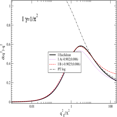
Figure 1: Spacelike solution for the model with coupling $\gamma=1/\pi^{2}$ and $d^{-1}(0^{-})=\Lambda^{2}$. Comparison with spectral representation fits are added, the bracket shows the numerical fit: $(Red(0^{+})^{-1},\epsilon)$ (in units of $\Lambda^{2}$) for which the Minkowski SDE has been solved.

and then looking what happens when $\gamma$ is varied. We have found there is little dependence of the solution even when we change $\gamma$ about order of magnitude, for the solutions see Fig. 1.

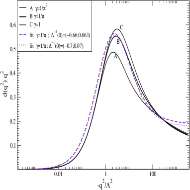
Figure 2: Spacelike solution for various $\gamma$. Dashed and dotted lines represent two fits obtained for $-\gamma=1/\pi$ from Minkowski SDE solution (see the text for the details). The fits are labeled by values of $Red(0^{+})^{-1},\epsilon$ in units of $\Lambda^{2}$.

After a slight rearrangement, the RG improved PT-BFM SDE (III) has been solved by the iteration. The iteration procedure shows up very fast convergence, providing 20-30 iteration steps are enough to achieve vanishing difference between the two followed iterations. Since the Euclidean correlator is quite smooth function thus the resulting solutions are numerically stable. Thanks to the 1-dimensionality of the problem we can use a grid with large number of mesh points giving easily 3 to 6 digit accuracy without a special treatment of the upper boundaries for which we use simple step function. In our treatment we do not define a new gluon form factor neither gluon dynamical mass as this cannot be done without ambiguity. In figure 1 we plot the resulting solution for the dressing function $F=q^{2}d$. The comparison with the 1-loop perturbative running coupling asymptotic is shown in figure 2.

IV Analytical Continuation II, Results for Renormgroup Improved PT-BFM SDE

If gluon were a stable massive particle we could get delta distribution $\delta(\omega-\mu^{2})$ as a first substantial singularity in gluon spectral function. Further there could be a second singularity at $4\mu^{2}$ where the continuous part of spectra usually starts. As the massless ghosts were omitted we could get further singularities at $9\mu^{2},16\mu^{2},...$ all these singularities exhibit ourself as a finite cusps in the real part of $d$, since $\rho$ has no derivatives at these points and all of them could be located on the cut in complex plane which is identical with the real positive semiaxis of Minkowski $q^{2}$.

However, instead of dealing with stable vector particle, we are dealing with confined gluon field. Let us imagine a process when ”high energy” gluon is emitted with some virtuality $q^{2}$. It starts to loose its energy through the pair creation and bremsstrahlung of soft gluons, all these colored intermediate states are finally (and simultaneously) neutralized in a color singlet glueballs (hadrons, when real QCD with quarks is considered). Such color neutralization can happen only through the interaction with other colored partons- gluons and quarks. Gluon never escapes as a free on shell particle, no matter what the typical gluon mass scale would be. From this picture it is apparent: the timelike structure can be quite complicated as many ”intermediate states” contributes significantly because of strong coupling. The emission and absorption of quanta of the fields are related with threshold singularities when unconfined particles are considered. Here, for the case of gluons, we expect something similar, but perhaps qualitatively different: the absorption and emission of confined object could reflect their short life $t\simeq 1/\Lambda_{QCD}$ , we expect this reflection is encoded in the singularity structure typical for confinement. Thus considering spectral function one can really expect kind of cusps instead of delta function and some more smooth non-monotonic behavior instead of threshold cusps. Constrained by construction here, we do not expect their positions in a complex plane away from a positive real axis.

In any case, assuming spectral function has a continuous part we must get standard dispersion relation for

$$Red(k^{2}) = P.\int d\omega\frac{\rho(\omega)}{k^{2}-\omega}\,,$$

$$Imd(k^{2}) = -\pi\rho(k^{2})\,,$$ (13)

where P. stand for principal value integration.

Without knowledge of branch points and singularities in $\rho$ one is faced with problem of performing limiting analytical continuation to the borderline of analyticity- to the cut, where at (hopefully) isolated points we assume $d$ has aforementioned singularities of not yet specified type. Not necessarily but likely, they can be related with a branch points of multivaluable analytical function and very likely the number of them increases with growing $q^{2}$. It is our assumption that all the information about singularities is correctly captured in Minkowski space continued SDE for gluon. Of course , one can expect that various approximation, which are necessary complements of given truncation of SDEs system has an impact on the solution, e.g. on the position, number of branch points and even the analyticity can be destroyed. Finally remind the well known examples: this is the Dirac delta function in spectrum which implies pole in the propagator, similarly Heaviside step function $\theta(x-a)$ gives $log(q^{2}-a)$ divergence and for instance $\theta(1-T/x)\sqrt{(}1-T/x)$ gives usual particle production threshold at $T$. That it is easy to write down a plethora of arbitrarily moderated singularities, which are not familiarly known from particle physics is quite obvious.

In previous discussion we offer some arguments which are crucial for the method of the solution. Let us summarize and specify our assumptions to the following points: 1) Solution for a complex arguments $q^{2},Im\,q^{2}\not=0$ is given by analytical continuation of Euclidean solution. 2) Minkowski solution corresponds with $Im\,q^{2}=0$, which is in principle obtainable by limiting procedure based on (1), can be directly obtained from continued Euclidean SDE, i.e. singularities are integrable and isolated. 3) The first singularity of the gluon propagator is located at the origin of complex plane.

Continuation of PT-BFM gluon SDE is straightforward as there is only function $g$ added when compared to the previous case. First let us rewrite Euclidean SDE by using Minkowski conventions $q^{2}_{E}=-q^{2}$

Following the convention $q^{2}_{E}=-q^{2}$ for negative spacelike Minkowski $q^{2}=q^{2}_{0}-{\bf{q^{2}}}$ then we can rewrite the Eq. (III) like

$$d_{E}^{-1}(-q^{2})=-q^{2}\left\{K+b\int_{0}^{-q^{2}/4}dz\sqrt{1+\frac{4z}{q^{2}}}\frac{d_{E}(z)}{g^{2}_{E}(z)}\right\}$$

$$+\gamma b\int_{0}^{-q^{2}/4}dzz\sqrt{1+\frac{4z}{q^{2}}}\frac{d(z)}{g^{2}_{E}(z)}+d_{E}^{-1}(0)\,,$$ (14)

which is valid for negative $q^{2}=q^{2}_{0}-{\bf{q^{2}}}$. The continuation $d(q^{2})=-d_{E}(-q^{2}_{E})$ to positive $q^{2}$ then reads

$$d^{-1}(q^{2})=q^{2}\left\{K+b\int_{0}^{q^{2}/4}dx\sqrt{1-\frac{4x}{q^{2}}}\frac{d(x)}{g^{2}_{c}(x)}\right\}$$

$$+\gamma b\int_{0}^{q^{2}/4}dxx\sqrt{1-\frac{4x}{q^{2}}}\frac{d(x)}{g^{2}_{c}(x)}+d^{-1}(0)+i\epsilon\,,$$ (15)

i.e. now the integral domain on the rhs. of (II) becomes purely timelike as the all arguments appearing in SDE are. Again we have performed the substitution $x=-z$ in order to show formal similarity with the Euclidean equation. The function $g_{c}$ in Eq. (IV) should be the analytical continuation of our UV renormgroup improver, for which we take the function

$$g^{2}(z)=1/bln(e+|q^{2}|/\Lambda^{2})$$ (16)

where $e=2.73..$ and we neglected $i\pi$ term as a legitimate simplification valid at ultraviolet.

Here we briefly mention trivial fact that the Eq. (IV) includes unphysical solutions, e.g. the real solution $d(z)=d_{E}(z)$, which corresponds to the choice $d^{-1}(0)=d_{E}^{-1}(0)$. We have also found some real solutions even for more ”correct” choice $d^{-1}(0)<0$. Again, they are clearly not hot candidates for wanted analytical continuation, as they do not agree with the dispersion relation (3).

We solve the Eq. (IV) numerically at positive semiaxis $q^{2}=(0,+\infty)$ by the method of iterations. We were searching for complex $d$ which can have nonzero imaginary part everywhere at $R^{+}$. Numerically we take $\epsilon$ as constant satisfying $\epsilon<<|d(0^{+})|$ for all values of $q^{2}$. Numerically, $\epsilon$ must be taken nonzero in order to accurately perform numerical integration in the vicinity of branch points in $d$. A bit unexpectedly a wide variety of stable numerical solutions of Eq (IV) has been found.

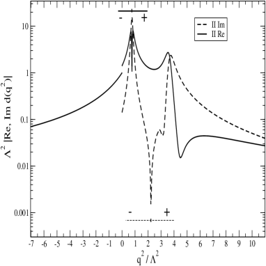
Figure 3: Magnitude of PT-BFM gluon propagator in whole Minkowski space for $\gamma=1/\pi$ and $Red(0^{+})^{-1}=0.7\Lambda^{2}$, $Imd(0^{+})^{-1}=0.07\Lambda^{2}$, $d^{-1}(0^{-})=\Lambda^{2}$).

We anticipate here, the main feature of the solution is the appearance of two relatively large peaks with mutually opposite signs (see the results in figures 3-5) . Such singularities and the associated oscillations make the appropriate numerical findings a really hard problem. We achieve stable numerics by using Gaussian integrators such that intercept between two neighborhood points is smaller then $\epsilon$ in the vicinity of singularities. We found advantageous to iterate not the function $d$, but rather its inverse which leads to very fast numerical convergence. Quite independently on the initial guess, typically $\simeq$ 30-40 iterations are enough to get vanishing $(10^{-15})$ difference between last iterations. For instance the curves shown in Fig 2. were evaluated for 9000 Gaussian mesh points.

In Euclidean space, the value of BFM gluon propagator at zero momenta represents a free parameter which must be fitted by hand. The value $d_{E}(0)=\Lambda$ was chosen for simplicity. There is no free choice when dealing with the SDE in Minkowski space and the right limit of $d$, ie. $d(0^{+})$ value is necessarily constrained by global analytical property of $d$ (stress here , we assume $q^{2}=0$ is a branch point, in principle we allows the left and the right limit differ). Here we describe the numerical treatment which has been actually used in this paper.

To find the best analytical continuation, we scan the values $d(0^{+})$ and $\epsilon$, such that $\epsilon/d(0^{+})<<1$ and $d(0^{+})\simeq(0^{-})=\Lambda$, for each set we find the solution of Minkowski SDEs. Then we check the dispersion relation for the solution $Red(q^{2})$ and $Im\,d(q^{2})$. The one which best reproduce the Euclidean solution via assumed dispersion relation for $d$ is called the best analytical continuation (in sense of the point (2)). In accordance with spectral representation one expects vanishing imaginary part at the infrared as the correct analytical continuum limit. We can conclude, that within an accuracy limited by finite size of $\epsilon$ one can always find the solution of timelike SDE. We expect the numerical accuracy of SDE solution is driven by the ratio, i.e $\epsilon/\Lambda\simeq 0.1-1\%$, while the agreement with assumed analyticity is a different issue. For this purpose we qualify the quality of analytical continuation by evaluating the following difference:

$$\sigma(q^{2})=q^{2}_{E}\left(d_{E}(q_{E}^{2})-\frac{1}{\pi}\int d\omega\frac{-Imd(l^{2})}{q^{2}_{E}+l^{2}}\right)\,$$ (17)

where $d_{E}$ is the numerical solution of (III) and $d$ is the numerical solution of (IV). The best analytical approximation was achieved by minimizing $\sigma$ and thus getting a few percentage deviation (for almost all $q^{2}$) at the minimum. For instance, for the case of small Schwinger coupling $\gamma=0.1$, the best analytical infrared fit we were able to trigger numerically uses $\epsilon=10^{-3}\Lambda^{2}$ while keeping $Re\,d(0^{+})\simeq d_{E}(0)=\Lambda^{2}$. Let us stress the estimate of the numerical systematical error $\simeq 10^{-3}$ (for absolute values of $d$) is always much smaller that the deviations from analyticity which can be estimated approximately by $(d_{E}(0)-d(0^{+}))/(d_{E}(0)+d(0^{+}))\simeq 0.1$ in the infrared.

V $\gamma$ dependence of Minkowski solution

The parameters $\gamma$ represents the strength of the effective coupling constant which arise due to the Schwinger mechanism. Thus numerical value of $\gamma$ should be responsible for the size of $d(0)$ which can be estimated by the feedback of SDE solutions. Therefore we consider several values of $\gamma$ and report numerical results here for small $\gamma=1/\pi^{2}$ and ”large” $\gamma=\pm 1/\pi$ couplings respectively.

In previous section we described the search of continued solution in details. In all studied cases we have found that the agreement with the exact analyticity is somehow limited ( $\sigma=0$ in the exact case). For a larger $\gamma$ it was difficult to get stable solution and minimize $\sigma$ so we were limited by concerning values $|\gamma|<1$. A few examples of a backward analytical continuation are shown in figure 1 for $\gamma=1/\pi^{2}$ and in figure 2 for $\gamma=-1/\pi$, where they are compared with the original Euclidean solutions. Following the numerical procedure described, we label various solutions by the pair of numbers $(Re\,d^{-1}(0^{+}),\epsilon)$ in the units of $\Lambda$. The difference between two initial choices $(-0.902;0.006)$ and $(-0.9025;0.006)$ exhibits numerical sensitivity in the case of small $\gamma$.

While the dependence on $\gamma$ is rather mild in the case of the Euclidean solutions, we have found that this is not the case of the Minkowski space solutions. The solutions show up several cusps, number of them and their shapes largely change when varying $\gamma$. The only approximate invariant is the fact that the first maximum is positive (in sense of spectral function $\rho$) and located more or less at $\Lambda$, while the second peak is negative with the position shifted slightly to a higher scale. Other local maxima and minima are generated as well, also the discontinuity in the first derivatives are found. The first peak is located at scale $\Lambda$, which is in fact our choice of the infrared value of the gluon propagator, and quite expectingly, when the it is sharp enough, then one can see associated quasithreshold (at the scale $2\Lambda$). The second peak is a surprise of the Minkowski solution. For a large momenta $q^{2}>>\Lambda^{2}$ the second singularity regulates the contribution from the first one. Such screening is actually very large for small Schwinger coupling Considering the approximation $\rho(\omega)=\delta(\omega-\mu_{1}^{2})-\delta(\omega-\mu^{2})$ of the infrared spectral function, the screening of the first peak by the second one is obvious. For instance for small $\gamma=1/\pi^{2}$ we have found the position of the peaks are $\mu_{1}\simeq\Lambda,\mu_{2}\simeq\sqrt{2.5}\Lambda$.

In order to get some feeling how the numerical solution depends on the details which are not theoretically fully determined, we modify two parameters in the solely Minkowski SDE (IV), then after getting the solution we again use dispersion relation for $d$ and see how the Euclidean solution is recovered. The main purpose to do this is to see whether the approximation employed has crucial influence on the analyticity. As a first, we have changed the sign of $\gamma$ in the Minkowski SDE and then compare obtained solution with the original Euclidean one via backward continuation (17). However alternating sign of $\gamma$ is ad hoc here, there exists a good motivation: beyond our truncation the constant $\gamma$ will be replaced by the product of vertex function for glueball-like BSE for the gluon vertex. We expect , such product substantial changes when going to Minkowski timelike axis- it becomes complex and very likely enhanced there- therefore alternating the sign may not be so radical for our rough estimate. Actually, as we have found the deviations from analyticity $\sigma$ reaches smaller minima, such scenario is possible and perhaps preferred when compared to the case when $\gamma$ is unchanged. The resulting numerical solution are labeled as Model II in all presented figures, while what is labeled by letter I is calculated without any changes. Also the fits in figure 2 are based on the backward continuation of Minkowski solutions II which are displayed in figures 3-5.

Secondly, we slightly change the improver $g_{c}$, again solely in Minkowski SDE. For this purpose we replace the Euler constant $e$ in the expression (16) by free parameter $C$. As a result, we have found $g_{c}$ enhanced (taking $C=2.5$) is numerically preferred for positive value of $\gamma$, while taking $g_{c}$ slightly suppressed (taking $C=3.5$) we can get better fits of Euclidean solution for negative $\gamma$. As an effect these changes modify the shape of the peaks. The appropriate solution for $\gamma=1/\pi$ coupling is added in figure 4. As one can see the second peak quite changes not only position but it transforms to a much narrower cusp. From this one can conclude that the analytical form of the resulting Minkowski propagator can be quite sensitive to the numerical approximations, which can be only marginal in the Euclidean treatment.

As one can see from the Figs. 4 and 5, taking $\gamma$ small one get the solution with two very narrow peaks located at few $\Lambda^{2}$. We could expect these peaks should be visible in a hadronic S-matrix element whenever timelike gluon is interchanged as an intermediate excitation. There would be ”long living gluon” and ”long living gluonic ghost” at the scale $\Lambda$ according to their numerical ”widths” which has the size by order smaller then $\Lambda$. Disregarding the reality of such scenario, we get interesting solution-two possible excitations appear for a single field $A$. Let us imagine what happens when we collide hadrons in such a world. Whenever energetically possible the quarks (and gluons itself) would preferably exchange low energy gluons with positive virtuality corresponding to the singularities or maxima positions and such peaks of gluonic colored corellator will become visible through the color subchannels. Even after the integration over the distribution of quarks, such gluonic colored mediators would be observed as resonances with very large cross sections (although without any doubt we know that many gluon interchanges are necessary to describe hadronic amplitudes, as only very large number can be responsible for formation of hadronic resonances, for very nice illustration see the study MARCOT2002 on $\pi-\pi$ scattering).

Increasing $\gamma$ changes the shape of the gluon propagator, especially the sharp peaks are melted down as they are transformed into more smooth maxima. For large $\gamma$ this is the branch point in the origin which is sole numerically observed singularity of the gluon propagator. The details of melting peaks is nicely seen in figure 5.

VI Fitting the lattice

The framework of PT-BFM SDEs is based on well defined theoretical background and in principle it could finally provide a gauge fixing independent set of new Greens functions. Nevertheless, the quantitative comparison with the standard-gauge fixed lattice simulation is further stimulating. Actually, there is small quantitative difference between decoupling Euclidean solutions, and the lattice evaluation of gluon propagator in Landau gauge AGBIPA2008 ; AGBIPA2010 ; BI2010 . In this respect, the analytical continuation obtained from PT-BFM SDE can be regarded as an reliable estimate of Minkowski space continuation of lattice data.

Based on suitable numerical fits at Euclidean regime, a various form of continuation were proposed for scaling solutions of SDEs Alkofer . According to the conclusion and numerical findings in Alkofer , the singularities of scaling solution studied are located near the real timelike semiaxis of the momenta. It is quite likely that the qualitative analytical properties of various solutions of YM SDEs systems are frankly insensitive to finiteness of $d(0)$ and thus both, the scaling and the decoupling solutions of gluon propagators can be captured by the formula for Lehman representation. Then the quantitative difference will result from different forms of $\rho$, whatever it could be. Recent lattice data show finite infrared gluon propagator, which however is usual property of massive propagator, but as we have shown it does not necessary mean propagation of massive particle. There are legitimate attempts to move the first branch point towards the higher timelike scale SUGANUMA ; IRITANI , which fits are based on low $q^{2}$ lattice data. The first singularity fitted in this way assume quite obscured form of the spectral function. It is taken as a product of delta function and the inverse square root function singular at the point. Although it allows a reasonable estimate of the singularity position $m=600MeV$ and it provides rough numerical fit of the Euclidean data at the region 0.5-5 GeV , the choice of the singularity form is far from obvious. The other lattice fits were proposed in the literature. For instance in the papers DUGRSO2008 ; DUOLVA2010 the function

$$\Delta(k^{2})=\frac{k^{2}+M^{2}}{k^{4}+(M^{2}+m^{2})k^{2}+\lambda^{4}}\,$$ (18)

was used to describe the lattice prediction for the infrared gluon propagator up to $k\simeq 1.5GeV$. The function $\Delta$ has two complex conjugated poles and thus certainly does not belong to the sort of functions satisfying dispersion relation (3). However, as it was shown recently in DUDAL2011 , when $\Delta$ is considered in the loop, the resulting expression can be cast into the form of Eq. (3) (in fact, it is kind of an evidence, that albeit $D$ does not have Lehman representation, its inverse has a part, which after the renormalization can be expressed through the dispersion relation).

In our case, we have an additional hint estimated from the behavior of SDEs solution: the PT-BFM gluon propagator posses the first branch point at $q^{2}=0$ and the others are generated on the real axis by the Gauge Technique construction and selfconsistently determined by solving the continued SDE (IV). Making backward analytical continuation we reproduce the Euclidean solution approximately. From this we know, that we did not cross any singularities when one deforms usual Wick rotation contour at $q_{0}$ plane. This is a strong argument which supports our findings, when comparing for instance to ad hoc guess of the singularity structure from fitting of shape of the Euclidean lattice data.

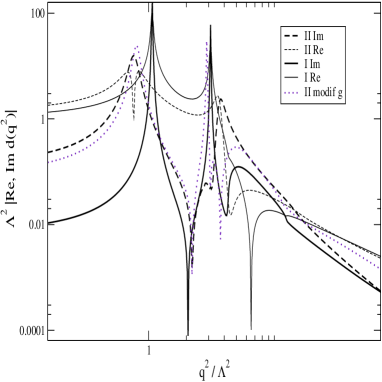
Figure 4: Magnitude of PT-BFM gluon propagator in Minkowski space for Model I: $\gamma=1/\pi^{2}$ and $Red(0^{+})^{-1}=0.9\Lambda$, $\epsilon=0.006\Lambda^{2}$, corresponding $d^{-1}_{E}(0)=\Lambda^{2}$ and the Model II, which is the same as in the Fig. 3. Dotted lines represents Model II but with the function $g_{c}$ as described in the text.

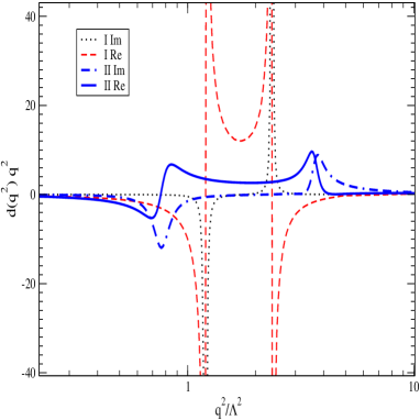
Figure 5: Details of the singularities (and shape) of the timelike gluon form factor as obtained for small $\gamma=1/\pi^{2}$ (Model I) and moderate coupling $\gamma=1/\pi$ (Model II) respectively.

VII Conclusion

The main purpose of our paper is to show that Stieltjes transformation or equivalently generalized Lehmann representation exists for PT-BFM gluon propagator. Very likely, the same applies for the conventional Landau gauge gluon propagator recently seen in the lattice simulation. We have found reliable spectral function for all $q^{2}$, not only at the infrared or ultraviolet part separately. According to the expectations, the gluon propagator exhibits violation of positivity. In accordance with confinement the main singularity does not correspond with single delta function. However, for a small coupling characterizing the strength of the YM Schwinger-mechanism the infrared gluon propagator can be approximated by two mutually opposite sign Yukawa propagators, while the whole propagator function needs a certain amount of the continuous background in addition. Increasing $\gamma$ we get a more realistic picture of confinement -the sharp peaks in spectral function are melted down, while the Lehman approximation is less approximative, perhaps showing the evidence for complex conjugated poles of the from (18). According to our approximative findings, the continuous spectrum starts at zero momenta, where we expect the first branch point. For small $\gamma$ , this is in excellent agreement with the assumption: the propagator is finite and purely real at light cone $q^{2}=0$. However for a larger $\gamma$ we get small imaginary part, which contradicts coexistence of Lehman representation and finiteness of the real part of gluon propagator at zero momenta. This, although small discrepancy tell us that our analytical assumption is not fulfilled , but is justified as an approximation only.

In order to discuss a possible sources of this discrepance let us tentatively divide the gluon PT-BFM propagator into two peaces:

$$d(q^{2})=\int d\omega\frac{\rho(x)}{q^{2}-x+i\varepsilon}+r_{NA}(q^{2})\,,$$ (19)

where $r_{NA}(q^{2})$ should be small when compared to the full $d(q^{2})$ and we distinguish among several possibilities.

1. where $r_{NA}$ is the marginal complex remnant which does not obey Stieltjes representation but does not contradict Wick rotation and thus the primacy of Euclidean calculation as well. The example is complex pole located at point $z$ with $Rex>0$ and $Imz<0$

2. $r_{NA}$ does not allow Wick rotation, there are singularities and cuts in complex plane of $q^{2}$ (and $q_{0}$) which makes the theories in Euclidean and Minkowski space different. In this case, the lattice data should be regarded as a certain approximation of Minkowski spacelike correlators. The example of such behaviour we can mention is the function given by (18), if it has complex pole at some $z,Rez>0,Imz>0$.

3. $r_{NA}$ vanishes for the full solution. It is possible it is a consequence of approximation employed, eg. it is a possible artifact of weakness of the Gauge Technique linearization, truncation of SDE system, modeling Schwinger mechanism and modeling UV RG improver $g_{c}$. In this case the idea of analytical effective charge finds new applications beyond its original perturbative conjecture SHIRKOV ; MISO1997 ; MISO1998 ; SHISOL2007

To distinguish among above three points is beyond our recent analyzing power, however in future study one should always ask, what improvement of the knowledge has been achieved in this respect.

In practice, most of theoretical description of QCD processes is based on the factorization schemes where the hard part of amplitudes is calculated by using perturbation theory while the non-perturbative information is included in the partonic distribution functions. Therefore the first hint we can get, can be obtained from the phenomenological studies which adopt the running charges constrained by finite BFM gluon propagator, for recent calculation of the proton structure function see NATALE , and NATALE2 for heavy meson decay study. The timelike gluons exchanged certainly appear in the s-channel of meson scattering or heavy meson strong decays. The calculation difficulty of such process is obvious, the observed gluon peaks will interfere not only with itself, but with the first colorless resonances, e.g. $\rho$ meson which always arise nonperturbatively when very large number (infinite) gluons are exchanged (MARCOT2002 ). Nevertheless the difficulty of the problem, we believe that propagator calculated here can be useful when one would like to investigate glueball and hadron spectra in cases when timelike kinematics is especially pronounced. For this purpose inclusion of the quark fields remains to be done.

References

- (1) C.Lerche, L. von Smekal, Phys. Rev. D65,125006 (2002).
- (2) D. Zwanziger, Phys. Rev. D65 094039 (2002).
- (3) C.S. Fischer, J.M. Pawlowski, Phys. Rev. D75,025012 (2007).
- (4) C.D. Roberts, S.M. Schmidt, Prog.Part.Nucl.Phys. 45, (2000).
- (5) R. Alkofer, L. Smekal, Phys.Rept. 353 (2001).
- (6) Ph. Boucaud et all., Eur. Phys. J. A31 ,750, (2007).
- (7) Ph. Boucaud, J-P. Leroy, A. Le Yaouanc, J. Micheli, O. Pene, J. Rodriguez–Quintero, JHEP0806, 012 (2008).
- (8) A. Cucchieri, T. Mendes, PoSLAT2007, 297 (2007).
- (9) A. Cucchieri, T. Mendes, Phys. Rev. Lett. 100 241601, (2008).
- (10) Ph. Boucaud, J.P. Leroy, A. Le Yaouanc, J. Micheli, O. Pène, J. Rodríguez-Quintero, JHEP0806, 099 (2008).
- (11) O. Oliveira and P. Bicudo, arXiv:1002.4151 [hep-lat].
- (12) A. Cuchieri and T. Mendes, Phys. Rev. Lett. 100 241601, (2008).
- (13) I.L. Bogolubsky, E.M Ilgenfritz, M. Muller-Preussker and A. Sternbeck, Phys. Lett. B676,69 (2009).
- (14) T.Iritani, H.Suganuma, H.Iida, Phys. Rev. D80,114565, (2009).
- (15) D. Dudal, J.A. Gracey, S.P. Sorella, N. Vandersickel and H.Verschelde, Phys. Rev. D 78, 065047 (2008).
- (16) D. Dudal,O. Oliveira and N. Vandersickel, Phys. Rev. D 81 074505 (2010).
- (17) Ph. Boucaud et all, Phys. Rev. D82, 054007 (2010).
- (18) M.Tissier and N. Wschebor, Phys. Rev. D 82, 101701 (2010).
- (19) J.M. Cornwall, Phys. Rev. D26,1453 (1982).
- (20) J. Cornwall and W.S. Hou, Phys. Rev. D34 585, (1986).
- (21) J. Cornwall and J. Papavassiliou, Phys. Rev. D40 3474, (1989).
- (22) A.C. Aguilar, J. Papavassiliou, JHEP0612:012, (2006).
- (23) M.R. Pennington, talk at International Workshop on Effective Field Theories: from the pion to the epsilon,Valencai 2009, arXiv:0906.106.
- (24) D. Binosi, J. Papavassiliou, Phys.Rev. D66, 111901 (2002) .
- (25) D. Binosi, J. Papavassiliou, J.Phys. G30, 203 (2004)
- (26) D. Binosi, J. Papavassiliou, JHEP0811, 063 (2008).
- (27) D. Binosi, J. Papavassiliou, Phys. Rep. 479, (2009).
- (28) A. C. Aguilar, D. Binosi, J. Papavassiliou, Phys. Rev. D78: 025010, (2008).
- (29) J. M. Cornwall, Phys. Rev. D80, 096001 (2009).
- (30) V.Sauli at EXCITEDQCD2010 Stara Lesna, arXiv:0906.2818, On the decoupling solution for pinch technique gluon propagator.
- (31) E.G.S. Luna, A.A. Natale, A.L. dos Santos, Phys. Lett. B698, 52 (2011).
- (32) C. M. Zanetti, A. A. Natale arXiv:1007.5072.
- (33) L.P.Fadeev, V.N. Popov, Phys. Lett. B25, 29 (1967).
- (34) V. Sauli ,FewBodySyst. 39, 45 (2006).
- (35) V. Sauli, J. Adam, P. Bicudo, Phys. Rev. D75, 087701 (2007).
- (36) R. Fukuda and T. Kugo, Nucl. Phys. B 117 250, (1976). Schwinger-Dyson equation for massless vector theory and Absence of fermion pole.
- (37) V. Sauli, JHEP 0302, 001, (2003).
- (38) S. R. Cotanch, P. Maris, Phys. Rev. D66,116010 (2002).
- (39) H.Suganuma, T.Iritani,A,Yamamoto, Lattice QCD Study for Gluon propagator and Gluon Spectral Function, PoS QCD-TNT09, 044 (2009); arXive:10011.0007
- (40) D. Dudal and M.S. Guimaraes, Phys. Rev. D83, 045013 (2011).
- (41) A. C. Aguilar, D. Binosi, J. Papavassiliou, arXiv:1004.1105.
- (42) D. Binosi, at Light Cone 2010: Relativistic Hadronic and Particle Physics, 14-18 June 2010, Valencia, arXiv:1004.1105.
- (43) A. C. Aguilar, D. Binosi, J. Papavassiliou, arXiv:1107.3968.
- (44) R. Alkofer, W. Detmold, C. S. Fischer, P. Maris, Phys. Rev. D70, 014014 (2004)
- (45) D.V. Shirkov, I.L. Solovtsov, Phys, Rev. Lett. 79, 1209 (1997).
- (46) K.A. Milton, I.L. Solovtsov, Phys. Rev. D55, 5295, (1997).
- (47) K.A. Milton, O.P. Solovtsova, Phys. Rev. D57,5402 (1998).
- (48) D. V. Shirkov, I. L. Solovtsov, Theor. Math. Phys. 150, 132 (2007).