KA-TP-06-2011
Light Stop Decay in the MSSM with Minimal Flavour Violation
M. Mühlleitner and E. Popenda
Institut für Theoretische Physik, Karlsruhe Institute of Technology, 76128 Karlsruhe, Germany
Abstract
In supersymmetric scenarios with a light stop particle and a small mass difference to the lightest supersymmetric particle (LSP) assumed to be the lightest neutralino, the flavour changing neutral current decay can be the dominant decay channel and can exceed the four-body stop decay for certain parameter values. In the framework of Minimal Flavour Violation (MFV) this decay is CKM-suppressed, thus inducing long stop lifetimes. Stop decay length measurements at the LHC can then be exploited to test models with minimal flavour breaking through Standard Model Yukawa couplings. The decay width has been given some time ago by an approximate formula, which takes into account the leading logarithms of the MFV scale. In this paper we calculate the exact one-loop decay width in the framework of MFV. The comparison with the approximate result exhibits deviations of the order of 10% for large MFV scales due to the neglected non-logarithmic terms in the approximate decay formula. The difference in the branching ratios is negligible. The large logarithms have to be resummed. The resummation is performed by the solution of the renormalization group equations. The comparison of the exact one-loop result and the tree level flavour changing neutral current decay, which incorporates the resummed logarithms, demonstrates that the resummation effects are important and should be taken into account.
1 Introduction
The Standard Model (SM) provides a very successful effective theory of
particle interactions which is in excellent agreement with electroweak
precision data. Furthermore, remarkable consistency and precision
tests have been made in the sector of quark flavour violation.
These tests and limits on flavour changing neutral currents (FCNC) from
and studies put strong constraints on possible New
Physics beyond the SM [1]. They forbid a generic
flavour structure of New Physics at the TeV scale and raise the
question why contributions from New Physics at TeV are
strongly suppressed. A solution to this
New Physics Flavour Puzzle is provided by the framework of Minimal
Flavour Violation (MFV)
[2, 3, 4, 5].
It requires all sources of flavour and CP-violation to be given by the
SM structure of the Yukawa couplings. Flavour mixing in models of New
Physics is then always proportional to the off-diagonal elements of the
Cabibbo-Kobayashi-Maskawa (CKM) matrix [6].
In particular, the mixing of the third generation squarks with the first and
second generation squarks is highly suppressed by small CKM quark
mixing angles.
Since the flavour structure of New Physics at the TeV scale must be
non-generic, flavour measurements provide a good probe of New
Physics. One of the best studied examples is given by
supersymmetry (SUSY). In the context of flavour violation the
phenomenology of the light stop partner is especially
interesting. In most SUSY models a light stop quark mass
arises naturally. Due to the large top Yukawa coupling the mixing
between the weak eigenstates and leads to
a large mass splitting between the stop mass eigenstates. Furthermore,
the large top Yukawa coupling in general drives the stop mass via the
renormalization group equation (RGE) running to smaller masses, even
if all squarks have a common mass at the SUSY breaking scale. In
scenarios with a light stop which predominantly decays into a
charm quark and the lightest neutralino, assumed to be the
lightest supersymmetric particle (LSP), , squark flavour violation can be tested by
exploiting stop decay length measurements [7]. It has been
shown, that in these scenarios light stops can be discovered at the
LHC [8]. Finally, a light stop is also favoured by baryogenesis
which requires a stop mass with about the top mass value or less for
successful electroweak baryogenesis within the context of the Minimal
Supersymmetric Extension of the Standard Model (MSSM) [9].
Minimal Flavour Violation naturally arises in supergravity models
which provide flavour-independent scalar mass terms at a high
scale like the Planck scale . Some time ago the authors of
Ref. [10] have provided an approximate formula for
the flavour changing neutral current (FCNC)
decay by starting from a
vanishing tree level coupling at the
Planck scale. The decay then proceeds via one-loop diagrams. The
non-vanishing divergences, which are due to scalar self-mass diagrams,
have been subtracted by a soft counterterm at the Planck scale so that
a large logarithm remains at the weak scale chosen
to be . The authors argue that in view of this large logarithm,
the remaining non-logarithmic part of the one-loop diagrams can hence
safely be neglected so that their result for the decay width takes a
rather simple form.
In this work, we perform the complete one-loop calculation of the
decay in the framework of MFV. We
perform the full renormalization program and keep the finite
non-logarithmic terms arising from the loop integrals.
This allows us to study the importance of the neglected
non-logarithmic pieces in the formula given by Ref.[10].
To get a reliable result, the appearing large logarithms should be
resummed. In the renormalization group approach this corresponds to
solving the renormalization group equations for the scalar soft SUSY
breaking squark masses. As has been pointed out in
[4], the hypothesis of MFV is not renormalization
group invariant. Flavour off-diagonal squark mass terms are hence
induced by the Yukawa couplings, so that the squark and quark mass
matrices cannot be diagonalized simultaneously any more and the stop
state receives some admixture from the charm squark, inducing a FCNC
between stop, charm and LSP neutralino,
. From this point of view, the
logarithmic piece of our one-loop result is equivalent to the first order in the
expansion of the RGE solution for the squark-quark-neutralino coupling
in powers of , whereas the tree level decay calculated
with the FCNC coupling includes the resummation of the large
logarithms. The comparison of the two decay widths provides an
estimate of the importance of the resummation of the large
logarithms.
The outline of our paper is as follows: In section 2 we present the diagrams contributing to the one-loop decay. We set up our notation for the squark and quark sector in section 3. The counterterms and the renormalization are discussed in section 4. Section 5 contains the numerical analysis. We conclude in section 6. In the Appendix we list our Feynman rules, the various amplitudes contributing to the decay and we derive the FCNC counterterm.
2 One-loop decay
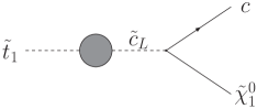

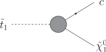
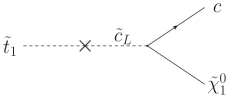
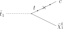
We work in the framework of the MSSM with MFV so that all flavour changing effects with quarks and squarks are controlled by the quark Yukawa couplings and CKM mixing angles [3]. The decay of the lightest stop into the lightest neutralino and a charm quark ,
| (1) |
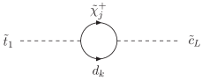
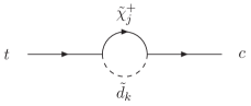
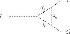
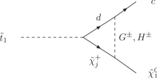
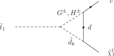
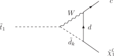
is then mediated at the one-loop level. We consider scenarios where the light stop is the next-to-lightest supersymmetric particle (NLSP) and the lightest neutralino is the LSP. The process is built up by the stop and charm self-energies and the vertex diagrams, cf. Fig. 1. Note, that in our calculation we set
| (2) |
Therefore in the self-energies we have only non-vanishing contributions for transitions into the left-handed charm squark . Those into right-handed scharm, , are zero for . All diagrams are mediated by charged current loops. The various diagrams which contribute are depicted in Fig. 3. The self-energies and vertex corrections are divergent and have to be renormalized. The counterterms for the squark and quark self-energies and for the vertex renormalization are shown in Fig. 3.
![]()
![]()


![]()
![]()
![]()


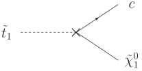
The FCNC
vertex does not arise at tree level. Its occurrence as counterterm at
one-loop level is due to the fact that MFV is not RGE-invariant,
since the weak interactions affect the squark and quark mass matrices
differently [11]. Their simultaneous diagonalization
cannot be maintained at higher orders so that it can consistently be
imposed at a single scale only, called
in the following.
For the calculation of the stop decay process we define an effective interaction vertex
| (3) |
where denote the charm and neutralino spinors and are the four-momenta of the outgoing neutralino and charm quark. and are form factors associated with the chirality projectors and , respectively. They receive contributions from the vertex diagrams, from the quark and squark self-energies, and from the vertex and the quark and squark wave function renormalization counterterms,
| (4) |
They are specified in section 4 and the Appendices B1-3 and C.
3 The quark and squark sector
For the choice of our notation the quark and squark sectors are discussed here in more detail. The definition of the couplings is deferred to Appendix A. We define the unitary matrices as the matrices which rotate the left- and right-handed up- and down-type quark current eigenstates to their corresponding mass eigenstates, ,
| (5) |
The CKM matrix is given by
| (6) |
For the squark interaction eigenstate we define a six component vector
| (9) |
where are each a three component column vector in generation space. The squared squark mass matrix can be written as a Hermitian matrix of blocks
| (12) |
It is diagonalized by a unitary matrix which rotates the squark interaction eigenstates to their mass eigenstates ,
| (13) |
The six component column vector is defined to be ordered in mass, with being the lightest squark. Equation (13) can then be rewritten as
| (14) | |||||
where denotes the generation index.111We have thus decomposed the mass eigenstate squark field into left- and right-chiral interaction eigenstate squarks. The rotation of the squarks by the same unitary matrices as the quarks defines the super-CKM basis. In models with non-minimal flavour violation the squark mass matrix is flavour-mixed in this basis, in contrast to the quark mass matrix. In models with MFV at the scale , however, the squarks can be rotated by to their flavour eigenstates in parallel to the quarks, and the super-CKM basis is at the same time the flavour eigenstate basis. Hence, suppressing generation indices,
| (15) |
The squared mass matrix in the flavour eigenstate basis then reads
| (18) |
where for down- and up-type squarks. With we denote the ratio of the vacuum expectation values of the two complex Higgs doublets. They are introduced in order to generate masses of up- and down-type fermions [12]. The parameter denotes the trilinear coupling of the soft SUSY breaking part of the Lagrangian, the Higgsino mass parameter and the quark partner mass. is a unit matrix in generation space. The parameters are given by the left- and right-handed scalar soft SUSY breaking masses and the -terms,
| (19) |
where denotes the third component of the weak isospin, the electric charge, the boson mass and the Weinberg angle. The squared mass matrix can be diagonalized by a unitary matrix which rotates the flavour eigenstates to their mass eigenstates,
Comparison with Eqs. (14) and (15) shows that we can factorize the matrices into the flavour-diagonal matrices and the quark rotation matrices defined above,
| (23) |
with . The matrix can be expressed in terms of mixing angles by
| (24) |
For the three quark generations the relation between the flavour eigenstates and the squark mass eigenstates hence reads
| (25) |
For better legibility, we suppress the generation indices from now on wherever possible, and the lighter and heavier squark mass eigenstates are generically called and . The mixing angles are then given by
| (26) |
and the masses of the squark mass eigenstates read
| (27) |
Since the mixing angles are proportional to the masses of the quarks, the mixing is important in the stop sector and can drive the lightest stop mass even lighter than the top quark mass.
4 Counterterms and Renormalization
The quark and squark self-energies and the vertex diagrams are ultraviolet (UV) divergent and need to be renormalized. The quark and squark wave functions are renormalized on-shell. With the bare (s)quark fields () related to the renormalized (s)quark fields () by
| (28) |
this leads for the squarks to the following off-diagonal elements of the wave function renormalization constants in terms of the real part of the squark self-energy ,
| (29) |
Defining the following structure for the quark self-energy,
| (30) |
we have for the corrections to the off-diagonal chiral components of the quark wave functions,
| (31) | |||||
As for our scenario we chose the to be the NLSP, all our self-energies are real, and after the on-shell renormalization of the quark and squark wave functions we are only left with the one-loop vertex diagrams and the FCNC vertex counterterm. From now on “Re” will be dropped. We regularize the divergences by dimensional regularization in dimensions so that ultraviolet singularities appear as poles in . We have explicitly verified that the same result is obtained with dimensional reduction. By exploiting the unitarity relations of the CKM matrix as well as those of the chargino mixing matrices and , defined in Appendix A, we find for the vertex contribution to the form factors
| (32) | |||||
| (33) |
where denotes the ’t Hooft mass of dimensional regularization. We have used the short-hand notation
| (34) |
where denote matrix elements of the
matrix, which diagonalizes the neutralino mass matrix, cf. Appendix A.
The further ’finite terms’ in Eq. (32), which do not
depend on , can be extracted from the full one-loop
result for the vertex which is given in Appendix B3. We have
introduced a generic mass for the loop particles, . Note, that in the numerical analysis we will use the
exact results with the different loop particle masses. Here, for
reasons of legibility and also to make later contact with the result
derived in Ref. [10] we adopt the generic notation. The
left-handed form factor is zero due to our choice of vanishing
-quark mass.
The FCNC counterterm arises from the flavour non-diagonal part of the wave function renormalization, from the renormalization of the quark and squark mixing matrices [13, 14, 15, 16] and the renormalization of the quark masses.222In our renormalization procedure and the definition of the counterterm we follow the same approach as in Ref. [17]. The renormalized squark mixing matrix is related to the bare by
| (35) |
And similarly, the renormalized quark mixing matrices are related to the bare quark matrices by
| (36) |
The indices denote the six squark mass eigenstates, and are generation indices. We impose the MFV condition on the renormalized mixing matrices and hence demand them to be flavour diagonal. This leads to flavour non-diagonal counterterms . Furthermore, as the bare and renormalized mixing matrices are unitary the counterterms must be antihermitian. The UV divergent part of each counterterm is determined such that it cancels the divergent part of the antihermitian part of the corresponding wave function renormalization matrix [14, 15, 16],
| (37) | |||||
| (38) |
The general form of the FCNC vertex counterterm depicted in Fig. 3 has been derived in Appendix C. For our process we have the following form factor contributions to the vertex counterterm,
| (39) | |||||
| (40) |
with
| (41) |
and
| (42) | |||||
| (43) |
The squark wave function has been renormalized at . The finite parts of the counterterms Eqs. (37,38) depend on the renormalization conditions. Absorbing also the finite part of the antihermitian wave function renormalization leads to a gauge-dependent on-shell renormalization scheme [16, 15, 18]. Performing minimal subtraction on the other hand is gauge-independent [19] and imposes the MFV condition on the parameters at the scale . In the following we will adopt this scheme. Consequently, the result will depend on the MFV scale . The squark mixing matrix counterterm then reads333This counterterm definition can lead to large contributions to the matrix element if . For a discussion, see e.g. Refs. [20]. In the scenarios of our numerical analysis we have .
| (44) |
A gauge invariant prescription for the quark mixing matrix counterterm is given by [15],
| (45) |
For the quark mixing matrix contribution to the vertex counterterm we then find
| (46) |
For the contribution from the squark mixing we have
| (47) |
with
| (48) |
It depends on the Higgsino parameter , the soft SUSY breaking
mass parameter including term
contributions, the trilinear coupling , the
mixing angle , the boson mass and the pseudoscalar Higgs mass
.
The contribution from is given by
| (49) |
As before, we have introduced a generic loop particle mass, and ’finite terms’ denote further terms which do not depend on . Their specific form can be extracted from the explicit formulae of the stop self-energies given in Appendix B1. Inserting Eqs. (42,46,47,49) in Eq. (39), the right-chiral part of the FCNC counterterm is then given by
| (50) |
Adding Eqs. (32) and (50) and replacing and by Eq. (34) and Eq. (48), respectively, we arrive at the following final result for the form factors, which contribute to Eq. (4),
| (52) |
Finally, the stop decay width in terms of the form factors Eqs. (4,52) is given by
| (53) |
As can be inferred from , depending on the scale of MFV, the logarithm can become very large, and the decay can become important in certain regions of the parameter space, especially for large values of . The finite terms, which do not depend on , are then only subleading. If we drop the finite terms in Eq. (4), the approximate result given by Hikasa and Kobayashi in Ref. [10] should be reproduced. In fact, for we can rewrite
| (54) |
where denotes the mass parameter of the Higgs doublet which couples to down-type fermions. With this relation the form factor Eq. (4) leads to the approximate result of Ref. [10], if we set the MFV scale equal to the Planck scale, , choose as generic loop particle mass and neglect the finite terms,
| (55) | |||||
In our full one-loop calculation of the decay width in terms
of , Eq. (4), the finite terms are included,
and the relevance of these contributions can
be checked by comparing with the approximate result for
the decay width in terms of the form factor ,
Eq. (55). This will be discussed in section
5.
To get a reliable result, the large logarithms of the MFV scale in the
decay formula should be resummed. The logarithm is related to the
running of the FCNC coupling of the neutralino to a quark and squark
of different generations. We have required this coupling to vanish at the scale
. Minimal Flavour Violation is not
RGE-invariant, however. Even though MFV is imposed at
, at any other scale a FCNC coupling will be generated
through renormalization group evolution. The solution of the one-loop
RGE for the quark and squark mixing matrices provides the resummation
of the large . The coefficient of
this logarithm in
Eq. (4) is then given by the first order in the
expansion of the RGE solution for the squark-quark-neutralino coupling
in powers of . In the following we will call the right-handed
form factor including the resummation effects . It is
given by the FCNC coupling obtained through renormalization group evolution
including flavour violation of the squark and quark mixing matrices,
from some high scale down to the scale relevant for the decay process.
5 Numerical Analysis
The scenarios for the numerical analysis have been chosen such that they lead to a NLSP stop and a LSP. The latter represents a promising dark matter (DM) candidate in the MSSM [21]. The mass difference is chosen to be small enough so that the loop mediated flavour changing decay is dominating and can compete with the four-body decays444Scenarios where 2-body decays at tree level are forbidden for the lightest stop quark and where the loop induced flavour changing decay competes with 3-body decays have been discussed in [22]. into the LSP, a -quark and a fermion pair [23],
| (56) |
Such scenarios can be consistent with electroweak baryogenesis
[9] and
also with Dark Matter constraints [24]. The mass spectra
and mixing angles have been calculated with the spectrum calculator SPheno
[25] and compared to SOFTSUSY [26].
Both codes include the option to perform two-loop RGE running with and
without the inclusion of flavour violation and both support the
SUSY Les Houches accord [27]. Within this accord the
gauge and Yukawa couplings as well as the soft SUSY breaking mass
parameters and trilinear couplings are given out as
running parameters at a scale , which we
have chosen to be the scale of electroweak symmetry breaking
(EWSB). We have verified that the calculation
of the decay width leads to the same result if we apply dimensional
reduction instead of dimensional regularization, so that the
running parameters can be used.
The mixing matrix elements and the SUSY particle pole masses
have been taken at the scale of EWSB as well. The SM parameters have
been chosen as GeV,
,
,
GeV,
GeV and
GeV. We have chosen the CKM matrix elements as and .
In order to ensure MFV, for all three generations a common mass parameter
for the soft SUSY breaking masses of the
doublet has to be introduced at the scale , so that the up- and down-type squark mass matrices can be
simultaneously flavour-diagonal. We work in the framework of a MFV
MSSM defined at the GUT scale in terms of a small number of
parameters. They are given by common soft SUSY breaking scalar
and gaugino mass terms, and , a common SUSY breaking
trilinear coupling , the ratio of the two vacuum expectation
values and the sign of the Higgsino parameter
.
5.1 Analysis for GeV
We first investigate two mSUGRA scenarios with soft-breaking terms at the GUT scale GeV, which is identified with the MFV scale. All soft SUSY breaking parameters are family universal. The boundary conditions at are
| (61) |
The second scenario has a larger mass difference compared to scenario (1), whereas the mass difference between and the lightest chargino is smaller. Since the 4-body decays are dominated by the chargino exchange diagram [23], in scenario (2) the 4-body decays should be more important leading to a smaller branching ratio of the flavour changing decay. The GUT scale is given by GeV. The masses are obtained by RGE evolution from the GUT scale down to the electroweak scale. The running is performed at two-loop order without the inclusion of explicit flavour violation in the squark sector. The obtained masses are
| (64) |
For these scenarios the partial stop decay width into charm and neutralino, calculated with the full one-loop formula, is compared to the approximate result. For the latter, we take as generic loop particle mass, cf. Eq. (55). The widths and form factors are given in Table 1. They have been obtained with the program SUSY-HIT [28], where the full one-loop formula for the flavour changing stop decay has been implemented.
As can be inferred from the table, the exact and approximate decay
width differ by %. In fact, the finite terms
extracted from the one-loop formula turn out to contribute with % to , Eq. (4). This difference leads to
the 10% effect in the decay width. The difference in the branching ratio
calculated in the two
approaches is negligible, however. We note, that in the first scenario the partial
width is times smaller than in the second scenario due the smaller
mass difference and hence reduced phase
space.
For the calculation of the branching ratios, also the partial
width for the decay into -quark and neutralino,
, as well as the 4-body decay width
are needed. The former is suppressed by 2 orders of magnitude compared
to the final state due to the small CKM matrix
element which enters quadratically in
the decay width. The branching ratios are listed in Table 2. As
anticipated, the stop 4-body decay is more important in scenario (2)
leading to a change of the branching ratio of interest,
, at the few per-cent level.
As stated before, the large logarithms in the decay formula should be resummed. To get an estimate of the importance of the resummation effects, the one-loop decay calculated in the framework of MFV is compared to the tree level stop decay into charm and neutralino with flavour off-diagonal elements in the squark mixing matrix. They are the result of the small flavour off-diagonal entries introduced in the soft-breaking terms through RG evolution including the complete flavour structure of the different flavour matrices, from the scale of MFV down to the scale of EWSB. The input parameters for the decay formula are taken from SPheno [25]555Thanks to Werner Porod who provided us with the newest SPheno version 3.0.beta56.. In the flavour violating case, denoted by FV in the following, where no flavour-eigenstates exist any more, the lightest up-type squark state has been identified to correspond to . The scenarios in Eq. (61) have been chosen such that . The and masses are almost unchanged. The form factor of the tree level decay is given by the right-handed part of the FCNC coupling666The left-handed part is negligibly small for .,
| (65) |
with the squark mixing matrix defined in Eq. (14). This leads to the partial decay width
| (66) |
The form factors and partial widths are shown in Table 3. As can be inferred from the table, there is a factor between the right-handed form factor calculated at the one-loop level in the MFV framework and the one derived from RG evolution including flavour
violation. As expected, resummation effects turn out to be important for a
large scale 777This result is in agreement with the discussion in
Ref. [29] where resummation effects in the coupling
have been found to be large..
The partial widths, which depend quadratically on the right-handed
form factor, differ by a factor .
For comparison we have performed the calculation with the decay
spectra and mixing angles evaluated by SOFTSUSY. The squark mixing
matrix elements agree within accuracy with the results of
SPheno. The mixing matrix element ,
which enters in the form factor
Eq. (65), is and differs in the two
spectrum calculators. The two codes implement the one-loop corrections
to the squark mass matrices differently. SOFTSUSY corrects only the
flavour-diagonal entries of the squark mass matrices, while SPheno
implements a full one-loop calculation, so that differences in the
flavour off-diagonal entries are to be expected. For the SOFTSUSY
parameter values, this results in a ratio between loop decay and tree
level decay of for the two scenarios, compared to the
ratio found with the SPheno parameter values. All in all,
the results with both spectrum calculators show the importance of the
resummation effects.
Of phenomenological interest are the consequences of these resummation effects on the branching ratio into the charm plus neutralino final state. To quantify this, the competing 4-body stop decay width, calculated in the FV scenario and including tree level FCNC couplings, is needed. The additional FCNC contributions are expected to be small, however, due to the suppression by CKM matrix elements. As the calculation is not available at present we defer a detailed comparison to a future publication.
5.2 Analysis for
In the previous section the importance of resummation effects has been discussed. With decreasing and hence smaller on the other hand the non-resummed one-loop MFV result should approach the resummed flavour-violating tree level result. Furthermore, we expect the approximate formula of Ref. [10], which is a good approximation of the exact one-loop MFV result for large scales, to be less good with decreasing MFV scale. In order to verify this behaviour we have chosen scenarios with different varied between GeV. We choose the soft SUSY breaking input parameters888In our scenarios varies between 10 and 20. in each scenario such that the masses for and remain almost unchanged. Consequently, the differences in the partial decay widths will not be due to phase space effects. Furthermore, the scenarios are constrained by the requirement that is the NLSP and is the LSP, so that the FC decay dominates. The relevant particle masses for the different scenarios vary as
| (67) |
with the mass difference ranging between
| (68) |
We emphasize that the following results are purely
illustrative. The various scenarios have not been required to fulfill
Dark Matter constraints and/or constraints from electroweak precision
data. The
main emphasis was to achieve approximately constant masses for the
NLSP and LSP.
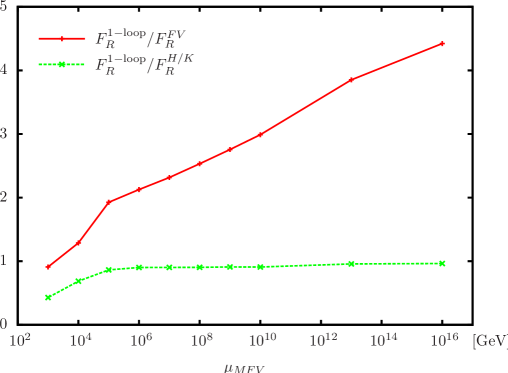
In Fig. 4 we show, as a function of the MFV scale, the
ratio of the non-resummed right-handed form factor
in the MFV 1-loop decay to
in the FV tree level decay as well as
the ratio of to the approximate form
factor .999Note that the line
connecting the different points uniquely serves to guide the eye.
As can be inferred from the
figure, the approximate result reproduces the one-loop result down to
low scales. Starting from GeV
the finite terms become relevant. At GeV neglecting the finite terms in
leads to a factor between the
approximate and the 1-loop form factor. The
non-resummed 1-loop result and the resummed tree level result, on the
other hand, approach each other with decreasing scale of MFV as
expected.
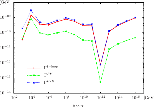
Figure 5 shows the partial widths as functions of
for the approximate MFV decay, for the
full MFV 1-loop decay and for the tree level resummed decay.
An interesting feature which can be inferred from
Fig. 5 is the size of the decay width. It does not
only depend on the size of the logarithm but also on the coefficient
of the logarithmic term, which is given in terms of the soft SUSY
breaking parameters, particle masses and mixing angles, cf.
Eq. (4). As explained above, for each value of the
scale we have chosen a different set of
boundary conditions such
that the and masses remain
approximately unchanged. This leads for each to a different coefficient of the logarithmic term. For
GeV e.g. the parameter
set and resulting masses and mixing angles are such that the
coefficient becomes rather small, so that the partial width is less
than GeV. Due to the large value of the logarithmic contribution still dominates over the
finite terms, however, so that there is good agreement between the 1-loop and
approximate result. For small values of the partial width can be as large as a few GeV as
the factor, which multiplies the logarithm, turns out to be large for
the chosen parameter set. The value of the coefficient is also the reason for
the kink in Fig. 4 at GeV.
Figure 5 shows, that in
accordance with the behaviour of the right-handed form factors, at
high scales the 1-loop and the approximate result agree up to the
effect of the non-logarithmic terms on the partial width, which is at the
10% level. The 1-loop and the resummed tree level
decay agree at low scales where the resummation effects of the large
logarithms can be neglected, whereas the deviations are large for high
scales. In summary, in order to get correct predictions for the
flavour changing light stop decay for large scales of MFV, resummation
effects have to be included. To further improve on this decay, the
next step is the calculation of the one-loop corrections to the tree
level stop decay including the squark mixing matrix elements from RGE
evolution. This is deferred to a future publication.
6 Summary and Conclusions
In summary, we have calculated the flavour violating decay in the framework of Minimal Flavour Violation including also finite terms, which do not depend on the logarithm of the MFV scale . The one-loop decay has been compared to the approximate result derived earlier by Hikasa and Kobayashi which neglects the subleading terms compared to the large logarithm of . It has been found that it approximates the complete one-loop result within 10% for large MFV scales. The approximation becomes worse with decreasing scales. The one-loop result, and also the approximate formula, however, do not resum the large logarithms. The resummation is done by solving the renormalization group equations. Since MFV is not RG-invariant, flavour changing off-diagonal elements are induced in the squark mixing matrices which lead to FCNC couplings at tree level. They can be compared to the effective one-loop coupling in the MFV approach. The resummation effects turn out to be important, so that the one-loop result and the formula by Hikasa and Kobayashi only give an approximate value of the phenomenologically important light stop decay width into charm and neutralino. The next important step to improve the prediction for the light stop decay width will be the calculation of the one-loop corrections to the flavour-violating tree level decay.
Appendix
A Couplings
To set up our notation for the couplings, we briefly repeat the chargino and neutralino systems. The chargino mass matrix, in terms of the wino mass parameter , and , is given by [30]
| (71) |
where denotes the charged boson mass and we use , . It is diagonalized by two real matrices and ,
| (74) |
with the Pauli matrix rendering the chargino masses positive. are rotation matrices with the mixing angles
| (75) |
The two chargino masses read
| (76) |
The four-dimensional neutralino mass matrix in the basis has the form
| (81) |
with . It can be diagonalized
analytically [31] with a single matrix .
In the following, we list the couplings in the framework of MFV
[30, 32, 33, 34],
which are
needed for our calculation. All couplings are normalized to the weak
gauge coupling if not stated otherwise. Note that all charged
couplings involving quarks and/or squarks have to be multiplied with the CKM
matrix element , which we have factored out from our
definition of the couplings.
The couplings of charginos and neutralinos to the charged gauge bosons :
| (84) |
The couplings of charginos and neutralinos to charged Higgs
and Goldstone bosons101010We work in the
Feynman gauge.,
, :
| (87) |
| (90) |
The couplings between neutralinos, quarks and squarks, :
| (97) | |||||
| (104) |
with and for up- and down-type quarks, and
| (105) |
where .
The couplings between charginos, quarks and squarks,
, for up- and down-type
(s)quarks read
| (112) | |||||
| (117) |
| (124) | |||||
| (129) |
The couplings of the gauge bosons, the charged Higgs
and Goldstone bosons to quarks
are given by
| (130) |
| (131) |
| (132) |
The couplings of the gauge bosons and charged Higgs
and Goldstone bosons to squarks
are given by
| (135) |
| (136) | |||||
where
| (137) | |||||
And for the Goldstone couplings we have
| (138) | |||||
and
| (139) | |||||
For our calculation we also need the 4-squark coupling between stop, scharm and two identical down-type squarks. With the generation index and the index denoting the two down-type squark eigenstates, it reads in terms of
| (140) |
and
| (146) |
The couplings with two squarks are obtained from those
with the squarks by interchanging .
Finally, the couplings between stop, scharm and two charged Higgs bosons or two charged Goldstone bosons in terms of are given by
| (147) |
and
| (148) |
where
| (151) |
B1 Squark self-energy contributions
In this Appendix we give the result for the self-energy in terms of the couplings defined in Appendix A. The self-energy receives contributions from the various diagrams in Fig.3, i.e.
| (152) |
Note that the self-energy for and external legs is zero for vanishing quark mass,
| (153) |
We have for
| (154) | |||||
with etc. given in Eq. (117). The sum is taken over the chargino eigenstates and the three quark generations. The scalar one-loop one- and two-point integrals and are defined as [35]
| (155) | |||||
| (156) |
Note the suppression by the CKM matrix elements , . We find for :
| (157) |
The sum is to be taken over the three squark generations and the two squark mass eigenstates . The Goldstone contribution reads
| (158) |
and the self-energy involving the boson
| (159) | |||||
Finally, we have the tadpole contributions from the charged Higgs and Goldstone boson loop,
| (160) |
and the one from the 4-squark vertex
| (161) |
B2 Quark self-energy
According to the structure of the quark self-energy given in Eq. (30) we find for the left-chiral contribution
| (162) | |||||
with given in Eq. (129). The sums are taken over all possible chargino states (), the three quark and squark generations () and the two squark mass eigenstates (). Furthermore, in terms of the scalar one- and two-point functions is given by
| (163) |
The right-chiral contribution reads
| (164) | |||||
with defined in Eq. (129). It vanishes for . The left-chiral scalar contribution can be cast into the form
| (165) | |||||
which also vanishes for zero charm quark mass. For the right-chiral scalar contribution we find
| (166) | |||||
Note that in case of real two-point functions we have .
B3 Vertex correction
The vertex contributions to the left-chiral form factor vanish for . For the right-chiral form factor they are given by the various right-chiral contributions from the vertex correction graphs depicted in Fig.3
| (167) | |||||
We have for ,
| (168) | |||||
where the sum over all possible chargino eigenstates (), all three generations of down type quarks and squarks () as well as the two squark mass eigenstates () has to be taken. We have introduced the abbreviations
| (171) |
with the various couplings defined in Eqs. (104,117,129). The scalar one-loop 3-point function is given by
| (172) |
We find
| (173) | |||||
with
| (175) |
Note that we set the down and strange quark mass to zero, . We have
| (176) | |||||
where
| (178) |
And
| (179) | |||||
with
| (182) |
Next
| (183) | |||||
and
| (184) | |||||
Furthermore,
| (185) | |||||
with
| (186) |
and
| (187) | |||||
with
| (188) |
We have
| (189) | |||||
And finally
| (190) | |||||
with
| (191) |
C FCNC counterterm
We start from the neutralino part of the Lagrangian in the interaction basis, expressed in terms of the bare squark and quark fields, and and the bare quark mass matrix , where denote the generation indices and the neutralino mass eigenstates,
| (192) | |||||
The couplings have been defined in Eq. (105). Let us look at the right-chiral part of the coupling. Rotation to the mass eigenstates yields
| (193) | |||||
Note, that , , cf. Eq. (14). Upon renormalization we replace [16]
| (194) | |||||
| (195) | |||||
| (196) |
where we have suppressed the indices. The wave function denotes a six-component column vector. With the replacement , cf. Eq. (23), we have for the Yukawa part of the coupling
| (197) |
times . For the mass renormalization we choose the renormalization prescription such that the bare mass matrices and hence are diagonal, i.e.
| (198) |
where denotes diagonal matrices. This is possible since the off-diagonal elements can be absorbed into the off-diagonal elements of the antihermitian part of the right-handed wave function renormalization matrices [36]. Exploiting the unitary of the mixing matrices we finally find for the renormalized Lagrangian in the mass eigenstate basis
| (199) |
with the couplings given by
| (200) | |||||
| (201) | |||||
| (202) | |||||
| (203) | |||||
In the framework of MFV at the matrix is diagonal in flavour space at tree level. At one-loop flavour off-diagonal elements are induced through the wave function and the mixing matrix renormalization.
Acknowledgments
We greatly acknowledge helpful discussions with Ben Allanach, Andreas Crivellin, Manuel Drees, Bastian Feigl, Jaume Guasch, Jong Soo Kim, Ulrich Nierste, Werner Porod, Heidi Rzehak, Pietro Slavich and Michael Spira. We are grateful to Ulrich Nierste, Pietro Slavich and Michael Spira for the careful reading of the manuscript. This research was supported in part by the Deutsche Forschungsgemeinschaft via the Sonderforschungsbereich/Transregio SFB/TR-9 Computational Particle Physics. EP gratefully acknowledges support of the Graduiertenkolleg “High Energy Physics and Particle Astrophysics”.
References
- [1] A. Masiero, O. Vives, Ann. Rev. Nucl. Part. Sci. 51 (2001) 161 [hep-ph/0104027]; Y. Grossman, Z. Ligeti and Y. Nir, Prog. Theor. Phys. 122 (2009) 125 [arXiv:0904.4262 [hep-ph]]; G. Isidori, Y. Nir, G. Perez, [arXiv:1002.0900 [hep-ph]].
- [2] R. S. Chivukula, H. Georgi, L. Randall, Nucl. Phys. B292 (1987) 93; L. J. Hall, L. Randall, Phys. Rev. Lett. 65 (1990) 2939.
- [3] A. J. Buras, P. Gambino, M. Gorbahn, S. Jager and L. Silvestrini, Phys. Lett. B 500 (2001) 161 [arXiv:hep-ph/0007085].
- [4] G. D’Ambrosio, G. F. Giudice, G. Isidori and A. Strumia, Nucl. Phys. B 645 (2002) 155 [arXiv:hep-ph/0207036].
- [5] C. Bobeth, M. Bona, A. J. Buras, T. Ewerth, M. Pierini, L. Silvestrini and A. Weiler, Nucl. Phys. B 726 (2005) 252 [arXiv:hep-ph/0505110].
- [6] N. Cabibbo, Phys. Rev. Lett. 10 (1963) 531; M. Kobayashi and T. Maskawa, Prog. Theor. Phys. 49 (1973) 652.
- [7] G. Hiller and Y. Nir, JHEP 0803 (2008) 046 [arXiv:0802.0916 [hep-ph]]; G. Hiller, J. S. Kim and H. Sedello, Phys. Rev. D 80 (2009) 115016 [arXiv:0910.2124 [hep-ph]].
- [8] T. Han, K. i. Hikasa, J. M. Yang and X. m. Zhang, Phys. Rev. D 70 (2004) 055001 [arXiv:hep-ph/0312129]; S. Kraml, A. R. Raklev, Phys. Rev. D73 (2006) 075002 [hep-ph/0512284]; S. Bornhauser, M. Drees, S. Grab and J.S. Kim, [arXiv:1011.5508 [hep-ph]].
- [9] M. S. Carena, M. Quiros, C. E. M. Wagner, Phys. Lett. B380 (1996) 81 [hep-ph/9603420] and Nucl. Phys. B524 (1998) 3 [hep-ph/9710401]; B. de Carlos, J. R. Espinosa, Nucl. Phys. B503 (1997) 24 [hep-ph/9703212]; P. Huet, A. E. Nelson, Phys. Rev. D53 (1996) 4578 [hep-ph/9506477]; D. Delepine, J. M. Gerard, R. Gonzalez Felipe et al., Phys. Lett. B386 (1996) 183 [hep-ph/9604440]; M. Losada, Nucl. Phys. B537 (1999) 3 [hep-ph/9806519] and Nucl. Phys. B569 (2000) 125 [hep-ph/9905441]; V. Cirigliano, S. Profumo, M. J. Ramsey-Musolf, JHEP 0607 (2006) 002 [hep-ph/0603246]; Y. Li, S. Profumo, M. Ramsey-Musolf, Phys. Lett. B673 (2009) 95 [arXiv:0811.1987 [hep-ph]]; V. Cirigliano, Y. Li, S. Profumo et al., JHEP 1001 (2010) 002 [arXiv:0910.4589 [hep-ph]]; M. Carena, G. Nardini, M. Quiros et al., JHEP 0810 (2008) 062 [arXiv:0806.4297 [hep-ph]] and Nucl. Phys. B812 (2009) 243 [arXiv:0809.3760 [hep-ph]].
- [10] K. i. Hikasa and M. Kobayashi, Phys. Rev. D 36 (1987) 724.
- [11] J. F. Donoghue, H. P. Nilles, D. Wyler, Phys. Lett. B128 (1983) 55.
- [12] P. Fayet, Nucl. Phys. B 90 (1975) 104, Phys. Lett. B 64 (1976) 159 and Phys. Lett. B 69 (1977) 489; S. Dimopoulos and H. Georgi, Nucl. Phys. B 193 (1981) 150; N. Sakai, Z. Phys. C 11 (1981) 153; K. Inoue, A. Kakuto, H. Komatsu and S. Takeshita, Prog. Theor. Phys. 67 (1982) 1889, ibid. 70 (1983) 330, ibid. 71 (1984) 413.
- [13] A. Sirlin, Nucl. Phys. B71 (1974) 29-51; Rev. Mod. Phys. 50 (1978) 573; W. J. Marciano, A. Sirlin, Nucl. Phys. B93 (1975) 303.
- [14] A. Denner, T. Sack, Nucl. Phys. B347 (1990) 203; B. A. Kniehl, A. Pilaftsis, Nucl. Phys. B474 (1996) 286 [arXiv:hep-ph/9601390].
- [15] P. Gambino, P. A. Grassi, F. Madricardo, Phys. Lett. B454 (1999) 98 [arXiv:hep-ph/9811470].
- [16] Y. Yamada, Phys. Rev. D64 (2001) 036008 [arXiv:hep-ph/0103046].
- [17] G. Degrassi, P. Gambino, P. Slavich, Phys. Lett. B635 (2006) 335 [arXiv:hep-ph/0601135].
- [18] B. A. Kniehl, F. Madricardo, M. Steinhauser, Phys. Rev. D62 (2000) 073010 [hep-ph/0005060]; A. Barroso, L. Brucher, R. Santos, Phys. Rev. D62 (2000) 096003 [hep-ph/0004136].
- [19] D. J. Gross, F. Wilczek, Phys. Rev. D8 (1973) 3633; W. E. Caswell, F. Wilczek, Phys. Lett. B49 (1974) 291; H. Kluberg-Stern, J. B. Zuber, Phys. Rev. D12 (1975) 467 and Phys. Rev. D12 (1975) 482.
- [20] W. Beenakker, R. Hopker, T. Plehn et al., Z. Phys. C75 (1997) 349 [hep-ph/9610313]; H. Eberl, K. Hidaka, S. Kraml et al., Phys. Rev. D62 (2000) 055006 [hep-ph/9912463]; S. Heinemeyer, H. Rzehak, C. Schappacher, Phys. Rev. D82 (2010) 075010 [arXiv:1007.0689 [hep-ph]].
- [21] J. R. Ellis, J. S. Hagelin, D. V. Nanopoulos et al., Nucl. Phys. B238 (1984) 453.
- [22] W. Porod, T. Wohrmann, Phys. Rev. D55 (1997) 2907 [hep-ph/9608472].
- [23] C. Boehm, A. Djouadi, Y. Mambrini, Phys. Rev. D61 (2000) 095006 [hep-ph/9907428].
- [24] K. Griest, D. Seckel, Phys. Rev. D43 (1991) 3191; C. Boehm, A. Djouadi, M. Drees, Phys. Rev. D62 (2000) 035012 [hep-ph/9911496]; C. Balazs, M. S. Carena, C. E. M. Wagner, Phys. Rev. D70 (2004) 015007 [hep-ph/0403224].
- [25] W. Porod, Comput. Phys. Commun. 153 (2003) 275 [hep-ph/0301101].
- [26] B. C. Allanach, Comput. Phys. Commun. 143 (2002) 305 [hep-ph/0104145].
- [27] P. Z. Skands, B. C. Allanach, H. Baer et al., JHEP 0407 (2004) 036 [hep-ph/0311123]; B. C. Allanach, C. Balazs, G. Belanger et al., Comput. Phys. Commun. 180 (2009) 8 [arXiv:0801.0045 [hep-ph]]; F. Mahmoudi, S. Heinemeyer, A. Arbey et al., [arXiv:1008.0762 [hep-ph]].
- [28] M. Mühlleitner, A. Djouadi, Y. Mambrini, Comput. Phys. Commun. 168 (2005) 46 [hep-ph/0311167]; A. Djouadi, M. M. Mühlleitner, M. Spira, Acta Phys. Polon. B38 (2007) 635-644 [hep-ph/0609292].
- [29] E. Lunghi, W. Porod, O. Vives, Phys. Rev. D74 (2006) 075003 [hep-ph/0605177].
- [30] J.F. Gunion and H.E. Haber, Nucl. Phys. B 272 (1986) 1; (E) hep-ph/9301205.
- [31] M. M. El Kheishen, A. A. Aboshousha and A. A. Shafik, Phys. Rev. D 45 (1992) 4345.
- [32] H. Haber and G. Kane, Phys. Rep. 117 (1985) 75.
- [33] A. Djouadi, J. Kalinowski, P. Ohmann and P. M. Zerwas, Z. Phys. C 74 (1997) 93 [arXiv:hep-ph/9605339]; A. Djouadi, P. Ohmann, P. M. Zerwas and J. Kalinowski, arXiv:hep-ph/9605437.
- [34] We adopt the same notation as in, A. Djouadi, Y. Mambrini, M. Muhlleitner, Eur. Phys. J. C20 (2001) 563 [hep-ph/0104115]; E. Boos, A. Djouadi, M. Muhlleitner et al., Phys. Rev. D66 (2002) 055004 [hep-ph/0205160].
- [35] G. ’t Hooft and M.J.G. Veltman, Nucl. Phys. B 153 (1979) 365; G. Passarino and M.J.G. Veltman, Nucl. Phys. B 160 (1979) 151.
- [36] C. Balzereit, T. Mannel, B. Plümper, Eur. Phys. J. C9 (1999) 197-211 [arXiv:hep-ph/9810350].