Phase transition behavior in a cellular automaton model with different initial configurations

Abstract

We investigate the dynamical transition from free-flow to jammed traffic, which is related to the divergence of the relaxation time and susceptibility of the energy dissipation rate $E_{d}$, in the Nagel-Schreckenberg (NS) model with two different initial configurations. Different initial configurations give rise to distinct phase transition. We argue that the phase transition of the deterministic NS model with megajam and random initial configuration is first- and second-order phase transition, respectively. The energy dissipation rate $E_{d}$ and relaxation time follow power-law behavior in some cases. The associated dynamic exponents have also been presented.

I INTRODUCTION

Nonequilibrium phase transitions and various nonlinear dynamical phenomena in traffic system have attracted much attention of a community of physicists in recent years. There are many theories to describe traffic phenomenon such as fluid-dynamical theories, kinetic theories, car-following theories and cellular automata (CA) models1 ; 2 ; 3 . The advantages of the cellular automata approaches show the flexibility to adapt complicated features observed in real traffic 1 ; 4 . In addition , CA theory is also a simple and useful approach for the study of nonequilibrium steady states and their transition mechanisms. So CA theory has been extensively applied and investigated. The Nagel-Schreckenberg (NS) model is a basic CA models describing one-lane traffic flow and phase transition5 .

The question of the dynamical transition from free-flow phase to jammed phase in NS model has been investigated by several scholars6 ; 7 ; 8 ; 9 ; 10 ; 11 ; 12 ; 13 ; 14 . However, to our knowledge, the effects of the initial configuration on phase transition behavior have not been explored in detail so far, and should be further investigated

The energy dissipation rate $E_{d}$ proposed by us in Refs.[15] is related to traffic phase transition, and can be viewed as an order parameter. In the deterministic NS model, there is a critical density below which the parameter is zero which is associated with a free-flow phase, but over which the order parameter is not zero anymore representing the jammed phase. The study of energy dissipation in traffic system has important realistic significance. According to Refs.[16], more than 20% fuel consumption and air pollution is caused by impeded and ”go and stop” traffic. Due to the relevance of this parameter for realistic case it is important to understand it’s phase transition behavior thoroughly.

In this paper, using the order parameter $E_{d},$ we study the nonequilibrium phase transition in the NS model with random and megajam initial configurations. We argue that the phase transition in the deterministic NS model with megajam and random initial configuration is first- and second-order phase transition, respectively. The relaxation time of $E_{d}$ in deterministic NS model with the two initial configuration are distinct and will be analyzed. And an associated susceptibility is numerically studied. Some critical exponents will be presented in the following section.

The paper is organized as follows. Section II is devoted to the description of the NS model and the definition of energy dissipation rate. In section III, the numerical studies of relaxation time and susceptibility of energy dissipation rate in NS models are given, and the influences of the initial configuration on phase transition are considered. The results are summarized in section IV.

II DESCRIPTION OF THE MODEL AND ORDER PARAMETER

The model is defined on a single lane road consisting of $L$ cells of equal size numbered by $i=1,$ $2,$ $\cdots,$ $L$ and the time is discrete. Each site can be either empty or occupied by a car with the speed $v=0,$ $1,$ $2,\cdots$ , $v_{\max}$, where $v_{\max}$ is the speed limit. Let $x(i,t)$ and $v(i,t)$ denote the position and the velocity of the $i$th car at time $t$, respectively. The number of empty cells in front of the $i$th car is denoted by $d(i,t)=x(i+1,t)-x(i,t)-1$. The following four steps for all cars update in parallel with periodic boundary.

(1) Acceleration:

$v(i,t+1/3)\rightarrow\min[v(i,t)+1,v_{\max}];$

(2) Slowing down:

$v(i,t+2/3)\rightarrow\min[v(i,t+1/3),d(i,t)];$

(3) Stochastic braking:

$v(i,t+1)\rightarrow\max[v(i,t+2/3)-1,0]$ with the probability $p;$

(4) Movement: $x(i,t+1)\rightarrow x(i,t)+v(i,t+1).$

Iteration over these four update rules already gives realistic results such as the spontaneous formation of traffic jams, ”go and stop” wave. With increasing vehicle density dynamitic transition from free-flow phase to jammed state occurs. There are two types of initial configuration: random condition where all vehicles’ positions are distributed randomly, and megajam configuration where all vehicles stand in one big cluster.

The kinetic energy of the car moving with the velocity $v$ is $mv^{2}/2$, where $m$ is the mass of the vehicle. When braking the kinetic energy reduces. Let $E_{d}$ denotes energy dissipation rate per time step per vehicle. For simple, we neglect rolling and air drag dissipation and other dissipation such as the energy needed to keep the motor running while the vehicle is standing and moving in our analysis, i.e. we only consider the energy lost caused by speed-down. The dissipated energy of $i$th car from time $t-1$ to $t$ is defined by

$$e(i,t)={\frac{m}{2}\left[v^{2}(i,t-1)-v^{2}(i,t)\right]\quad\text{for }v(i,t)<v(i,t-1)\atopwithdelims\{ .0\qquad\qquad\qquad\qquad\qquad~{}~{}\text{for }v(i,t)\geqslant v(i,t-1).}\qquad\left(1\right)$$

Thus, the energy dissipation rate

$$E_{d}=\frac{1}{T}\frac{1}{N}\sum_{t=t_{0}+1}^{t_{0}+T}\sum_{i=1}^{N}e(i,t),\qquad\left(2\right)$$

where $N$ is the number of vehicles in the system and $t_{0}$ is the relaxation time, taken as $t_{0}=10L$ unless stated otherwise. Assuming that energy dissipation per vehicle at time $t$ is $e(t)=\frac{1}{N}\sum_{i=1}^{N}e(i,t).$ We consider the relaxation time $\tau$ of $e(t)$ need to get to the steady state as the time obtained when $\left|E_{d}-e(t)\right|<10^{-4}.$

In this model, the particles are ”self-driven” and the kinetic energy increases in the acceleration step. In the stationary state, the value of the increased energy while accelerating is equivalent to that of the dissipated energy caused by speed-down, and the kinetic energy is constant in the system. Generally, the mean density is denoted by $\rho=N/L.$

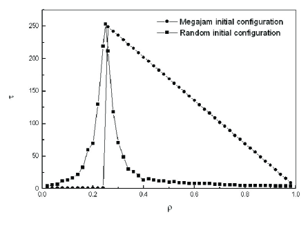
Figure 1: The relaxation time $\tau$ as a function of the vehicle density $\rho$ in the deterministic NS model with different initial configuration for the case of $v_{\max}=3$, $L=1000$.

III NUMERICAL RESULTS

First, we investigate the influences of the initial configuration on the relaxation time $\tau$ of energy dissipation $e(t)$ in the deterministic NS model. In the deterministic case, the stochastic braking is not considered, i.e. $p=0$. Figure 1 shows the relaxation time $\tau$ as a function of the vehicle density $\rho$ with megajam and random initial configuration in the case of $v_{\max}=3,L=1000$. As shown in Fig. 1, there is a critical slowing down; and the relaxation to the steady state becomes quite slow close to the critical density $\rho_{c}=1/(1+v_{\max})$. The relaxation time $\tau$ diverges at the critical density $\rho_{c}$ in the model with random initial configuration, which are consistent with a second-order phase transition. In the case of megajam initial configuration, however, the relaxation time $\tau$ is invalid below the critical density $\rho_{c}$ for there is no energy dissipation occurs at any time. Above the critical density, $\tau$ decreases linearly with increasing the vehicle density. As reported in Refs.[15 ], above the critical density $\rho_{c},$ energy dissipation rate $E_{d}$ occurs abruptly and reaches the maximum value in the system with megajam initial condition, which is different from that with random initial configuration. The phase transition is not continuous. Thus, we argue that the dynamical transition from free-flow traffic to jammed state in the system with megajam initial condition can be viewed as first-order phase transition. In the jammed phase, the relaxation to the steady state in the system with megajam initial condition is slower than that with random initial configuration, as shown in Fig. 1.

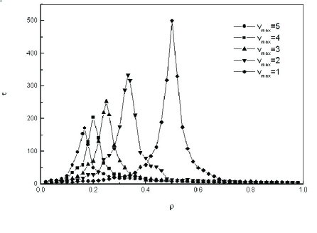
Figure 2: The relaxation time $\tau$ as a function of the vehicle density $\rho$ for various values of the speed limit $v_{\max}$ in the deterministic NS model with random initial configuration for the case of $L=1000$.

Figure 2 shows the relaxation time $\tau$ as a function of the vehicle density $\rho$ with different values of the speed limit $v_{\max}$ in the case of random initial configuration. From figure 2, we see that the maximal value of relaxation time $\tau_{m}$ occurs at the critical density $\rho_{c}.$ And the time $\tau_{m}$ decreases with the increase of speed limit $v_{\max}.$ The relaxation time $\tau_{m}$ is given as

$$\tau_{m}=\frac{L}{v_{\max}+1},\qquad\qquad(3)$$

which is compatible with the results obtained with another order parameter14 . Figure 3 shows the relaxation time $\tau_{m}$ as a function of the system size $L$ with different values of the speed limit $v_{\max}.$ As shown in figure 3, symbol data are obtained from computer simulations, and solid lines correspond to analytic results of the formula (3).

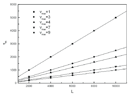
Figure 3: The relaxation time $\tau_{m}$ as a function of the lattice size $L$ for various values of the speed limit $v_{\max}$ in the deterministic NS model with random initial configuration. Symbol data are obtained from computer simulations, and solid line corresponds to analytic results of the formula (3).

Figure 4 shows the relaxation time $\tau$ as a function of the vehicle density $\rho$ with different values of the speed limit $v_{\max}$ in the case of megajam initial configuration. From figure 4, we see that the relaxation time $\tau$ decreases linearly with the increase of the vehicle density over the critical density $\rho_{c}$. The relaxation time $\tau$ can be written as

$$\tau=\frac{L}{v_{\max}}(1-\rho).\qquad\qquad(4)$$

In figure 4, symbol data are obtained from computer simulations, and solid lines correspond to analytic results of the formula (4). Compared with the theoretical results and simulation data, excellent agreement can be obtained.

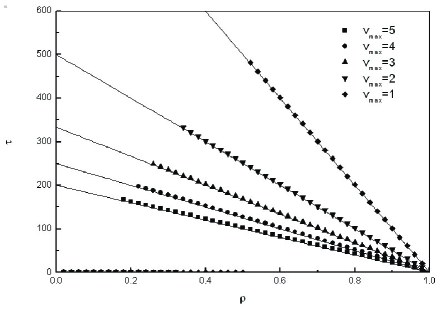
Figure 4: The relaxation time $\tau$ as a function of the vehicle density $\rho$ for various values of the speed limit $v_{\max}$ in the deterministic NS model with megajam initial configuration for the case of $L=1000$.. Symbol data are obtained from computer simulations, and solid line corresponds to analytic results of the formula (4).

In the deterministic case, i.e. $p=0$, the order parameter $E_{d}$ is zero when $\rho\leq\rho_{c}$ and $E_{d}>0$ in the density interval $1>\rho>\rho_{c}.$ However, in the case of $p\neq 0$, the parameter $E_{d}$ is not zero anymore. The phase transition observed in the deterministic case is destroyed by the stochastic braking probability $p$. The probability $p$ is the conjugated parameter of the order parameter of NS model. In order to analyze the relationship between the probability $p,$ energy dissipation rate $E_{d}$ and phase behavior, we define the associated susceptibility

$$\chi_{p}=\left.\frac{\partial E_{d}}{\partial p}\right|_{p=0}.\qquad\qquad(5)$$

Figure 5: The susceptibility $\chi_{p}$ as a function of the vehicle density $\rho$ in NS model with random initial configuration for various values of the speed limit $v_{\max},$ for the case of $L=10000$ and $p=0.01.$

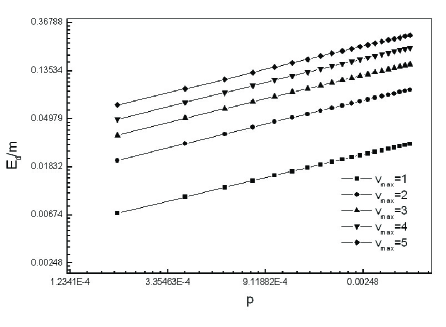
Figure 6: The log-log plot of energy dissipation rate $E_{d}$ (scaled by $m$ ) at the critical density $\rho_{c}$ as a function of the stochastic braking probability $p$ in NS model with random initial configuration for the case of $L=10000$, for various values of the speed limit $v_{\max}$.

Figure 5 exhibits the relation of $\chi_{p}$ to the vehicle density $\rho$ with various values of the speed limit and random initial condition in the case of $p=0.01,L=10000$. As shown in figure 5, the susceptibility $\chi_{p}$ first increases with the density $\rho$, then it decreases with $\rho$ above the critical density $\rho_{c}$ where a maximum value is reached. At high density region, the susceptibility $\chi_{p}$ is negative, i.e. energy dissipation rate $E_{d}$ decreases with increasing the probability $p$. When $\rho>0.8,$ the curves converges into one curve and $v_{\max}$ has no influence on $\chi_{p}$. The peak’s values increase with the increase of the speed limit $v_{\max}.$ The peak of $\chi_{p}$ tends to diverge at the critical density $\rho_{c}$ in the case of $p\rightarrow 0$. The divergence of $\chi_{p}$ is relevant to the traffic phase transition.

From figure 5, we can observe that $\chi_{p}$ $\propto v_{\max}$ when $\rho\rightarrow 0$. At the critical density $\rho_{c},$ for $p\rightarrow 0,$ we find that the order parameter $E_{d}{}$ follows a power-law behavior of the form

$$E_{d}{}\propto p^{\gamma}.\qquad\qquad(6)$$

Figure 7: Time evolutions of energy dissipation $e(t)$ (scaled by $m$ ) starting from the random and megajam initial configuration for the case of $v_{\max}=3$, $p=0.005$, $\rho=0.3$ and $L=1000$.

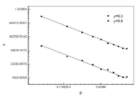
Figure 8: The relaxation time $\tau$ as a function of stochastic braking probability $p$ near the limit $p\rightarrow 0$ for several fixed density in NS model with megajam initial configuration for the case of $v_{\max}=3$ and $L=1000$. Lines are guides for the eyes.

Figure 6 shows that the critical exponent $\gamma\approx 0.483\pm 0.005$ and the speed limit has no influences on $\gamma.$ In the NS model with megajam initial configuration, the behavior of $\chi_{p}$ is similar with that with random initial condition. The dynamic exponent $\gamma$ remains unchanged when varying the initial configuration. However, the initial condition has effects on the relaxation time $\tau$ near the limit $p\rightarrow 0$. Figure 7 exhibits time evolutions of $e(t)$ starting from the megajam and random initial configuration in the case of $v_{\max}=3,p=0.005,L=1000$ and $\rho=0.3.$ As shown in figure 7, the relaxation to steady state in the system with megajam initial condition is slower than that with random configuration, even if the values of $e(t)$ at the steady state are unique. Figure 8 exhibits the relation of relaxation time $\tau$ to the stochastic braking probability $p$ near the limit $p\rightarrow 0$ with various values of vehicle density. From figure 8, we see that

$$\tau\propto p^{-\delta},\qquad\qquad(7)$$

and the dynamic exponent $\delta\approx 1.04\pm 0.02.$

Figure 9: The relaxation time $\tau$ as a function of the system size $L$ with megajam initial configuration for the case of $v_{\max}=3$,$\rho=0.3$ and $p=0.005$.

Figure 9 shows the relaxation time $\tau$ as a function of the system size $L$ with megajam initial configuration in the case of $v_{\max}=3$,$\rho=0.3$ and $p=0.005$. As shown in figure 9, the relaxation time $\tau$ has a scaling form

$$\tau\propto L^{\nu},\qquad\qquad(8)$$

and the exponent $\nu\approx 1,$ which is compatible with the results presented in Refs.[17,18].

IV SUMMARY

In this paper, we investigate traffic phase transition behavior in the NS model considering different initial configurations. Different initial condition gives rise to distinct phase transition. We argue that the phase transition in the system with megajam and random configuration is first- and second-order phase transition, respectively. Using the order parameter $E_{d}$, we numerically studied the relaxation time $\tau$ and susceptibility $\chi_{p}.$ The two quantities diverge at the critical density $\rho_{c}.$ We analyzed the relaxation time $\tau_{m}$ and $\tau$ theoretically. Theoretical analyses give an excellent agreement with numerical results. Near the limit $p\rightarrow 0$, the parameter $E_{d}$ and relaxation time $\tau$ follow a power-law behavior. The dynamic exponent $\gamma\approx 0.483\pm 0.005$, $\delta\approx 1.04\pm 0.02$ and $\nu\approx 1.$

When $p\nrightarrow 0$, the phase transition behavior becomes more complicated. We will make further investigation using the order parameter $E_{d}$. The associated dynamic exponents and scaling laws will be presented elsewhere.

References

- (1) D. Chowdhury, L. Santen, and A. Schadschneider, Phys.Rep. 329, 199 (2000), and references therein.
- (2) D. Helbing, Rev. Mod. Phys. 73, 1067 (2001).
- (3) T. Nagatani, Rep. Prog. Phys. 65, 1331 (2002).
- (4) S. Maerivoet and B. De Moor, Phys. Rep. 419, 1 (2005).
- (5) K. Nagel and M. Schreckenberg, J. Phys. I 2, 2221 (1992).
- (6) L. C. Q. Vilar and A. M. C. de Souza, Physica A 211, 84 (1994).
- (7) G Csanyi and J Kertesz, J. Phys. A: Math. Gen. 28, L427 (1995).
- (8) M. Sasvari and J. Kertesz, Phys. Rev. E 56, 4104 (1997).
- (9) B. Eisenblatter, L. Santen, A. Schadschneider and M. Schreckenberg, Phys. Rev. E 57, 1309 (1998).
- (10) L. Neubert, H.Y. Lee and M. Schreckenberg, J. Phys. A 32, 6517 (1999).
- (11) L. Roters, S. L¨1beck, and K. D. Usadel, Phys. Rev. E 59, 2672 (1999).
- (12) D. Chowdhury, J. Kertesz, K. Nagel, L. Santen and A. Schadschneider, Phys. Rev. E 61, 3270 (2000).
- (13) N. Boccara and H. Fuks, J. Phys. A: Math. Gen. 33, 3407 (2000).
- (14) A. M. C. Souza and L. C. Q. Vilar, Phys. Rev. E 80, 021105 (2009).
- (15) W. Zhang, W. Zhang, and X.-Q. Yang, Physica A 387, 4657 (2008).
- (16) D. Helbing, Phys. Rev. E 55, 3735 (1997).
- (17) K.Nagel and H. J. Herrmann, Physica A 199, 245 (1993).
- (18) N. Moussa, Phys. Rev. E 77, 026124 (2005).