Gauge invariant Ansatz for a special three-gluon vertex

Abstract

We construct a general Ansatz for the three-particle vertex describing the interaction of one background and two quantum gluons, by simultaneously solving the Ward and Slavnov-Taylor identities it satisfies. This vertex is known to be essential for the gauge-invariant truncation of the Schwinger-Dyson equations of QCD, based on the pinch technique and the background field method. A key step in this construction is the formal derivation of a set of crucial constraints (shown to be valid to all orders), relating the various form factors of the ghost Green’s functions appearing in the aforementioned Slavnov-Taylor identity. When inserted into the Schwinger-Dyson equation for the gluon propagator, this vertex gives rise to a number of highly non-trivial cancellations, which are absolutely indispensable for the self-consistency of the entire approach.

I Introduction

In recent years, a significant part of the ongoing activity dedicated to the study the non-perturbative sector of Yang-Mills theories, and especially of QCD, has focused on the infrared behavior of individual Green’s functions. The information obtained by a variety of large-volume lattice simulations has been of singular importance for advancing in this direction, and has stimulated an in-depth re-examination of various aspects of the underlying QCD dynamics. In particular, these lattice results clearly indicate that the gluon propagator and the ghost dressing function of pure Yang-Mills theories, computed in the conventional Landau gauge, are infrared finite, both in $SU(2)$ Cucchieri:2007md ; Cucchieri:2007rg ; Cucchieri:2009zt ; Cucchieri:2011ga ; Cucchieri:2011um and in $SU(3)$ Bogolubsky:2007ud ; Bowman:2007du ; Bogolubsky:2009dc ; Oliveira:2009eh .

Evidently, reproducing these (and related) lattice results using continuous approaches represents a highly non-trivial challenge. In this effort, the Schwinger-Dyson equations (SDEs) constitute an obvious (albeit technically cumbersome) starting point. As has been argued in a series of recent articles Aguilar:2006gr ; Binosi:2007pi ; Binosi:2008qk , the modified set of SDEs obtained within the general formalism based on the Pinch Technique (PT) Cornwall:1981zr ; Cornwall:1989gv ; Binosi:2002ft ; Binosi:2003rr ; Binosi:2009qm and the Background Field Method (BFM) Abbott:1980hw , is particularly well-suited for attempting this difficult task (for alternative approaches see, e.g., Alkofer:2000wg ; Fischer:2006ub ; Dudal:2008sp ; Boucaud:2008ji ; Braun:2007bx ; Szczepaniak:2010fe ; RodriguezQuintero:2010ss ; RodriguezQuintero:2010yq ).

One of the key ingredients of the PT-BFM approach, in general, is (see Fig. 1) the three-gluon vertex describing the interaction between one background ($B$) and two quantum ($Q$) gluons (“$BQQ$ vertex”, for short). This vertex appears naturally in the modified SDE governing the gluon self-energy, and is instrumental for its gauge-invariant truncation. In particular, and contrary to what happens in the conventional formulation, the “one-loop dressed” subset of (only gluonic!) diagrams (see Fig. 2), corresponding to the first step in the aforementioned SDE truncation, furnishes an exactly transverse gluon self-energy. In addition, the way the gluon acquires a dynamically generated (momentum-dependent) mass Cornwall:1981zr , which, in turn, accounts for the infrared finiteness of the aforementioned Green’s functions, is determined by a subtle interplay of all the ingredients entering into the corresponding SDE. In this context the non-perturbative form of the $BQQ$ vertex is essential for obtaining infrared finite results out of the SDEs considered, without violating any of the underlying field-theoretic principles Aguilar:2009ke .

A major difficulty that is typical in the SDE studies (and not only in the case of the $BQQ$ vertex considered here) is precisely the form that one must use for the various fully-dressed vertices entering into the problem. To be sure, the non-perturbative behavior of each such vertex (including the $BQQ$ vertex) is determined by its own SDE equation, which contains the various multiparticle kernels appearing in the “skeleton expansion” (see Fig. 3). However, for practical purposes, one is forced to resort to an Ansatz for this vertex, obtained through the so-called “gauge-technique” Salam:1963sa ; Salam:1964zk ; Delbourgo:1977jc ; Delbourgo:1977hq .

The idea behind the gauge-technique is fairly simple, even though its precise implementation may be rather complicated. Specifically, one constructs an expression for the unknown vertex out of the ingredients appearing in the Ward identity (WI) and/or the Slavnov-Taylor identity (STI) it satisfies. These ingredients must be put together in a way such that the resulting expression satisfies the WI and/or the STI automatically. Evidently, this technique becomes more difficult to implement as the Lorentz and color structure of the vertex under construction increases, and the structure of the STIs that it satisfies gets more involved. In addition, it is clear that this method can only determine the “longitudinal” part of any vertex, leaving its “transverse” (i.e., automatically conserved) part completely unspecified. Failing to provide the correct transverse part leads to the mishandling of overlapping divergences, which, in turn, compromises the multiplicative renormalizability of the resulting SDE. The usual remedy employed in the literature is to account approximately for the missing pieces by modifying appropriately (but“by hand”) the SDE in question.

In this article we will cary out in detail the gauge-technique construction for the $BQQ$ vertex mentioned above. This is a particularly involved task, and deviates appreciably from the corresponding construction of the conventional three-gluon vertex (the “$QQQ$ vertex” in this notation) Ball:1980ax , mainly for the following reasons.

• Unlike the $QQQ$ vertex, which displays Bose symmetry with respect to the interchange of any one of its three legs, the $BQQ$ vertex is Bose symmetric only under the interchange of the two quantum legs. As a result, the constraints imposed by Bose symmetry on the various form-factors comprising the two vertices are different.

• Whereas the $QQQ$ vertex satisfies the same STI when contracted from any direction, the $BQQ$ vertex satisfies an Abelian (ghost-free) WI when contracted from the side of the background gluon, and an STI when contracted from the side of either one of the quantum gluons [see Eq. (9)].

• The number of Green’s functions and composite (BRST-induced) operators entering into the STI satisfied by the $BQQ$ is practically duplicated compared to the $QQQ$ case. Indeed, while the the STI maintains its basic characteristic form, any Green’s function that appears in it and has an incoming gluon (i.e., gluon self-energy or the “gluon-ghost” kernel) appears in two versions: in the first, the incoming gluon is a quantum gluon, in the second, it is a background one [the latter quantities are denoted by “tildes” on the rhs of Eq. (9)].

As is well-known from the case of the conventional vertex Ball:1980ax , the gauge-technique construction boils down finally to the solution of a system of various equations, whose unknowns are the form factors (of the longitudinal part) of the vertex under construction. The solution of this system allows to express these form factors in terms of the various quantities appearing on the rhs of the STI: gluon propagator(s), ghost dressing function, and a subset of the form factors of the “gluon-ghost” kernel(s). However, solving the resulting system is conceptually subtle, because the additional constrains imposed by Bose-symmetry reduces the number of unknowns, and one is left with more equations than unknowns. Thus, in order to find non-trivial solutions, a set of additional identities must be imposed, which relates the ingredients appearing on the rhs of the STI; in particular, the ghost dressing function is related to some of the form-factors of the “gluon-ghost” kernels [see Eqs. (35) and (36)]. This reduces the number of available equations, because some of them are identically satisfied, precisely by virtue of these additional identities. These identities can be established by inspection, i.e., as a necessary condition for having non-trivial solutions for the system. However, given that they constitute, at the same time, non-trivial relations between well-defined field-theoretic quantities (those appearing on the rhs of the STI), their validity must hold regardless of the need to solve the given system of equations. In the work of Ball:1980ax the aforementioned set of crucial auxiliary identities has been established as a necessary condition for solving the system, and their validity has been indeed confirmed at the one-loop perturbative level, through an explicit calculation (the complete one-loop off-shell form factors, in an arbitrary covariant gauge $\xi$ and space-time dimension, have been calculated in Davydychev:1996pb ).

In the case of the $BQQ$ vertex we consider, and given the aforementioned duplication of the quantities entering into the STI, the solution of the system requires the validity of two types of such auxiliary identities: one of them coincides with that found in Ball:1980ax , while the other is completely new, and reported here for the first time. It turns out that the validity of both identities can be demonstrated to all-orders (and non-perturbatively); indeed, they are a direct consequence of a STI and a WI that the two ghost sectors (the “conventional” one and the “tilded” one, respectively) satisfy. To the best of our knowledge this is a novel result.

The article is organized as follows. In Section II we present some basic facts about the $BQQ$ vertex. We pay particular attention to the WI and STI this vertex satisfies, and explain in detail the definition and field-theoretic origin of the various quantities entering in them. In Section III we resort to the Batalin-Vilkovisky formalism, in order to derive the auxiliary STI and WI satisfied by the two types of ghost-induced Green’s functions appearing in the central STI (satisfied by $BQQ$). These two auxiliary equations are valid to all orders, and give rise to the set of constraints needed for the solution of the system in the next section. Section IV contains the main result of this article. Specifically, the system of equations involving the form factors of the longitudinal part of the vertex is presented, and its solution is reported, after using the additional constraints derived in the previous section. In Section V we give a detailed account of the most important theoretical consequences that the precise form of the vertex has for the SDE of the gluon propagator (in the Landau gauge). Finally, in Section VI we present our conclusions.

II The $BQQ$ vertex and its basic properties

The $BQQ$ vertex constitutes without any doubt one of the most fundamental ingredients of the pinch technique, making its appearance already at the basic level of the one-loop construction. Specifically, defining the tree-level conventional three-gluon vertex through the expression (all momenta entering)

$$i\Gamma^{(0)}_{A^{a}_{\alpha}A^{b}_{\mu}A^{c}_{\nu}}(q,r,p) = gf^{abc}\Gamma^{(0)}_{\alpha\mu\nu}(q,r,p)$$

$$\Gamma^{(0)}_{\alpha\mu\nu}(q,r,p) = g_{\mu\nu}(r-p)_{\alpha}+g_{\alpha\nu}(p-q)_{\mu}+g_{\alpha\mu}(q-r)_{\nu},$$ (1)

the diagrammatic rearrangements giving rise to the PT Green’s functions (propagators and vertices) stem exclusively from the characteristic decomposition Cornwall:1981zr ; Cornwall:1989gv ; Pilaftsis:1996fh

$$\Gamma^{(0)}_{\alpha\mu\nu}(q,r,p) = \widetilde{\Gamma}^{(0)}_{\alpha\mu\nu}(q,r,p)+(1/\xi)\Gamma^{{\rm P}}_{\alpha\mu\nu}(q,r,p),$$

$$\widetilde{\Gamma}^{(0)}_{\alpha\mu\nu}(q,r,p) = g_{\mu\nu}(r-p)_{\alpha}+g_{\alpha\nu}(p-q+r/\xi)_{\mu}+g_{\alpha\mu}(q-r-p/\xi)_{\nu},$$

$$\Gamma^{{\rm P}}_{\alpha\mu\nu}(q,r,p) = g_{\alpha\mu}p_{\nu}-g_{\alpha\nu}r_{\mu}.$$ (2)

In the equations above, $\xi$ represents the gauge-fixing parameter that appears also in the definition of the (full) gluon propagator $\Delta^{ab}_{\mu\nu}(q)=\delta^{ab}\Delta_{\mu\nu}(q)$, with

$$i\Delta_{\mu\nu}(q)=-i\left[P_{\mu\nu}(q)\Delta(q^{2})+\xi\frac{q_{\mu}q_{\nu}}{q^{4}}\right];\qquad\Delta^{-1}_{\mu\nu}(q)=i\left[P_{\mu\nu}(q)\Delta^{-1}(q^{2})+(1/\xi)q_{\mu}q_{\nu}\right]$$ (3)

and $P_{\mu\nu}(q)=g_{\mu\nu}-q_{\mu}q_{\nu}/q^{2}$ the dimensionless transverse projector; finally, the scalar cofactor $\Delta(q^{2})$ is finally related to the all-order gluon self-energy $\Pi_{\mu\nu}(q)=P_{\mu\nu}(q)\Pi(q^{2})$ through

$$\Delta^{-1}({q^{2}})=q^{2}+i\Pi(q^{2})=q^{2}J(q^{2}).$$ (4)

Notice that the PT makes no ab initio reference to a background gluon; at the level of the Yang-Mills Lagrangian there is only one gauge field, $A$, which is quantized in the usual way, by means of a linear gauge-fixing function of the $R_{\xi}$ type ${\cal F}^{a}=\partial^{\mu}A^{a}_{\mu}$. However, the decomposition (2) assigns right from the start a special role to the leg carrying the momentum $q$, that is to be eventually identified with the background leg. Thus, unlike $\Gamma^{(0)}$, which is Bose-symmetric with respect to all its three legs, the vertex $\widetilde{\Gamma}^{(0)}$ is in fact Bose-symmetric only with respect to the (quantum) $\mu$ and $\nu$ legs. In addition, it satisfies the simple Ward identity

$$iq^{\alpha}\widetilde{\Gamma}^{(0)}_{\alpha\mu\nu}(q,r,p)=\Delta^{-1}_{0\,\mu\nu}(p)-\Delta^{-1}_{0\,\mu\nu}(r),$$ (5)

where the sub-index “0” on the rhs indicates the tree-level version of the inverse propagator (3). In higher orders, the $BQQ$ vertex is constructed through the systematic triggering of internal STIs in the diagrams of the conventional (higher order) three-gluon vertex Binosi:2002ft ; Binosi:2003rr .

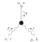
Figure 1: The $BQQ$ three-gluon vertex. The background leg is indicated by the gray circle.

On the other hand, when quantizing the theory within the BFM, the notion of a $BQQ$ vertex $\Gamma_{\widehat{A}AA}$ arises naturally as a consequence of the splitting of the classical gauge field into a background and a quantum part, $A\to A+\widehat{A}$, and the choice of a special gauge fixing function ${\cal F}^{a}=\partial^{\mu}A^{a}_{\mu}+gf^{abc}\widehat{A}^{\mu}_{b}A_{\mu}^{c}$, which is linear in the quantum field $A$, and preserves gauge invariance with respect to the background field $\widehat{A}$. The latter induces to the tree-level $BQQ$ vertex an additional dependence on the gauge-fixing parameter $\xi_{Q}$, and one has (see Fig. 1)

$$i\Gamma_{\widehat{A}^{a}_{\alpha}A^{b}_{\mu}A^{c}_{\nu}}(q,r,p)=gf^{abc}\widetilde{\Gamma}_{\alpha\mu\nu}(q,r,p);$$ (6)

the tree-level value of the vertex in Eq. (6), namely $\widetilde{\Gamma}^{(0)}$, coincides with the PT expression of Eq. (2), after the replacement $\xi\to\xi_{Q}$. This equality between the PT and BFM construction appears to be rather general; for the usual two- and three-point functions (such as the gluon propagator, quark-gluon vertex, and three-gluon vertex) it has been shown to hold both perturbatively (to all orders) Binosi:2002ft ; Binosi:2003rr , and non-perturbatively (at the SDE level) Binosi:2007pi ; Binosi:2008qk .

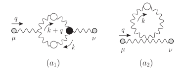
Figure 2: The one-loop dressed gluon contribution to the PT-BFM gluon self-energy. Notice that, contrary to what happens within the conventional formalism these two diagrams constitute a transverse subset of the full SDE.

As mentioned in the Introduction, the $BQQ$ vertex $\widetilde{\Gamma}$ enters into the SDE satisfied by the PT-BFM gluon propagator. Specifically, considering the (gauge-invariant) subset of fully dressed diagrams of Fig. 2, one finds

$$(a_{1})_{\mu\nu} = \frac{1}{2}\,g^{2}C_{A}\int_{k}\!\widetilde{\Gamma}^{(0)}_{\mu\alpha\beta}\Delta^{\alpha\rho}(k)\Delta^{\beta\sigma}(k+q)\widetilde{\Gamma}_{\nu\rho\sigma}$$

$$(a_{2})_{\mu\nu} = g^{2}C_{A}\left[g_{\mu\nu}\int_{k}\!\Delta^{\rho}_{\rho}+\left(1/\xi-1\right)\int_{k}\!\Delta_{\mu\nu}\right],$$ (7)

with the $d$-dimensional integral measure (in dimensional regularization) defined as

$$\int_{k}\equiv\frac{\mu^{\epsilon}}{(2\pi)^{d}}\!\int\!\mathrm{d}^{d}k.$$ (8)

Evidently, non-perturbative information on the vertex $\widetilde{\Gamma}$ is essential for making further progress with these equations. In principle, the complete structure of $\widetilde{\mathrm{I}\!\Gamma}$ is determined from its own SDE; however, this equation is practically intractable, given that it involves several unknown one-particle reducible kernels, associated with its skeleton expansion shown in Fig. 3. Given this serious limitation, one usually is forced to approximate the vertex by employing a suitable Ansatz. In general, such an Ansatz is obtained by resorting to the aforementioned gauge technique Salam:1963sa ; Salam:1964zk ; Delbourgo:1977jc ; Delbourgo:1977hq . Even though the actual construction will be carried out in Section IV, it is worthwhile to briefly review the basic philosophy behind this technique.

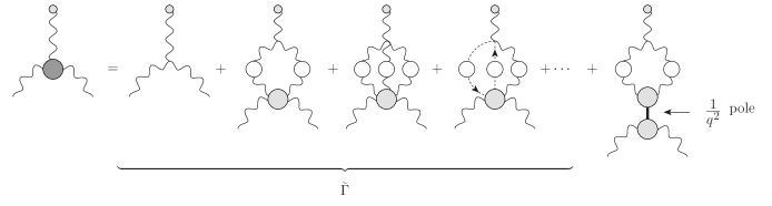
Figure 3: The SDE equation for the $BQQ$ vertex $\widetilde{\Gamma}$. The first diagrams correspond to the standard skeleton expansion in terms of one-particle irreducible multi-leg kernels (grey blobs). The last term, representing a non-perturbative bound-state pole, appears only when the Schwinger mechanism Schwinger:1962tn ; Schwinger:1962tp is triggered Jackiw:1973tr ; Cornwall:1973ts ; Eichten:1974et .

The main idea is easier captured in the Abelian context where it was first applied. Roughly speaking, one constructs an expression for the unknown vertex out of the ingredients appearing in the WI it satisfies. These ingredients must be put together in a way such that the resulting expression satisfies the WI automatically. The most typical example of such a construction is found in the case of the three-particle vertex of scalar QED, describing the interaction of a photon with a pair of charged scalars. This vertex, to be denoted by $\Gamma_{\mu}$, satisfies the abelian all-order WI

$$q^{\mu}\Gamma_{\mu}={\mathcal{D}}^{-1}(k+q)-{\mathcal{D}}^{-1}(k)\,,$$ (9)

where ${\mathcal{D}}(k)$ is the fully-dressed propagator of the scalar field. Thus, in this case, the gauge-technique Ansatz for $\Gamma_{\mu}$, obtained by Ball and Chiu Ball:1980ay , after “solving” the above WI, under the additional requirement of not introducing kinematic singularities, is

$$\Gamma_{\mu}=\frac{(2k+q)_{\mu}}{(k+q)^{2}-k^{2}}\left[{\mathcal{D}}^{-1}(k+q)-{\mathcal{D}}^{-1}(k)\right],$$ (10)

which clearly satisfies Eq. (9).

Of course, this construction is significantly more complicated for the $BQQ$ vertex $\widetilde{\mathrm{I}\!\Gamma}$, since the identities imposed by the BRST symmetry are far more complex than the simple Abelian WI of Eq. (9); indeed, in order to cast these upcoming identities into a more compact form, it is convenient to consider, instead of $\widetilde{\Gamma}$, the minimally modified vertex $\widetilde{\mathrm{I}\!\Gamma}$, defined as

$$\widetilde{\mathrm{I}\!\Gamma}_{\alpha\mu\nu}(q,r,p)=\widetilde{\Gamma}_{\alpha\mu\nu}(q,r,p)+(1/\xi_{Q})\Gamma^{\rm{P}}_{\alpha\mu\nu}(q,r,p).$$ (11)

Evidently, $\widetilde{\mathrm{I}\!\Gamma}_{\alpha\mu\nu}(q,r,p)$ and $\widetilde{\Gamma}_{\alpha\mu\nu}(q,r,p)$ differ only at tree level; specifically, using Eq. (2), we see immediately that

$$\widetilde{\mathrm{I}\!\Gamma}_{\alpha\mu\nu}^{(0)}(q,r,p)=\Gamma^{(0)}_{\alpha\mu\nu}(q,r,p).$$ (12)

Incidentally, notice that $\widetilde{\mathrm{I}\!\Gamma}_{\alpha\mu\nu}(q,r,p)$ coincides with the vertex appearing in diagram $(a_{1})$ of the SDE (7), when projected to the Landau gauge Aguilar:2008xm , see also Section V.

Then, the vertex $\widetilde{\mathrm{I}\!\Gamma}$ satisfies a (ghost-free) WI when contracted with the momentum $q_{\alpha}$ of the background gluon, whereas it satisfies a STI when contracted with the momentum of the quantum gluons ($r_{\mu}$ or $p_{\nu}$). They read

$$q^{\alpha}\widetilde{\mathrm{I}\!\Gamma}_{\alpha\mu\nu}(q,r,p) = p^{2}J(p^{2})P_{\mu\nu}(p)-r^{2}J(r^{2})P_{\mu\nu}(r)$$

$$r^{\mu}\widetilde{\mathrm{I}\!\Gamma}_{\alpha\mu\nu}(q,r,p) = F(r^{2})\left[q^{2}\widetilde{J}(q^{2})P_{\alpha}^{\mu}(q)H_{\mu\nu}(q,r,p)-p^{2}J(p^{2})P_{\nu}^{\mu}(p)\widetilde{H}_{\mu\alpha}(p,r,q)\right]$$

$$p^{\nu}\widetilde{\mathrm{I}\!\Gamma}_{\alpha\mu\nu}(q,r,p) = F(p^{2})\left[r^{2}J(r^{2})P_{\mu}^{\nu}(r)\widetilde{H}_{\nu\alpha}(r,p,q)-q^{2}\widetilde{J}(q^{2})P_{\alpha}^{\nu}(q)H_{\nu\mu}(q,p,r)\right],$$ (13)

where $F(q^{2})$ represents the ghost dressing function, related to the ghost propagator $D^{ab}(q^{2})=\delta^{ab}D(q^{2})$ through

$$iD(q^{2})=i\frac{F(q^{2})}{q^{2}},$$ (14)

and the function $\widetilde{J}$ is related to the conventional one defined in (3) through the so-called “background quantum identity” Grassi:1999tp ; Binosi:2002ez

$$\widetilde{J}(q^{2})=\left[1+G(q^{2})\right]J(q^{2}).$$ (15)

Finally, the function $G$ appearing above is the metric form factor in the Lorentz decomposition of the auxiliary function $\Lambda$, defined as

$$\Lambda_{\mu\nu}(q) = -ig^{2}C_{A}\int_{k}\!\Delta_{\mu}^{\sigma}(k)D(q-k)H_{\nu\sigma}(-q,q-k,k)$$ (16)

$$= g_{\mu\nu}G(q^{2})+\frac{q_{\mu}q_{\nu}}{q^{2}}L(q^{2}),$$

with $C_{A}$ the Casimir eigenvalue of the adjoint representation [$C_{A}=N$ for $SU(N)$]. This function, together with the definitions and conventions for the auxiliary functions $H$ and $\widetilde{H}$, which will be studied in great detail in the next section, is shown in Fig. 4. Thus, requiring the vertex Ansatz to satisfy the STIs above implies that in its expression certain combinations of the ghost auxiliary functions $G$, $H$ and $\widetilde{H}$ will also appear.

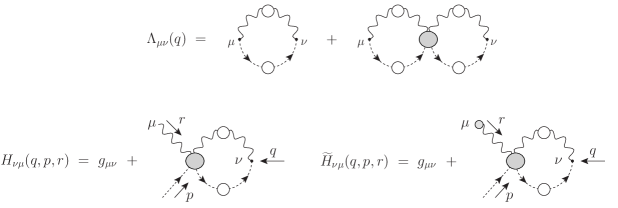
Figure 4: Definitions and conventions of the auxiliary functions $\Lambda$, $H$ and $\widetilde{H}$. The color and coupling dependence for the combination shown, $c^{a}(q)A_{\mu}^{b}(r)A_{\nu}^{*c}(p)$, is $gf^{acb}$. White blobs represent connected Green’s functions, while gray blobs denote one-particle irreducible (with respect to vertical cuts) kernels.

III Identities of the ghost sector

In view of the prominent role played by the ghost auxiliary functions $H$ and $\widetilde{H}$ in the ensuing analysis, in this section we shall study them, as well as the identities they satisfy. The framework that allows us to do this is the one developed long ago by Batalin and Vilkovisky Batalin:1977pb ; Batalin:1981jr , that we very briefly review below.

In the Batalin-Vilkovisky formulation of Yang-Mills theories, one starts by introducing certain sources (called anti-fields and represented with a * super-index) and couples them to the corresponding field through the term $\Phi^{*}s\,\Phi$ where $s$ is the BRST operator. Since these anti-fields will describe the renormalization of composite operators, they might be introduced only for those fields that transform non-linearly under the BRST operator; in the case of the $SU(N)$ Yang-Mills theories that we consider, this means for the gluon and ghost field only, since

$$sA^{a}_{\mu}=({\cal D}^{\mu}c)^{a};\qquad sc^{a}=-\frac{1}{2}gf^{abc}c^{b}c^{c}$$ (17)

where ${\cal D}$ is the usual covariant derivative with $({\cal D}_{\mu}\Phi)^{a}=\partial_{\mu}\Phi^{a}+gf^{abc}A^{b}_{\mu}\Phi^{c}$.

In much the same way, the quantization of the theory in a background field type of gauge requires, in addition to the aforementioned anti-fields, the introduction of new sources which couple to the BRST variation of the background fields Grassi:1999tp . These sources are sufficient for implementing the full set of symmetries at the quantum level, and, in the case of $SU(N)$ Yang-Mills theories, after choosing a linear gauge fixing function (e.g., $R_{\xi}$ or BFM type of gauges), we are lead to the master equation

$$\int{\rm d}^{4}x\left[\frac{\delta\Gamma}{\delta A^{*\mu}_{a}}\frac{\delta\Gamma}{\delta A^{a}_{\mu}}+\frac{\delta\Gamma}{\delta c^{*a}}\frac{\delta\Gamma}{\delta c^{a}}+\Omega^{\mu}_{a}\left(\frac{\delta\Gamma}{\delta\widehat{A}^{a}_{\mu}}-\frac{\delta\Gamma}{\delta A^{a}_{\mu}}\right)\right]=0.$$ (18)

In the formula above, $\Gamma$ is the (reduced) effective action, $A^{*}$ and $c^{*}$ the gluon and ghost anti-fields, $\widehat{A}$ is the gluon background field, and $\Omega$ the corresponding background source.

For the study of the algebraic structure $H$ and $\widetilde{H}$, we will need two additional equations. The first one is the Faddeev-Popov equation, which controls the result of the contraction of an anti-field leg with the corresponding momentum. In position space, it reads

$$\frac{\delta\Gamma}{\delta\bar{c}^{a}}+\left(\widehat{\cal D}^{\mu}\frac{\delta\Gamma}{\delta A^{*}_{\mu}}\right)^{a}-\left({\cal D}^{\mu}\Omega_{\mu}\right)^{a}-gf^{amn}\widehat{A}^{m}_{\mu}\Omega^{\mu}_{n}=0,$$ (19)

where $\widehat{\cal D}$ is the background covariant derivative (obtained from the usual one by replacing the gluon field $A$ with the background field $\widehat{A}$). Notice that Eqs. (18) and (19) above are given for the BFM gauge; to get the analogous expressions for the conventional $R_{\xi}$ gauges, one needs to set the background field and source $\widehat{A}$ and $\Omega$ to zero, and $\Gamma\to\left.\Gamma\right|_{\widehat{A},\Omega=0}$.

The second equation furnishes the WI functional ${\cal W}$, which encodes the residual background gauge invariance; it reads

$${\cal W}_{\vartheta}[\Gamma]=\int\!{\rm d}^{4}x\!\sum_{\varphi=\Phi,\Phi^{*}}\!\left(\delta_{\vartheta}\varphi\right)\frac{\delta\Gamma}{\delta\varphi}=0,$$ (20)

where $\vartheta^{a}$ (which, in this case, plays the role of the ghost field) is the local infinitesimal parameter associated with the $SU(N)$ generators $t^{a}$; the local transformations of the fields are given by

$$\delta_{\vartheta}A^{a}_{\mu}=gf^{abc}A^{b}_{\mu}\vartheta^{c} \delta_{\vartheta}\widehat{A}^{a}_{\mu}=\partial_{\mu}\vartheta^{a}+gf^{abc}\widehat{A}^{b}_{\mu}\vartheta^{c},$$

$$\delta_{\vartheta}c^{a}=-gf^{abc}c^{b}\vartheta^{c} \delta_{\vartheta}\bar{c}^{a}=-gf^{abc}\bar{c}^{b}\vartheta^{c}.$$ (21)

The anti-fields transformations coincide with those of the corresponding quantum fields given above, according to their specific representations.

After this detour, we are now in a position to study the ghost auxiliary functions in some depth. Let us start by introducing the notation

$$i\Gamma_{c^{a}A^{b}_{\mu}A^{*c}_{\nu}}(q,r,p)=igf^{acb}H_{\nu\mu}(p,q,r); H^{(0)}_{\nu\mu}(p,q,r)=g_{\mu\nu}$$

$$i\Gamma_{c^{a}\widehat{A}^{b}_{\mu}A^{*c}_{\nu}}(q,r,p)=igf^{acb}\widetilde{H}_{\nu\mu}(p,q,r); \widetilde{H}^{(0)}_{\nu\mu}(p,q,r)=g_{\mu\nu}.$$ (22)

Then, the ghost equation (19) allows to relate $H$ and $\widetilde{H}$ to the corresponding gluon-ghost vertices $\Gamma_{cA\bar{c}}$ and $\Gamma_{c\widehat{A}\bar{c}}$; indeed one has Binosi:2008qk

$$ip^{\nu}\Gamma_{c^{b}A^{a}_{\mu}A^{*c}_{\nu}}(r,q,p)+\Gamma_{c^{b}A^{a}_{\mu}\bar{c}^{c}}(r,q,p) = 0$$

$$ip^{\nu}\Gamma_{c^{b}\widehat{A}^{a}_{\mu}A^{*c}_{\nu}}(r,q,p)+\Gamma_{c^{b}\widehat{A}^{a}_{\mu}\bar{c}^{c}}(r,q,p) = igf^{cad}\Gamma_{c^{b}A^{*d}_{\nu}}(r).$$ (23)

Writing

$$i\Gamma_{c^{b}A^{a}_{\mu}\bar{c}^{c}}(r,q,p)=gf^{acb}\Gamma_{\mu}(r,q,p); \Gamma^{(0)}_{\mu}(r,q,p)=-p_{\mu}$$

$$i\Gamma_{c^{b}\widehat{A}^{a}_{\mu}\bar{c}^{c}}(r,q,p)=gf^{acb}\widetilde{\Gamma}_{\mu}(r,q,p); \widetilde{\Gamma}^{(0)}_{\mu}(r,q,p)=(r-p)_{\mu},$$ (24)

and using Eqs. (28) and (22), we find

$$p^{\nu}H_{\nu\mu}(p,r,q)+\Gamma_{\mu}(r,q,p) = 0$$

$$p^{\nu}\widetilde{H}_{\nu\mu}(p,r,q)+\widetilde{\Gamma}_{\mu}(r,q,p) = r_{\mu}F^{-1}(r^{2}).$$ (25)

As a second property, let us derive the WI satisfied by $\widetilde{H}$ when contracted with the momentum of the background gluon and the corresponding STI for $H$ when contracted by the momentum of the quantum gluon. Starting from the functional derivative

$$\left.\frac{\delta^{3}{\cal W}_{\vartheta}[\Gamma]}{\delta\theta^{a}(q)\delta c^{b}(r)\delta A^{*c}_{\nu}(p)}\right|_{\Phi,\Phi^{*},\Omega=0};\qquad q+p+r=0,$$ (26)

we get

$$q^{\mu}\Gamma_{c^{b}\widehat{A}^{a}_{\mu}A^{*c}_{\nu}}(r,q,p)-gf^{bad}\Gamma_{c^{d}A^{*c}_{\nu}}(p)+gf^{dca}\Gamma_{c^{b}A^{*d}_{\nu}}(r)=0.$$ (27)

The ghost equation allows to relate the two-point function $\Gamma_{cA^{*}}$ to the ghost dressing function $F$ introduced before, through Binosi:2008qk

$$\Gamma_{c^{a}A^{*b}_{\nu}}(q)=\delta^{ab}q_{\nu}F^{-1}(q^{2}),$$ (28)

and, using this latter equation as well as the definition (22), we can cast the identity (27) in its final form

$$q^{\mu}\widetilde{H}_{\nu\mu}(p,r,q)=-p_{\nu}F^{-1}(p^{2})-r_{\nu}F^{-1}(r^{2}).$$ (29)

Considering the functional derivative

$$\left.\frac{\delta^{3}{\cal S}[\Gamma]}{\delta c^{a}(q)\delta c^{b}(r)\delta A^{*c}_{\nu}(p)}\right|_{\Phi,\Phi^{*},\Omega=0};\qquad q+p+r=0,$$ (30)

one gets instead

$$-\Gamma_{c^{a}A^{*\mu}_{d}}(q)\Gamma_{c^{b}A^{d}_{\mu}A^{*c}_{\nu}}(r,q,p)+\Gamma_{c^{b}A^{*\mu}_{d}}(r)\Gamma_{c^{a}A^{d}_{\mu}A^{*c}_{\nu}}(q,r,p)-\Gamma_{c^{a}c^{b}c^{*c}}(q,r,p)\Gamma_{c^{d}A^{*c}_{\nu}}(p)=0.$$ (31)

Defining (see Fig. 5)

$$i\Gamma_{c^{a}c^{b}c^{*c}}(q,r,p)=-igf^{acb}C(q,r,p),$$ (32)

and using the results (22) and (28), we finally get

$$q^{\mu}H_{\nu\mu}(p,r,q)=-F(q^{2})\left[p_{\nu}F^{-1}(p^{2})C(q,r,p)+r^{\mu}F^{-1}(r^{2})H_{\nu\mu}(p,q,r)\right].$$ (33)

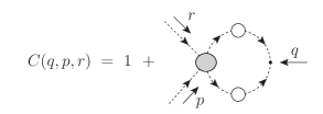
Figure 5: Definitions and conventions of the auxiliary function $C$. The color and coupling dependence for the combination shown, $c^{a}(q)c^{b}(r)c^{*c}(p)$, is $gf^{acb}$. The kernel is one-particle irreducible with respect to vertical cuts

To proceed further, we decompose the auxiliary functions $H$ and $\widetilde{H}$ in terms of their basic tensor forms

$$H_{\nu\mu}(p,r,q) = g_{\mu\nu}a_{qrp}-r_{\mu}q_{\nu}b_{qrp}+q_{\mu}p_{\nu}c_{qrp}+q_{\nu}p_{\mu}d_{qrp}+p_{\mu}p_{\nu}e_{qrp}$$

$$\widetilde{H}_{\nu\mu}(p,r,q) = g_{\mu\nu}\widetilde{a}_{qrp}-r_{\mu}q_{\nu}\widetilde{b}_{qrp}+q_{\mu}p_{\nu}\widetilde{c}_{qrp}+q_{\nu}p_{\mu}\widetilde{d}_{qrp}+p_{\mu}p_{\nu}\widetilde{e}_{qrp},$$ (34)

where, following the notation of Ball:1980ax we have introduced the shorthand notation $a_{qrp}$ for $a(q,r,p)$, and similarly for all other form factors appearing in (34). Then, one can use the identities (29) and (33) in order to constrain certain combinations of these form factors. Indeed from the WI (29) one finds

$$\widetilde{a}_{qrp}-(q\cdot r)\widetilde{b}_{qrp}+(q\cdot p)\widetilde{d}_{qrp} = F^{-1}(r^{2})$$

$$q^{2}\widetilde{c}_{qrp}+(q\cdot p)\widetilde{e}_{qrp}+F^{-1}(p^{2}) = F^{-1}(r^{2}),$$ (35)

while the STI gives

$$F(r^{2})\left[a_{qrp}-(q\cdot r)b_{qrp}+(q\cdot p)d_{qrp}\right] = F(q^{2})\left[a_{rqp}-(q\cdot r)b_{rqp}+(p\cdot r)d_{rqp}\right]$$

$$F^{-1}(q^{2})\left[q^{2}c_{qrp}+(q\cdot p)e_{qrp}\right]+F^{-1}(p^{2})C_{qrp} = F^{-1}(r^{2})\left[a_{rqp}-(q\cdot r)b_{rqp}+(p\cdot r)d_{rqp}\right]$$ (36)

$$- F^{-1}(r^{2})\left[r^{2}c_{rqp}+(p\cdot r)e_{rqp}\right],$$

where, as before, $C_{qrp}\equiv C(q,r,p)$.

The first equation of (36), together with those obtained through cyclic permutations of momenta and indices, represent the aforementioned constraints, first found in Ball:1980ax [viz. Eq. (2.10) in that article] as necessary conditions for solving the STIs of the $QQQ$ vertex. It is clear from the above analysis that these constraints are a direct consequence of the STI satisfied by the function $H$ (in Ball:1980ax their validity was explicitly verified at the one-loop level only).

Finally, let us conclude this section by observing that $H$ and $\widetilde{H}$ can be related. Specificcally, the functional differentiation

$$\left.\frac{\delta^{3}{\cal S}[\Gamma]}{\delta\Omega^{a}_{\alpha}(q)\delta c^{b}(r)\delta A^{*c}_{\nu}(p)}\right|_{\Phi,\Phi^{*},\Omega=0};\qquad q+p+r=0,$$ (37)

furnishes the corresponding BQI, namely

$${i}\Gamma_{c^{b}\widehat{A}^{a}_{\mu}A^{*c}_{\nu}}(r,q,p) = \left[{i}g_{\mu}^{\rho}\delta^{ad}+\Gamma_{\Omega^{a}_{\mu}A^{*\rho}_{d}}(q)\right]\Gamma_{c^{b}A^{d}_{\rho}A^{*c}_{\nu}}(r,q,p)+\Gamma_{c^{b}A^{*\rho}_{d}}(r)\Gamma_{\Omega^{a}_{\alpha}A_{\rho}^{d}A^{*c}_{\nu}}(q,r,p)$$ (38)

$$- \Gamma_{\Omega^{a}_{\mu}c^{b}c^{*d}}(q,r,p)\Gamma_{c^{d}A^{*c}_{\nu}}(p).$$

IV Solving the Ward and Slavnov-Taylor identities

In this section we proceed to the actual construction of the vertex $\widetilde{\mathrm{I}\!\Gamma}$, by solving the WI and STIs given in Eq. (13).

In order to simplify the resulting equations, it is convenient to follow Ball:1980ax and group the 14 possible tensor forms into two sets corresponding to the longitudinal and the (totally) transverse parts of the vertex. One begins by decomposing the vertex according to

$$\widetilde{\mathrm{I}\!\Gamma}^{\alpha\mu\nu}(q,r,p)=\widetilde{\mathrm{I}\!\Gamma}_{(\ell)}^{\alpha\mu\nu}(q,r,p)+\widetilde{\mathrm{I}\!\Gamma}_{(t)}^{\alpha\mu\nu}(q,r,p).$$ (39)

The longitudinal part is then characterized by 10 form factors $X_{i}$ according to

$$\widetilde{\mathrm{I}\!\Gamma}_{(\ell)}^{\alpha\mu\nu}(q,r,p)=\sum_{i=1}^{10}X_{i}(q,r,p)\ell_{i}^{\alpha\mu\nu}(q,r,p),$$ (40)

with the explicit form of the tensors $\ell^{i}$ given by

$$\ell_{1}^{\alpha\mu\nu}=(q-r)^{\nu}g^{\alpha\mu}$$

.

(41)

Notice that excluding $\ell_{10}$, each of the remaining $\ell_{i+3}$ can be obtained by the corresponding $\ell_{i}$ through cyclic permutation of momenta and indices; in addition, Bose symmetry with respect to the quantum legs requires that $\widetilde{\mathrm{I}\!\Gamma}$ reverses sign under the interchange of the corresponding Lorentz indices and momenta, thus implying the relations

$$X_{1}(q,p,r)=X_{7}(q,r,p)$$

(42)

which reduce the number of possible independent form factors from the original 10 to only 7.

The (undetermined) transverse part of the vertex is finally described by the remaining 4 form factors $Y_{i}$

$$\widetilde{\mathrm{I}\!\Gamma}_{(t)}^{\alpha\mu\nu}(q,r,p)=\sum_{i=1}^{4}Y_{i}(q,r,p)t_{i}^{\alpha\mu\nu}(q,r,p),$$ (43)

with the completely transverse tensors $t^{i}$ given by

$$t_{1}^{\alpha\mu\nu} = [(q\cdot r)g^{\alpha\mu}-q^{\mu}r^{\alpha}][(r\cdot p)q^{\nu}-(q\cdot p)r^{\nu}]$$

$$t_{2}^{\alpha\mu\nu} = [(r\cdot p)g^{\mu\nu}-r^{\nu}p^{\mu}][(p\cdot q)r^{\alpha}-(r\cdot q)p^{\alpha}]$$

$$t_{3}^{\alpha\mu\nu} = [(p\cdot q)g^{\nu\alpha}-p^{\alpha}q^{\nu}][(q\cdot r)p^{\mu}-(r\cdot p)q^{\mu}]$$

$$t_{4}^{\alpha\mu\nu} = g^{\mu\nu}[(p\cdot q)r^{\alpha}-(r\cdot q)p^{\alpha}]+g^{\alpha\mu}[(r\cdot p)q^{\nu}-(q\cdot p)r^{\nu}]+g^{\alpha\nu}[(r\cdot q)p^{\mu}-(r\cdot p)q^{\mu}]$$ (44)

$$+ p^{\alpha}q^{\mu}r^{\nu}-r^{\alpha}p^{\mu}q^{\nu}.$$

The form factors $X_{i}$ are then fully determined by solving the system of linear equations generated by the identities given in Eq. (13). The procedure is conceptually straightforward, but operationally rather cumbersome. One first substitutes on the lhs of Eq. (13) the general tensorial decomposition of $\widetilde{\mathrm{I}\!\Gamma}^{(\ell)}$ given in Eq. (40), and then equates the coefficients of the resulting tensorial structures to those appearing on the rhs. Thus, one obtains a system of equations expressing the form factors $X_{i}$ in terms of combinations of quantities such as $J$, $F$, etc.

In what follows we will only report the set of independent equations, i.e., we will omit equations that can be obtained from existing ones by implementing the change $p\leftrightarrow r$ and using the constraints of  (42). Thus, for example, the equation $X_{7}+X_{8}+(q\cdot r)X_{10}=J(p)$ does not form part of the set of independent equations, because it can be obtained from the second equation in Eq.(45) below, by carrying out the aforementioned transformation, and using the corresponding relations from Eq. (42).

Thus, from the Abelian WI one obtains the following 4 equations

$$(p^{2}-r^{2})X_{4}-q^{2}X_{5}-(r\cdot p)(p^{2}-r^{2})X_{6} = p^{2}J(p)-r^{2}J(r)$$

$$X_{1}-X_{2}-(q\cdot p)X_{10} = J(r)$$

$$X_{1}+X_{2}-X_{7}+X_{8} = 0$$

$$2X_{1}+(p^{2}-r^{2})X_{6}-2X_{7}+q^{2}X_{10} = 0,$$ (45)

where the form of the second equation has been simplified by making use of the third.

Similarly, from the non-Abelian STI one obtains

$$(r^{2}-q^{2})X_{1}-p^{2}X_{2}-(q\cdot r)(r^{2}-q^{2})X_{3} = F(p)\left[{\widetilde{a}}_{qpr}r^{2}J(r)-a_{rpq}q^{2}{\widetilde{J}}(q)\right]$$

$$(r^{2}-q^{2})X_{3}-2X_{4}+2X_{7}+p^{2}X_{10} = F(p)\left[({\widetilde{b}}_{qpr}+{\widetilde{d}}_{qpr})r^{2}J(r)-(b_{rpq}+d_{rpq})q^{2}{\widetilde{J}}(q)\right]$$

$$-X_{7}+X_{8}+(r\cdot p)X_{10} = F(p)\left\{(r\cdot p){\widetilde{b}}_{qpr}J(r)-\left[a_{rpq}+(q\cdot r){d}_{rpq}\right]{\widetilde{J}}(q)\right\}$$

$$X_{4}+X_{5}+(q\cdot p)X_{10} = F(p)\left\{\left[{\widetilde{a}}_{qpr}+(q\cdot r){\widetilde{d}}_{qpr}\right]J(r)-(q\cdot p)b_{rpq}{\widetilde{J}}(q)\right\}$$

$$-X_{4}+X_{5}+X_{7}+X_{8} = (q\cdot r)F(p)\left[-{\widetilde{b}}_{qpr}J(r)+b_{rpq}{\widetilde{J}}(q)\right].$$ (46)

Clearly, there are 5 additional equations, obtained from the second STI; however, they too can be obtained from the set of equations (46) by imposing the transformation $r\leftrightarrow p$ and using the relations (42), and are therefore omitted.

Eqs. (45) and (46) furnish a set of 9 equations for the 7 independent longitudinal form factors of Eq. (42); therefore the existence of a (unique) solution to this system, requires the appearance of 2 non-trivial constraints for the ghost sector which read

$$F(r^{2})[{a}_{prq}-(r\cdot p){b}_{prq}+(q\cdot p){d}_{prq}]=F(p^{2})[{a}_{rpq}-(r\cdot p){b}_{rpq}+(q\cdot r){d}_{rpq}]$$

$$F(r^{2})[{\widetilde{a}}_{qrp}-(q\cdot r){\widetilde{b}}_{qrp}+(q\cdot p){\widetilde{d}}_{qrp}]=1.$$ (47)

Evidently these relations are nothing but an expression of the STI and the WI that the ghost auxiliary functions $H$ and $\widetilde{H}$ are bound to satisfy, as shown in Eqs. (35) and (36). Therefore the system can be solved and one finds a solution of the type presented in Ball:1980ax with a modified ghost-sector, reading

$$X_{1}(q,r,p) = \frac{1}{4}{\widetilde{J}}(q)\left\{-p^{2}b_{prq}F(r)+[2a_{rpq}+p^{2}b_{rpq}+2(q\cdot r)d_{rpq}]F(p)\right\}$$

$$+ \frac{1}{4}J(r)\left[2+(r^{2}-q^{2}){\widetilde{b}}_{qpr}F(p)\right]+\frac{1}{4}J(p)\,p^{2}\,{\widetilde{b}}_{qrp}F(r)$$

$$X_{2}(q,r,p) = \frac{1}{4}{\widetilde{J}}(q)\left\{(q^{2}-r^{2})b_{prq}F(r)+[2a_{rpq}+(r^{2}-q^{2})b_{rpq}+2(q\cdot r)d_{rpq}]F(p)\right\}$$

$$+ \frac{1}{4}J(r)\left[-2+p^{2}{\widetilde{b}}_{qpr}F(p)\right]+\frac{1}{4}J(p)\,(r^{2}-q^{2})\,{\widetilde{b}}_{qrp}F(r)$$

$$X_{3}(q,r,p) = \frac{F(p)}{q^{2}-r^{2}}\left\{{\widetilde{J}}(q)\left[a_{rpq}-(q\cdot p)d_{rpq}\right]-J(r)\left[{\widetilde{a}}_{qpr}-(r\cdot p){\widetilde{d}}_{qpr}\right]\right\}$$

$$X_{4}(q,r,p) = \frac{1}{4}{\widetilde{J}}(q)q^{2}\left[b_{prq}F(r)+b_{rpq}F(p)\right]+\frac{1}{4}J(r)\left[2-q^{2}{\widetilde{b}}_{qpr}F(p)\right]$$

$$+ \frac{1}{4}J(p)\left[2-q^{2}{\widetilde{b}}_{qrp}F(r)\right]$$

$$X_{5}(q,r,p) = \frac{1}{4}{\widetilde{J}}(q)(p^{2}-r^{2})\left[b_{prq}F(r)+b_{rpq}F(p)\right]+\frac{1}{4}J(r)\left[2+(r^{2}-p^{2}){\widetilde{b}}_{qpr}F(p)\right]$$

$$- \frac{1}{4}J(p)\left[2+(p^{2}-r^{2}){\widetilde{b}}_{qrp}F(r)\right]$$

$$X_{6}(q,r,p) = \frac{J(r)-J(p)}{r^{2}-p^{2}}$$

$$X_{7}(q,r,p) = X_{1}(q,p,r)$$

$$X_{8}(q,r,p) = -X_{2}(q,p,r)$$

$$X_{9}(q,r,p) = X_{3}(q,p,r)$$

$$X_{10}(q,r,p) = \frac{1}{2}\left\{{\widetilde{J}}(q)\left[b_{prq}F(r)-b_{rpq}F(p)\right]+J(r)F(p){\widetilde{b}}_{qpr}-J(p)F(r){\widetilde{b}}_{qrp}\right\}.$$ (48)

Notice finally that from the above result one can obtain also the solution for the fully Bose-symmetric PT vertex $\widehat{\bm{\Gamma}}$, namely the $BBB$ vertex originally constructed in Cornwall:1989gv , and further studied in Binger:2006sj . This vertex satisfies (with respect to any one of its three-legs) the WI shown in the first line of (13), with the modification $\Delta^{-1}\to\widehat{\Delta}^{-1}$, where

$$\widehat{\Delta}^{-1}(q^{2})=q^{2}\widehat{J}(q^{2});\qquad\widehat{J}(q^{2})=[1+G(q^{2})]^{2}J(q^{2}),$$ (49)

is the inverse of the full PT-BFM gluon propagator. Thus, from the STIs appearing in Eq. (13) we see that the expression for the (longitudinal part) of the $BBB$ vertex (given in Binger:2006sj ) may be recovered from Eq. (48) by setting $J,\widetilde{J}\to\widehat{J}$, $F=1$ and $a=\widetilde{a}=1$, and all remaining form factors of $H$ and $\widetilde{H}$ equal to zero.

V Consequences for the SDE of the gluon propagator

As has already been mentioned in previous sections, the Ansatz for the longitudinal part of the $BQQ$ vertex, obtained by “solving” the WI and STI that this vertex satisfies, is of central importance for the self-consistent treatment of the SDE equation governing the dynamics of the gluon self-energy. This fact may be best appreciated in the context of the SDE governing the gluon propagator (7) projected onto the Landau gauge, which is known to display a variety of field-theoretic subtleties.

In particular, a crucial self-consistency condition for the mechanism of dynamical gluon mass generation developed in a series of articles Cornwall:1981zr ; Aguilar:2006gr ; Binosi:2007pi ; Binosi:2008qk ; Aguilar:2008xm is the cancellation of all seagull-type of divergences, i.e., divergences produced by integrals of the type $\int_{k}\Delta(k)$, or variations thereof Aguilar:2009ke . In the case of the dimensional regularization that we use throughout, the presence of such integrals would give rise to divergences of the type $m_{0}^{2}(1/\epsilon)$, where $m_{0}$ is the value of the dynamically generated gluon mass at $q^{2}=0$, i.e., $m_{0}=m(0)$; if a hard cutoff $\Lambda$ were to be employed, these latter terms would diverge quadratically, as $\Lambda^{2}$. The disposal of such divergences would require the introduction in the original Lagrangian of a counter-term of the form $m^{2}_{0}A^{2}_{\mu}$, which is, however, forbidden by the local gauge invariance, which must remain intact.

This is a point of paramount importance. Indeed, in the picture put forth in the aforementioned articles, the Lagrangian of the Yang-Mills theory (or that of QCD) is never altered; the generation of the gluon mass takes place dynamically, without violating any of the underlying symmetries. Amplifying this point further, let us mention that, given that the Lagrangian is never altered, the only other possible way of violating the gauge (or BRST) symmetry would be by not respecting, at some intermediate step, some of the WIs and STIs satisfied by the Green’s functions involved; for example, in the conventional SDE formulation, a naive truncation would compromise the transversality of the resulting gluon self-energy, i.e., the text-book condition $q^{\mu}\Pi_{\mu\nu}(q)=0$ would be no longer valid.

Returning to the aforementioned seagull-type of divergences, as has been shown in detail in Aguilar:2009ke , their cancellation proceeds by means of the identity

$$\int_{k}\!k^{2}\frac{\partial{\Delta}(k^{2})}{\partial k^{2}}+\frac{d}{2}\int_{k}\!\Delta(k^{2})=0,$$ (50)

whose validity hinges on the special rules of dimensional regularization. In fact, as explained in  Aguilar:2009ke , in scalar QED it is exactly this identity that enforces the masslessness of the photon both perturbatively (at the level of a one-loop calculation) as well as non-perturbatively, at the level of the one-loop dressed SDE (assuming that the Schwinger mechanism is not in operation). In this context, the difference between scalar QED and Yang-Mills is that in the former case $\Delta$ should be replaced by the propagator of the charged scalar field ${\cal D}$ entering into the loop of the photon self-energy, whereas in the latter, $\Delta$ is the gluon propagator itself (entering in its own gluonic loop, see Fig. 2). Note that the two types of integrals appearing on the lhs of Eq. (50) are individually non-vanishing (in fact, they both diverge); it is only when they come in the particular combination shown above that they sum up to zero.

The difficulty associated with Eq. (50) is not so much recognizing its validity, but rather, having it triggered at the end of the calculation. Specifically, the ingredients entering into the SDE (most importantly, the vertex) must be such that, after taking the limit of the SDE as $q\to 0$, all seagull-type contributions must conspire to appear in the combination given on the lhs of Eq. (50) only! In fact, the slightest change in a relative numerical factor will invalidate the entire construction.

Let us now see in detail how this seagull cancellation proceeds in the case of the Landau gauge SDE, supplied with the $BQQ$ vertex constructed earlier. The gluon self-energy obtained from the PT-BFM one-loop dressed SDE (see Fig. 2) in the Landau gauge reads

$${\widehat{\Pi}}^{\mu\nu}(q)=g^{2}C_{A}\sum_{i=1}^{5}A^{\mu\nu}_{i}(q),$$ (51)

with

$$A^{\mu\nu}_{1}(q) = \frac{1}{2}\int_{k}\Gamma^{(0)\mu}_{\alpha\beta}\Delta^{\alpha\rho}_{t}(k)\Delta^{\beta\sigma}_{t}(k+q)\widetilde{\mathrm{I}\!\Gamma}^{\nu}_{\rho\sigma}$$

$$A^{\mu\nu}_{2}(q) = \int_{k}\!\Delta^{\alpha\mu}_{t}(k)\frac{(k+q)^{\beta}\Gamma^{(0)\nu}_{\alpha\beta}}{(k+q)^{2}}$$

$$A^{\mu\nu}_{3}(q) = \int_{k}\!\Delta^{\alpha\mu}_{t}(k)\frac{(k+q)^{\beta}\widetilde{\mathrm{I}\!\Gamma}^{\nu}_{\alpha\beta}}{(k+q)^{2}}$$

$$A^{\mu\nu}_{4}(q) = -\frac{(d-1)^{2}}{d}g^{\mu\nu}\int_{k}\Delta(k)$$

$$A^{\mu\nu}_{5}(q) = \int_{k}\frac{k^{\mu}(k+q)^{\nu}}{k^{2}(k+q)^{2}},$$ (52)

and $\Delta_{t}^{\mu\nu}(q)=P^{\mu\nu}(q)\Delta(q^{2})$ is the transverse Landau gauge propagator.

First of all, it is rather straightforward to verify explicitly that, if $\widetilde{\mathrm{I}\!\Gamma}$ satisfies the WI of Eq. (13),

$$q^{\mu}{\widehat{\Pi}}_{\mu\nu}(q)=0.$$ (53)

Therefore, ${\widehat{\Pi}}^{\mu\nu}(q)=P^{\mu\nu}(q)\widehat{\Pi}(q^{2})$, and the scalar function $\widehat{\Pi}(q^{2})$ is given by

$$\widehat{\Pi}(q^{2})=\frac{g^{2}C_{A}}{d-1}\sum_{i=1}^{5}A_{i\,\mu}^{\mu}(q).$$ (54)

Since we are interested in the behavior of $\widehat{\Pi}(0)$, and in particular the annihilation of any seagull-type of divergence, we next take the limit $q\to 0$ of the rhs of Eq. (54), using the explicit form of the vertex $\widetilde{\mathrm{I}\!\Gamma}$ derived in the preceding section. In addition, we will assume that all form factors appearing in the Lorentz decomposition of $H$ and $\widetilde{H}$ are regular in the $q\to 0$ limit; this is a reasonable assumption, given that the generation of a dynamical mass is expected to regulate all potential infrared divergences.

Consider then the term $A_{1}$; after replacing $r\to k$ and $p\to-k-q$, and dropping terms proportional to $k_{\rho}$ and $(k+q)_{\sigma}$, given that they vanish when contracted with the corresponding transverse propagators, we find that the tensor structures $\ell_{i}$ are such that

$$\ell_{1}^{\beta\rho\sigma}\sim\ell_{5}^{\beta\rho\sigma}\sim\ell_{7}^{\beta\rho\sigma}\sim{\cal O}(q);\qquad\ell_{3}^{\beta\rho\sigma}\sim\ell_{9}^{\beta\rho\sigma}\sim{\cal O}(q^{2});\qquad\ell_{10}^{\beta\rho\sigma}\sim{\cal O}(q^{3}).$$ (55)

Since $\ell_{2}$ and $\ell_{8}$ yield a vanishing result when contracted with the transverse propagators, the only tensors surviving will be $\ell_{4}$ and $\ell_{6}$; after taking the trace, one is then left with the result

$$A_{1}=2(d-1)\int_{k}\!k^{2}\Delta(k)\Delta(k+q)\left[X_{4}+k\cdot(k+q)X_{6}\right]+{\cal O}(q).$$ (56)

On the other hand, using the explicit results given in Eq. (48), one has

$$X_{4}+k\cdot(k+q)X_{6}=\frac{\Delta^{-1}(k+q)-\Delta^{-1}(k)}{(k+q)^{2}-k^{2}}-\frac{q^{2}}{2}\frac{J(k+q)-J(k)}{(k+q)^{2}-k^{2}},$$ (57)

and the second term is easily shown to vanish as $q$ goes to zero. Thus, one is finally left with the result

$$A_{1}=-2(d-1)\int_{k}\!k^{2}\frac{\Delta(k+q)-\Delta(k)}{(k+q)^{2}-k^{2}}+{\cal O}(q).$$ (58)

Thus, in the limit $q\to 0$ one obtains

$$\frac{\Delta(k+q)-\Delta(k)}{(k+q)^{2}-k^{2}}=\frac{\partial{\Delta}(k^{2})}{\partial k^{2}}+{\cal O}(q^{2}),$$ (59)

which gives rise to the first term on the lhs of Eq. (50).

The second contribution to Eq. (50) arises from two terms, the obvious term $A_{4}$, which already has the required form (but not the right numerical coefficient), and the term $A_{2}$, which, after letting the momentum $(k+q)^{\beta}$ act on the tree-level vertex $\Gamma^{(0)\nu}_{\alpha\beta}$, reads

$$A_{2}=-(d-1)\int_{k}\Delta(k)+{\cal O}(q).$$ (60)

Putting all pieces together, we finally obtain

$$A_{1}+A_{2}+A_{4} = -2\left[\int_{k}\!k^{2}\frac{\Delta(k+q)-\Delta(k)}{(k+q)^{2}-k^{2}}+\frac{d}{2}\int_{k}\!\Delta(k)\right]+\mathcal{O}(q)$$ (61)

$$\stackrel{{\scriptstyle q\to 0}}{{\longrightarrow}} -2\left[\int_{k}\!k^{2}\frac{\partial{\Delta}(k^{2})}{\partial k^{2}}+\frac{d}{2}\int_{k}\!\Delta(k)\right]=0,$$

that is, one recovers the seagull cancellation condition of Eq. (50).

Let us finally look at what happens to the remaining terms $A_{3}$ and $A_{5}$ as $q\to 0$. To begin with, it is elementary to check that $A_{5}(0)=0$. The treatment of $A_{3}$ is more subtle, and makes manifest the need to satisfy the STI of Eq. (13). Specifically, after taking the trace and using Eq. (13), one finds

$$A_{3} = -\int_{k}\!\Delta_{t}^{\mu\rho}(k)\frac{F(k+q)}{(k+q)^{2}}\bigg{[}\Delta^{-1}(k)P_{\rho}^{\sigma}(k)\widetilde{H}_{\sigma\mu}(k,-k-q,q)$$ (62)

$$- \widetilde{\Delta}^{-1}(q)P^{\sigma}_{\rho}(q)H_{\sigma\mu}(q,-k-q,k)\bigg{]}.$$

Substituting the expansion for $\widetilde{H}$ given in Eq. (34), the first term on the rhs of Eq. (62) yields

$$-\int_{k}\!\frac{F(k+q)}{(k+q)^{2}}P^{\mu\sigma}(k)\left[g_{\mu\sigma}\widetilde{a}+(k+q)_{\mu}q_{\sigma}\widetilde{b}\right],$$ (63)

where the argument of the form factors $\widetilde{a}$ and $\widetilde{b}$ is now $(q,-k-q,k)$. In the $q\to 0$ limit this term vanishes in dimensional regularization, by virtue of the well-known property $\int_{k}k^{-2}=0$. Indeed,

$$\int_{k}\!\frac{F(k)}{k^{2}}\widetilde{a}(0,-k,k)=\int_{k}\!\frac{1}{k^{2}}=0,$$ (64)

where we have used the fact that, in this limit, the first equation of (35) reduces to the simple relation

$$\widetilde{a}(0,-k,k)=F^{-1}(k).$$ (65)

Next, consider the second term in Eq. (62); using now the expansion (34) for $H$, we obtain

$$\widetilde{\Delta}^{-1}(q)\int_{k}\!\Delta(k)\frac{F(k+q)}{(k+q)^{2}}P_{\mu}^{\rho}(k)P^{\mu\sigma}(q)\left[g_{\rho\sigma}a-(k+q)_{\rho}k_{\sigma}b+k_{\sigma}q_{\rho}d\right],$$ (66)

where now the form factors $a$, $b$ and $d$ carry the argument $(k,-k-q,q)$. In the $q\to 0$ limit this integral gives a finite term, proportional to the expression

$$\int_{k}\!\Delta(k)\frac{F(k)}{k^{2}}a(k,-k,0).$$ (67)

It should be noticed that the contribution of the term $A_{3}$ is rendered finite precisely by virtue of the special properties of the ghost sector. In fact, if one were to use in the SDE the fully Bose-symmetric PT vertex $BBB$ (instead of the correct $BQQ$ vertex that we use here), the term $A_{3}$ would give rise to an ultraviolet divergence, since (as explained at the end of the previous section) one should set in (67) $F,a\to 1$.

These observations demonstrate that, as happens in the case of chiral symmetry breaking  Aguilar:2010cn , the complete treatment of the ghost dynamics is instrumental also for the self-consistency of the mass generation in the purely gluonic sector of QCD.

VI Conclusions

In this article we have constructed a gauge technique inspired Ansatz for the $BQQ$ three-gluon vertex $\widetilde{\mathrm{I}\!\Gamma}$ that naturally arises in the context of the PT-BFM derivation of the SDE equations for Yang-Mills theories. An indispensable step for realizing this construction has been the formal derivation within the Batalin-Vilkovisky formalism of the all-order WI (respectively STI) satisfied by the ghost Green’s functions $\widetilde{H}$ (respectively $H$), which, as shown in Section IV, furnish crucial constraints that allow $\widetilde{\mathrm{I}\!\Gamma}$ to conform with both the WI as well as the STIs of Eq. (13).

It is important to emphasize that the analysis presented here is completely general, and in particular that the solution shown in Eq. (48) is valid irrespectively of the value of the gauge-fixing parameter used to quantize the theory. To be sure, the various ingredients appearing in Eq. (48), such as $J$, $F$, etc., depend explicitly on $\xi$ (or on $\xi_{Q}$); nevertheless, the precise functional dependence of the form factors $X_{i}$ on these functions, is always valid, given that it originates from the solution of the WI and STIs (13), whose form is in turn gauge fixing parameter independent. This is particularly relevant, given the existing perspectives Cucchieri:2009kk ; Cucchieri:2011aa of carrying out large-volume lattice simulations of the gluon and ghost propagators in covariant gauges other than the Landau gauge, i.e., at $\xi\neq 0$. In particular, the possibility of simulating propagators in background-type gauges (especially the background Feynman gauge, $\xi_{Q}=1$) opens up the interesting prospect of studying central quantities of the PT-BFM approach directly on the lattice Cucchieri:2011aa .

As already mentioned in the Introduction, the construction based on solving the WI and STI leaves the transverse part of the vertex undetermined. In terms of the notation introduced in section IV, this means that the four form factors $Y_{i}$ appearing in Eq. (43) are completely unconstrained. In the case of QED, it is known that, in the presence of a mass gap, the transverse part of the photon-electron vertex is sub-leading in the infrared. Even though we are not aware of a similar study in a non-Abelian context, it is reasonable to assume that this will continue to be so, provided that a mass gap (i.e., dynamical gluon mass) has indeed been generated. In such a case, one would expect that the identically conserved part of the vertex should vanish more rapidly by at least one power of $q$ compared to the longitudinal part, leaving the infrared dynamics largely unaffected. On the other hand, this ambiguity affects the ultraviolet properties of the SDEs Salam:1963sa ; Salam:1964zk ; Delbourgo:1977jc ; Delbourgo:1977hq . Essentially, failing to provide the correct transverse part leads to the mishandling of overlapping divergences, which, in turn, compromises the multiplicative renormalizability of the resulting SD equations. The construction of the appropriate transverse part is technically complicated, even for QED King:1982mk ; Curtis:1990zs ; Kizilersu:2009kg ; Bashir:1997qt , and its systematic generalization to QCD is still pending (for an early attempt in this direction, see Haeri:1988af ).

An additional important point, not addressed here, is related to the way the $BQQ$ vertex triggers the Schwinger mechanism Schwinger:1962tn ; Schwinger:1962tp , which, in turn, is responsible for the dynamical generation of a gluon mass. As is well-known Jackiw:1973tr ; Cornwall:1973ts ; Eichten:1974et , the relevant three-gluon vertex ($\widetilde{\mathrm{I}\!\Gamma}$ in this case) must contain longitudinally coupled massless poles (last diagram in Fig. 3), in order for gauge invariance to be preserved. The Ansatz presented here does not incorporate such poles, which must be supplied at a subsequent step; after this has been accomplished, one can solve numerically the resulting SDE, and compare with the available lattice results. Work in this direction is currently underway, and we hope to report on the results in the near future.

- (1) A. Cucchieri and T. Mendes, PoS LAT2007, 297 (2007).
- (2) A. Cucchieri and T. Mendes, Phys. Rev. Lett. 100, 241601 (2008).
- (3) A. Cucchieri and T. Mendes, Phys. Rev. D 81, 016005 (2010).
- (4) A. Cucchieri and T. Mendes, PoS LATTICE2010, 280 (2010).
- (5) A. Cucchieri and T. Mendes, arXiv:1101.4779 [hep-lat].
- (6) I. L. Bogolubsky, E. M. Ilgenfritz, M. Muller-Preussker and A. Sternbeck, PoS LATTICE, 290 (2007).
- (7) P. O. Bowman et al., Phys. Rev. D 76, 094505 (2007).
- (8) I. L. Bogolubsky, E. M. Ilgenfritz, M. Muller-Preussker and A. Sternbeck, Phys. Lett. B 676, 69 (2009).
- (9) O. Oliveira and P. J. Silva, PoS LAT2009, 226 (2009).
- (10) A. C. Aguilar and J. Papavassiliou, JHEP 0612, 012 (2006).
- (11) D. Binosi and J. Papavassiliou, Phys. Rev. D 77(R), 061702 (2008).
- (12) D. Binosi and J. Papavassiliou, JHEP 0811, 063 (2008).
- (13) J. M. Cornwall, Phys. Rev. D 26, 1453 (1982).
- (14) J. M. Cornwall and J. Papavassiliou, Phys. Rev. D 40, 3474 (1989).
- (15) D. Binosi and J. Papavassiliou, Phys. Rev. D 66(R), 111901 (2002).
- (16) D. Binosi and J. Papavassiliou, J. Phys. G 30, 203 (2004).
- (17) D. Binosi and J. Papavassiliou, Phys. Rept. 479, 1-152 (2009).
- (18) See, e.g., L. F. Abbott, Nucl. Phys. B 185, 189 (1981), and references therein.
- (19) R. Alkofer, L. von Smekal, Phys. Rept. 353, 281 (2001).
- (20) C. S. Fischer, J. Phys. G 32, R253 (2006).
- (21) D. Dudal, J. A. Gracey, S. P. Sorella, N. Vandersickel and H. Verschelde, Phys. Rev. D 78, 065047 (2008).
- (22) Ph. Boucaud, J. P. Leroy, A. L. Yaouanc, J. Micheli, O. Pene and J. Rodriguez-Quintero, JHEP 0806 (2008) 012.
- (23) J. Braun, H. Gies and J. M. Pawlowski, Phys. Lett. B 684, 262 (2010).
- (24) A. P. Szczepaniak and H. H. Matevosyan, Phys. Rev. D 81, 094007 (2010).
- (25) J. Rodriguez-Quintero, PoS LC2010, 023 (2010).
- (26) J. Rodriguez-Quintero, arXiv:1012.0448 [hep-ph].
- (27) A. C. Aguilar, J. Papavassiliou, Phys. Rev. D81, 034003 (2010).
- (28) A. Salam, Phys. Rev. 130, 1287 (1963).
- (29) A. Salam and R. Delbourgo, Phys. Rev. 135, B1398 (1964).
- (30) R. Delbourgo and P. C. West, J. Phys. A 10, 1049 (1977).
- (31) R. Delbourgo and P. C. West, Phys. Lett. B 72, 96 (1977).
- (32) J. S. Ball and T. W. Chiu, Phys. Rev. D 22, 2550 (1980) [Erratum-ibid. D 23, 3085 (1981)].
- (33) A. I. Davydychev, P. Osland and O. V. Tarasov, Phys. Rev. D 54, 4087 (1996) [Erratum-ibid. D 59, 109901 (1999)]
- (34) A. Pilaftsis, Nucl. Phys. B 487, 467 (1997)
- (35) J. S. Schwinger, Phys. Rev. 125, 397 (1962).
- (36) J. S. Schwinger, Phys. Rev. 128, 2425 (1962).
- (37) R. Jackiw and K. Johnson, Phys. Rev. D 8, 2386 (1973).
- (38) J. M. Cornwall and R. E. Norton, Phys. Rev. D 8 (1973) 3338.
- (39) E. Eichten and F. Feinberg, Phys. Rev. D 10, 3254 (1974).
- (40) J. S. Ball and T. W. Chiu, Phys. Rev. D 22, 2542 (1980).
- (41) A. C. Aguilar, D. Binosi and J. Papavassiliou, Phys. Rev. D 78, 025010 (2008).
- (42) P. A. Grassi, T. Hurth and M. Steinhauser, Annals Phys. 288, 197 (2001).
- (43) D. Binosi and J. Papavassiliou, Phys. Rev. D 66, 025024 (2002).
- (44) I. A. Batalin, G. A. Vilkovisky, Phys. Lett. B69, 309-312 (1977).
- (45) I. A. Batalin, G. A. Vilkovisky, Phys. Lett. B102, 27-31 (1981).
- (46) M. Binger and S. J. Brodsky, Phys. Rev. D 74, 054016 (2006)
- (47) A. C. Aguilar and J. Papavassiliou, Phys. Rev. D 83, 014013 (2011).
- (48) A. Cucchieri, T. Mendes and E. M. S. Santos, Phys. Rev. Lett. 103, 141602 (2009).
- (49) A. Cucchieri, T. Mendes and G. M. N. Santos, arXiv:1101.5080 [hep-lat].
- (50) J. E. King, Phys. Rev. D 27, 1821 (1983).
- (51) D. C. Curtis and M. R. Pennington, Phys. Rev. D 42, 4165 (1990).
- (52) A. Kizilersu and M. R. Pennington, Phys. Rev. D 79, 125020 (2009).
- (53) A. Bashir, A. Kizilersu and M. R. Pennington, Phys. Rev. D 57, 1242 (1998).
- (54) B. J. Haeri, Phys. Rev. D 38, 3799 (1988).