Shock waves in cosmic strings: growth of current

Abstract

Intrinsic equations of motion of superconducting cosmic string may admit solutions in the shock-wave form that implies discontinuity of the current term $\chi$. The hypersurface of discontinuity propagates at finite velocity determined by finite increment $\Delta\chi=\chi_{+}-\chi_{-}$. The current increases $\chi_{+}>\chi_{-}$ in stable shocks but transition between spacelike ($\chi>0$) and timelike ($\chi<0$) currents is impossible.

1 Introduction

Cosmic strings are 2-dimensional topological defects that may be formed at a phase transition in the early universe [1, 2]. Although their direct detection is still impossible with modern technical equipment, they are believed to be responsible for several astrophysical phenomena associated with gravitational lensing, gravitational waves, particle acceleration and gamma-ray bursts [3, 4], and their theoretical study can give better understanding of the global structure of the universe.

The dynamics cosmic strings is determined by the Lagrangian $\Lambda$, also called as equation of state (EOS). The Lagrangian of the Goto-Nambu model $\Lambda=-m^{2}$ depends on the only mass parameter $m$. Cosmic strings may have non-trivial internal structure, giving rise to additional degrees of freedom associated, for example, with transversal oscillations of the worldsheet, or actual particles (bosons or fermions) trapped in the defect core [5]. Such current-carrying or ”superconducting” strings are described by the Lagrangian $\Lambda=\Lambda(m,\chi)$ which depends on the magnitude of the current $\chi=-h^{ab}\partial\phi/\partial\sigma^{a}\partial\phi/\partial\sigma^{b}$ that includes the surface metric $h^{ab}$ with respect to local coordinates $\sigma^{a}$ within the string worldsheet, and the scalar field $\phi$ coupled to the string.

There are only few explicit analytical models of superconducting strings. The linear EOS [6] $\Lambda=-m^{2}-\chi/2$ is applied to the strings that carry fermionic currents. Bosonic current carriers are described by much more complicated EOS, namely, the ”transonic” model [7, 8, 9]

$$\Lambda=-m\sqrt{m^{2}+\chi}$$ (1)

the ”polynomial” model [10]:

$$\Lambda=-m^{2}-\frac{\chi}{2}\left(1+\frac{\chi}{m_{*}^{2}}\right)$$ (2)

the ”rational” model [11, 12]:

$$\Lambda=-m^{2}-\frac{\chi}{2}\left(1+\frac{\chi}{m_{*}^{2}}\right)^{-1}$$ (3)

and the ”logarithmic” model [10, 13]:

$$\Lambda=-m^{2}-\frac{m_{*}^{2}}{2}\ln\left(1+\frac{\chi}{m_{*}^{2}}\right)$$ (4)

where additional mass parameter $m_{*}$ is introduced.

In contrast to the Goto-Nambu model, the superconducting string models admit a large variety of stable loop solutions (or, vortons) and their intercommutation may frequently take place [14, 15]. The problem of vorton stability and evolution of superconducting string networks attract the interest of researchers because such string loops can accumulate significant part of the universe mass and the expected dominant effect of their reconnection is particle radiation (when some particles are expelled away).

The equations of motion of superconducting strings admit solutions in the form of infinitesimal perturbations of two types [16]: extrinsic (transverse) perturbations of the worldsheet that are oscillations of the string geometry, and intrinsic (longitudinal) perturbations within the worldsheet that are oscillations of the current $\chi$. However, this equilibrium, or so-called ”elastic” description is admitted until small transverse oscillations grow up and form abrupt changes in the geometry (kinks), or when small longitudinal oscillations are accumulated into finite-amplitude discontinuities of the current (shock waves) [17, 18]. Such strings loops may tend to fold on themselves and make contact points of self-intersection so that it will be energetically favored to some of the trapped particles to move out of the string, thus, generating emission, associated with possible visible consequences [1, 2, 3, 4].

The dynamical evolution of a fermionic current carrier can develop only kinks, while a bosonic current carrier can develop kinks at time-like (or ”electric”) currents $\chi<0$ and shocks at space-like (or ”magnetic”) currents $\chi>0$ [17, 18]. In the latter case nonlinear effects become dominant rapidly in longitudinal perturbations and a stable discontinuity appears: the magnitude $\chi$ becomes discontinuous and the total energy is no longer conserved. This singular behavior of superconducting strings cannot be assigned to some projection effect because it is seen in simple analytical analysis [19] as well as it is observed in numerical simulations performed both in two dimensions [17] and in three dimensions [18]. An evident hint to a shock wave can be also recognized in numerical simulation of a 2-dimensional vorton in the magnetic regime (Figure 7 in Ref. [20]).

In the present paper we complete the analytical analysis of shocks in superconducting cosmic strings. Particular interest is focused on the behavior of the bosonic current, the shock velocity, the transition between electric and magnetic regimes.

2 Small perturbations and shocks

The physical behavior of superconducting strings is described by the equations of motion. Their projection along the string worldsheet yields the ’intrinsic’ equations or the conservation laws [16]

$$\eta_{\mu}^{\nu}\nabla_{\nu}\,j^{\mu}=0$$ (5)

for $j^{\mu}=\mu v^{\mu}$ and $j^{\mu}=nv^{\mu}$ where tensor $\eta_{\mu}^{\nu}=v^{\nu}v_{\mu}-u^{\nu}u_{\mu}$ is composed of mutually orthogonal unit vectors ($u^{\mu}u_{\mu}=-1=-v^{\mu}v_{\mu}$ and $u^{\mu}v_{\mu}=0$), and dynamical parameters [11]

$$\begin{array}[]{c}\mu^{2}=\chi\qquad n^{2}=K^{2}\chi\qquad\chi>0\\ \mu^{2}=-K^{2}\chi\qquad n^{2}=-\chi\qquad\chi<0\end{array}$$ (6)

are determined by function [10]

$$K=-\frac{1}{2}\left(\frac{d\Lambda}{d\chi}\right)^{-1}$$ (7)

The longitudinal or ’sound’ perturbations run within the worldsheet at velocity [16] $c^{2}=c_{L}^{2}=\left(n/\mu\right)d\mu/dn$ that in the light of (6)-(7) is written in the form

$$c^{2}=\left(1+2\frac{\chi}{K}\frac{dK}{d\chi}\right)^{\mp 1}$$ (8)

where the upper (lower) signs correspond to $\chi>0$ ($\chi<0$). It is always $K<1$ at $\chi<0$, $K\left(0\right)=1$ and $K>1$ at $\chi>0$ because $dK/d\chi>0$ for all known models (1)-(3) .

According to the linear EOS of fermionic cosmic strings $\Lambda=-m^{2}-\chi/2$, the sound speed (8) coincides with the speed of light $c=c_{light}=1$. The bosonic string models (1)-(3) are endowed with finite sound speed dispersion $dc/d\chi\neq 0$ that provides a possibility for development of shock waves [19]. As a matter of fact, the fermionic current-carrying strings can develop only kinks, while the bosonic strings admit both kinks and shocks [17, 18].

The front of a shock wave is a hypersurface in 4-dimensional space whose equation is given in the form $\phi\left(x\right)=0$. It implies that $\phi_{+}\equiv\phi_{-}$ for any two points in the hypersurface but, in general, $\phi_{+}-\phi_{-}\neq 0$ for arbitrary two points beyond the hypersureface, particularly, when ”$-$” and ”$+$” label the states before and behind the front. A stable shock front is associated with characteristic space-like vector

$$\lambda_{\nu}\equiv\frac{d\phi}{dx_{\nu}}$$ (9)

which is the same before and behind the front $\lambda_{+\nu}=\lambda_{-\nu}=\lambda_{\nu}$. It can be presented in the basis $\left(u_{\nu},v_{\nu}\right)$ in the following form

$$\lambda_{-\nu}=\frac{w_{-}u_{-\nu}+v_{-\nu}}{\sqrt{1-w_{-}^{2}}}\qquad\lambda_{+\nu}=\frac{w_{+}u_{+\nu}+v_{+\nu}}{\sqrt{1-w_{+}^{2}}}$$ (10)

where parameters $w_{-}$ and $w_{+}$ play the role of velocities whose essence is clarified below.

All dynamical variables in the intrinsic equations of motion (5) are dependent on function $\phi\left(x\right)$, and, crossing the discontinuity, we have [21]

$$\eta_{+\mu}^{\nu}\nabla_{\nu}j_{+}^{\mu}=\eta_{-\mu}^{\nu}\nabla_{\nu}j_{-}^{\mu}+\left[\eta_{\mu}^{\nu}\nabla_{\nu}j^{\mu}\right]$$ (11)

where square brackets imply a jump of parameters across the discontinuity. In the light of (5), equation (11) implies

$$\left[\eta_{\mu}^{\nu}\frac{Dj^{\mu}}{d\phi}\frac{d\phi}{dx^{\nu}}\right]=\left[\lambda_{\mu}\frac{Dj^{\mu}}{d\phi}\right]=\lambda_{\mu}\frac{\,j_{+}^{\mu}-\,j_{-}^{\mu}}{\phi_{+}-\phi_{-}}=\frac{\lambda_{+\mu}\,j_{+}^{\mu}-\lambda_{-\mu}\,j_{-}^{\mu}}{\phi_{+}-\phi_{-}}=0$$ (12)

and at finite $\phi_{+}-\phi_{-}\neq 0$ it yields relation at the front $\lambda_{+\mu}\,j_{+}^{\mu}=\lambda_{-\mu}\,j_{-}^{\mu}$ , that implies $\lambda_{+\mu}\,\mu_{+}v_{+}^{\mu}=\lambda_{-\mu}\,\mu_{-}v_{-}^{\mu}$ and $\lambda_{+\mu}\,n_{+}u_{+}^{\mu}=\lambda_{-\mu}\,n_{-}u_{-}^{\mu}$. Taking (10), we find the shock parameters

$$w_{-}^{2}=\frac{n_{+}^{2}}{\mu_{+}^{2}}\frac{\mu_{+}^{2}-\mu_{-}^{2}}{n_{+}^{2}-n_{-}^{2}}\qquad w_{+}^{2}=\frac{n_{-}^{2}}{\mu_{-}^{2}}\frac{\mu_{+}^{2}-\mu_{-}^{2}}{n_{+}^{2}-n_{-}^{2}}$$ (13)

Consider a discontinuity in the the laboratory reference frame (see scheme in Fig. 1a) and, altogether, in the reference frame, co-moving its front (see Fig. 1b). The front is at rest and the flow before it has finite velocity, say, $w_{-}$, while the flow behind the front has velocity $w_{+}$. When we turn to the laboratory reference frame (Fig. 1a), the shock-wave propagates along the string at velocity $D_{-}=-w_{-}$, while the velocity behind the front $D_{+}=(w_{+}-w_{-})/(1-w_{-}\,w_{+})$ is finite if $w_{+}\neq w_{-}$. Formula (13) yields $w_{-}\rightarrow$ $w_{+}$ $\rightarrow$ $c$ in the sound limit $n_{+}\rightarrow n_{-}$ and $\mu_{+}\rightarrow\mu_{-}$. Hence, $D_{-}=-c$ and $D_{+}=0$ corresponds to a sound wave (8) because no material flow is generated behind the shock.

Taking $\mu$ and $n$ from equation (6), we determine the shock wave velocity in the magnetic regime ($\chi>0$):

$$w_{-}^{2}=w_{+}^{2}\frac{K_{+}^{2}}{K_{-}^{2}}=K_{+}^{2}\frac{\chi_{+}-\chi_{-}}{K_{+}^{2}\chi_{+}-K_{-}^{2}\chi_{-}}$$ (14)

and in the electric regime ($\chi<0$):

$$w_{-}^{2}=w_{+}^{2}\frac{K_{-}^{2}}{K_{+}^{2}}=\frac{1}{K_{+}^{2}}\frac{K_{+}^{2}\chi_{+}-K_{-}^{2}\chi_{-}}{\chi_{+}-\chi_{-}}$$ (15)

3 Growth of current

Existence of a stable shock is possible when the evolutionary condition is satisfied [22, 23]. For the shock waves in strings it implies [19]:

$$w_{-}>c_{-}\qquad w_{+}<c_{+}$$ (16)

that coincides with the same criterion for the ordinary shock waves. However, this fact can be predicted immediately by means of very easy analysis. The number of intrinsic equations of motion (5) for $j^{\mu}=\mu v^{\mu}$ and $j^{\mu}=nv^{\mu}$ is two, while there is only one material parameter $\chi$: hence, the shock in a string has exactly one degree of freedom. The shock waves in continuous medium are described by three independent equations of motion [22, 23], while there are two material parameters (the pressure and entropy), and, again, there is only one degree of freedom. It implies that the shocks in fluids and cosmic strings obey the same constraint (16), imposed on their velocities.

Now consider small-amplitude shock waves. If increment $\Delta\chi=\chi_{+}-\chi_{-}$ is small with respect to $\left|\chi_{\pm}\right|$, formulas (14)- (15) can be expanded in a series of $\Delta\chi$. According to (14)-(15), we have

$$\frac{w_{-}^{2}}{c_{-}^{2}}-1=1-\frac{w_{+}^{2}}{c_{+}^{2}}=c_{-}^{2}\frac{Q}{K_{-}^{2}}\chi_{-}\Delta\chi\qquad\chi_{-}>0$$ (17)

$$\frac{w_{-}^{2}}{c_{-}^{2}}-1=1-\frac{w_{+}^{2}}{c_{+}^{2}}=-\frac{1}{c_{-}^{2}}\frac{Q}{K_{-}^{2}}\chi_{-}\Delta\chi\qquad\chi_{-}<0$$ (18)

where

$$Q=3\left(\frac{dK}{d\chi}\right)^{2}-K\frac{d^{2}K}{d\chi^{2}}$$ (19)

and $K$ is determined by (7). Quantity $Q$ is positive for all known analytic EOSs, namely, equation (1) yileds $Q=m^{-2}/\left(m^{2}+\chi\right)$, equation (2) yileds $Q=4m_{*}^{4}/\left(m_{*}^{2}-2\chi\right)^{4}$, equation (3) yileds $Q=10\left(m_{*}^{2}+\chi\right)^{2}/m_{*}^{8}$, equation (4) yields $Q=3/m_{*}^{4}$. Hence, in the light of (16), the current increases behind the shock wave

$$\Delta\chi=\chi_{+}-\chi_{-}>0$$ (20)

In other words, any stable discontinuity of the current is associated with a shock wave propagating in that direction which corresponds to positive increment of $\chi$.

Equations (14)-(15), (16) determine the following relationship between the velocities: $\left|w_{-}\right|>c_{-}>c_{+}>\left|w_{+}\right|$ in the magnetic regime and $c_{+}>\left|w_{+}\right|>\left|w_{-}\right|>c_{-}$ in the electric regime. Detailed calculation according to formulas (14)-(15) is shown in Fig. 2 and 3. All EOSs of bosonic strings (1)-(3) reveal similar behavior.

4 Transition between two regimes

Consider a transition from the electric to magnetic regime. Let us imagine it in the form of a joint shock composed of two consequent shocks (Fig. 1c). Let the first electric shock propagates along the string $\chi_{-}<\chi_{e}<0$ and velocities $w_{-}$ and $w_{e}$ its determined according to formula (15). Let the second magnetic shock propagates immediately after the first shock, $\chi_{+}>\chi_{m}>0$ and velocities $w_{+}$ and $w_{m}$ are determined according to formula (14). Both shocks merge into a composite shock in the limit $\chi_{e}\rightarrow$ $\chi_{m}\rightarrow 0$. Let the flows before and behind the shock are $D_{-}<1$ and $D_{+}<D_{-}<1$, respectively. Altogether we determine velocities $w_{-}=-D_{-}$ and

$$w_{+}=\frac{D_{+}-D_{-}}{1-D_{+}D_{-}}$$ (21)

in the co-moving reference frame (Fig. 1b). Equations (14)-(15) yield $w_{e}\rightarrow-1$ and $w_{m}\rightarrow-1$, while the flow behind the first electric shock is

$$D_{e}=\frac{w_{-}-w_{e}}{1-w_{e}w_{-}}\rightarrow 1$$ (22)

in the laboratory reference frame (Fig. 1a). The flow behind the second magnetic shock is

$$\bar{D}_{+}=\frac{w_{+}-w_{m}}{1-w_{m}w_{+}}\rightarrow 1$$ (23)

in the reference frame comoving $D_{e}$ and altogether it is

$$D_{+}=\frac{\bar{D}_{+}+D_{e}}{1+\bar{D}_{+}D_{e}}\rightarrow 1$$ (24)

in the the laboratory reference frame. Therefore, the velocity behind the second shock $D_{+}$ exceeds the shock wave velocity $D_{-}$ that implies impossibility of a joint shock with a transition from the electric to magnetic regime.

The limiting chiral regime $\chi=0$ plays the role of a barrier that cannot be ”tunneled” by a single shock, and the latter cannot be a switcher between magnetic and electric regimes of the current. The similar repulsive character of chiral current $\chi=0$ is observed in the equilibrium solution of the field-theoretic vorton model [20] where no transition between the regimes is possible: the current vanishes $\chi\rightarrow 0$ when the loop radius tends to infinity, however, the sign of $\chi$ is not changed. The shocks obey the same strange property: it is not able to pass through the chiral point, maintaining continuous link between the two regimes. It should be also noted that exact chiral limit $\chi=0$ is no more than a theoretical possibility: as soon as it is achieved, the shock becomes asymptotically unstable at finite time interval because formulas (14)-(15) give $w=c=1$ rather than strict inequality (16) which warrants stability at arbitrary time interval.

5 Conclusion

The bosonic superconducting strings admit stable discontinuities (shock waves) of the current. The shock velocity at space-like currents $\chi>0$ (”magnetic” regime) and time-like currents $\chi<0$ (”electric” regime) is determined by formulas (14) and (15), respectively. Small-amplitude shocks are approximated by formulas (17) and (18). Shock waves of arbitrary magnitude are calculated in Fig. 2 and Fig. 3. No shock can provide a transition between the electric and magnetic regimes, although electric shock is not forbidden by constraint (20). Numerical simulations [17, 18] does not reveal existence of electric shocks at all, and the physical reason is hidden in their vulnerability to transversal oscillations of the string worldsheet [24] that is a problem of special investigation beyond the present study.

The shock propagation implies increase of the current magnitude $\chi_{+}>\chi_{-}$ (20). It is similar to increase of the entropy in ordinary shock waves because no stable discontinuity is admitted if the current decreases. Condition (20) is equivalent to $K_{+}>K_{-}$ for all known models (1)-(3). According to (6) it implies $n_{+}>n_{-}$ in the magnetic regime. The latter inequality is immediately recognized in numerical simulations where a shock structure is associated with abrupt jump from lower $n_{-}$ to higher $n_{+}$ (see especially Fig. 10 in Ref. [17]).

In practice, shock waves can appear during non-linear evolution of small longitudinal perturbations in the intrinsic equations of motion (5). Intercommutation of two string loops with different currents $\chi_{-}>0$ and $\chi_{+}>0$ may also trigger a shock. Reconnection of two loops with $\chi_{+}<0$ and $\chi_{-}<0$ cannot trigger a shock [17, 18]. Reconnection of two loops with opposite signs of the current (say, $\chi_{-}<0$ and $\chi_{+}>0$) will result in appearance of the chiral state $\chi=0$ which must remain the same without regard of the radius [20]. Although the loop radius must increase and tend to infinity as soon as $\chi\rightarrow 0$, neither smooth nor shock transition from the electric to magnetic regime is possible. We may expect an irreducible point of inflection at $\chi=0$ and zero curvature (infinite radius), dividing the electric and magnetic sides of the string, while the shock itself can exist at the magnetic side. This problem deserves more attention in application to scenarios of possible observable phenomena.

We have considered an ideal stationary problem with no external force. The real cosmic string networks may include time-dependent parameters and numerical analysis. The analytic: Whenever a shock wave is formed, the current is subject to increase (20), and this general law may give help in the further theoretical and experimental research of superconducting strings.

We wish to thank Alexei Starobinsky and Konstantin Stepanyantz for support.

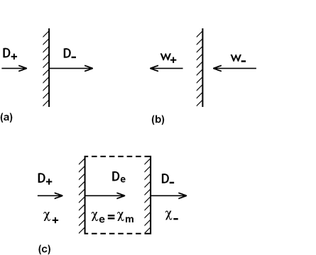
Figure 1: (a): The shock wave [shaded] propagates at velocity $D_{-}$, the flow behind it acquires velocity $D_{+}$. (b): The shock velocities $w_{+}$ and $w_{-}$ are determined in the co-moving reference frame. (c): The joint shock transition is linking currents $\chi_{-}<0$ and $\chi_{+}>0$.

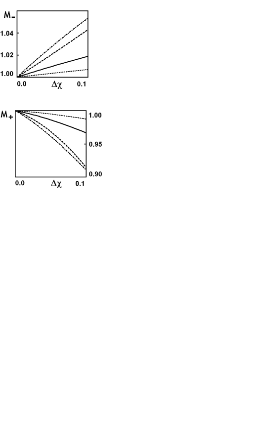
Figure 2: The ratio of shock to sound velocity $M_{-}=w^{2}_{-}/c^{2}_{-}$ (left) and $M_{+}=w^{2}_{+}/c^{2}_{+}$ (right) vs increment $\Delta\chi$ in the magnetic regime of bosonic currents at $m=m_{*}=1$ at initial $\chi_{-}=0.1$ are plotted for four models of EOS: dot - (1), dash - (2), dashdot - (3), solid - (4).

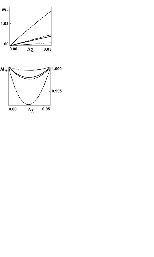
Figure 3: The same plots as in Fig. (2) but in the electric regime of bosonic currents and at initial $\chi_{-}$=-0.05.

References

- [1] T. W. B. Kibble, Phys. Rep. 67, 183 (1980).
- [2] A. Vilenkin, Phys. Rep. 121, 263 (1985).
- [3] V. Berezinsky, B. Hnatyk, and A. Vilenkin Phys. Rev. D 64, 043004 (2001). arXiv:astro-ph/0102366
- [4] F. Ferrer and T. Vachaspati, Int. J. Mod. Phys. D 16, 2399 (2007). arXiv:astro-ph/0608168
- [5] E. Witten, Nucl. Phys. B 249, 557 (1985).
- [6] C. Ringeval, Phys.Rev. D 63 063508 (2001). arXiv:hep-ph/0007015
- [7] N.K. Neilsen and P. Olsen, Nucl. Phys. B 291, 829 (1987).
- [8] D.N. Spergel, T. Piran, and J. Goodman, Nucl. Phys. B 291, 847 (1987).
- [9] E. Copeland, M. Hindmarsh, and N. Turok, Phys. Rev. Lett. 58, 1910 (1987).
- [10] B. Carter, Ann. Phys. (Leipzig) 9, 247 (2000). arXiv:hep-th/0002162
- [11] B. Carter and P. Peter, Phys. Rev. D 52, R1744 (1995). arXiv:hep-ph/9411425
- [12] M. Lilley, P. Peter, and X. Martin, Phys. Rev. D 79, 103514 (2009). arXiv:0903.4328
- [13] B. Hartmann and B. Carter, Phys.Rev. D 77, 103516 (2008). arXiv:0803.0266
- [14] R. L. Davis and E. P. S. Shellard, Nucl. Phys. B 323, 209 (1989).
- [15] Y. Lemperiere and E. P. S. Shellard, Phys.Rev.Lett. 91, 141601 (2003). arXiv:hep-ph/0305156
- [16] B. Carter, Phys. Lett. B 228, 466 (1989).
- [17] X. Martin and P. Peter, Phys. Rev. D 61, 043510 (2000).
- [18] A. Cordero-Cid, X. Martin, and P. Peter, Phys.Rev. D 65, 083522 (2002). arXiv:hep-ph/0201097
- [19] G. Vlasov, Discontinuities on strings, arXiv:hep-th/9905040
- [20] R.A. Battye and P. M. Sutcliffe, Nucl. Phys. B 805, 287 (2008). arXiv:0806.2212
- [21] A. M. Anile, Relativistic fluids and magneto-fluids: with applications in astrophysics and plasma physics (CUP, Cambridge, 1989), p. 61, p. 215.
- [22] A.H. Taub, Ann. Rev. Fluid Mech. 10, 301 (1978).
- [23] L. D. Landau and E. M. Lifshitz, Fluid mechanics, 2nd ed. (Pergamon, Oxford, 1987), p. 331.
- [24] E. Trojan and G.V. Vlasov, Shock waves in superconducting cosmic strings: instability to extrinsic perturbations, arXiv:1103.0673. E. Troyan and Yu.V. Vlasov, Zh.Eksp.Teor.Fiz. (Sov. JETP) 140, 66 (2011).