Ornstein-Uhlenbeck type processes
with heavy distribution tails

Abstract

We consider a transformed Ornstein-Uhlenbeck process model that can be a good candidate for modelling real-life processes characterized by a combination of time-reverting behaviour with heavy distribution tails. We begin with presenting the results of an exploratory statistical analysis of the log prices of a major Australian public company, demonstrating several key features typical of such time series. Motivated by these findings, we suggest a simple transformed Ornstein-Uhlenbeck process model and analyze its properties showing that the model is capable of replicating our empirical findings. We also discuss three different estimators for the drift coefficient in the underlying (unobservable) Ornstein-Uhlenbeck process which is the key descriptor of dependence in the process.

Keywords: Ornstein-Uhlenbeck process, heavy tails, regular variation, rank correlation, Gauss copula, log returns modelling.

AMS 2010 Subject Classification: 62M05; 60J70, 60J60, 62M10.

1 Introduction

There exist a large number of mathematical models designed to reproduce the dynamics of financial data time series and aimed at capturing the key features of their behaviour, one of the most important of them being heavy distribution tails. A recent monographic reference presenting an up-to-date overview of the field is [2], two further monographic references devoted specifically to various aspects of using heavy-tailed distributions being [23, 1]. Despite the abundance of (sometimes rather sophisticated) such models, one cannot claim that there is single widely accepted satisfactory model (or even class of models) for the behaviour of the log prices of traded financial assets. Among the main reasons for that is the ever-changing economical environment that must have substantial effect on the dynamics of the financial time series and hence keeps making the already verified and fitted models obsolete. Furthermore, different uses (which may include options pricing and/or forecasting, at different time scales) of the models stipulate different requirements on their structure and properties, which means there can hardly be a single answer to all the requests. Hence the continuing interest in considering alternative mathematical models that may be successfully used to either get insights in the nature of the log price dynamics or even solve some practical applied problems.

The present note may be considered as a follow-up to a relatively recent paper [11] which analysed a class of rather simple diffusion models for the log prices. The class consists of transformed Ornstein-Uhlenbeck (OU) processes of the form $Y_{t}=h(X_{t}),$ where $h$ is a smooth enough strictly increasing function,

$$dX_{t}=-\alpha X_{t}dt+\tau dW_{t},\qquad t\geq 0,$$ (1)

$W_{t}$ is the standard Wiener process, and $\alpha,\tau>0$ are constants. Clearly, both transition probabilities and stationary distribution are readily available for the process $Y_{t}$, and it was shown in [11] that this class of models (i) allows a closed-form expression for the likelihood function of discrete time observations, (ii) allows the possibility of heavy-tailed observations and (iii) allows the analysis of the tails of the increments. The paper also discussed fitting the model to the log share prices, via approximating by it the hyperbolic diffusion process considered in [4], where the latter model was found to possesses a number of properties encountered in empirical studies of stock prices and was “rather successfully fitted to two different (Danish) stock price data sets”.

However, despite one of the listed in [11] motivations for considering the class being the need to be able to model heavy tailed data, the paper only goes as far as to show (Proposition 2) how to choose $h$ to obtain tail behavior of the form

$$\mathbb{P}(Y_{t}>x)=x^{c}\exp(-ax^{\delta}+b)(1+O(x^{-1})),\qquad x\to\infty,$$

with $\delta\in[1,2],$ $a>0$ and $b,c\in\mathbb{R}$, while Theorem 3 of the paper gives conditions on $h$ under which the transition density will have exponential decay at infinity. This kind of tails can hardly be classified as being heavy. In fact, as it is well-known and will be confirmed in our Section 2 below, one often deals with a power function tail decay for real-life data sets.

The main objectives of the present paper include eliciting conditions on $h$ under which the distribution tails (for the stationary law of $h(X_{t})$, the distributions of the increments $h(X_{t})-h(X_{s})$ and the transition probabilities) for the process $Y_{t}=h(X_{t})$ will have regularly varying behaviour at infinity thus agreeing with empirical observations, and showing that the dependence structure of such a model is also consistent with a typical Australian stock log price behaviour. We used BHP Billiton Ltd prices from 2003–2010 for illustration purposes, but obtained similar results when doing our calculations for several other major companies, both from mining and other sectors of the economy as well, that are listed on the Australian Securities Exchange (ASX), including the ANZ Banking Group Ltd and TOLL Holdings Ltd.

Further arguments in favour of the proposed simple model include the fact that there is good Gaussian fit for the empirical copulas of the process’ values, and the observation that the parameter $\alpha$ characterising the dependence structure of the process can be easily estimated using rank correlations techniques, and that these estimates computed from the time series increments for different time lags agree with each other.

One of the important aspects of mathematical modelling of time series is the choice of the time scale which the modelling will be aimed at. Firstly, the dynamics at different scales can be different, as the key driving factors at these scales may be different — and changing because of changing environment, as it may be happening with the small scale picture over the last years, due to the wide spread of fast algorithmic trading. Secondly, capturing the detail of the small-scale behaviour of prices can be of little help if one is interested in medium or long-term modelling. In our study, we are mostly interested in medium-term modelling, for daily data with time horizons of the order of $10-50$ days. The empirical data we used seem to confirm the appropriateness of the suggested model: even though some of its parameters may be changing with time, it appears that its structure remains consistent with observations.

For further reading and references concerning using OU processes for modelling of financial time series, the interested reader is referred to [19].

The paper is organised as follows. In Section 2 we present the results of an exploratory analysis of the BHP Billiton Ltd log prices time series, to elicit the key features that successful candidate models (for time horizons around 10 days) must possess (tail behaviour, dependence structure). Section 3 presents a theoretical analysis of the model $Y_{t}=h(X_{t})$, $\{X_{t}\}$ following (1), demonstrating conditions on $h$ that lead to regularly varying distribution tail behaviour and also showing that the process’ dependence structure (in terms of rank correlations) is consistent with the real life data properties discussed in Section 2. Section 4 contains a number of comments (mostly concerned with the estimation of $\alpha$) on fitting the suggested model to data. Section 5 presents the proofs of the theorems formulated in the paper.

2 Distributional properties of log returns

A lot of work has been done on studying the distributional properties of the stock (log) price time series, and we refer the interested reader to [2, 1, 23, 9] and the numerous references therein for illuminating discussions of the past findings. However, for the purposes of this research, we decided to do new statistical analysis of a single stock price time series, with a view of looking at the aspects of the empirical data set that can help us clarify the suitability of the transformed OU process model. In this section, we use the time series of daily (closing) prices $S_{t}$ for BHP Billiton Ltd stock as quoted by the ASX, $t=0,1,\ldots,N=2061,$ the day $t=0$ being 1 January 2003, $t=N$ corresponding to 17 December 2010, to elicit the typical distributional properties of the log prices $Z_{t}:=\ln S_{t}$. As we pointed out earlier, we did the same calculations for the stock prices of several other major Australian companies from different sectors of economy (e.g. ANZ Banking Group Ltd and TOLL Holdings Ltd), which yielded quite similar results, so it appears that the data used in this section may be deemed to be typical.

All the data analysis and graphics were done in Matlab.

2.1 The tail behaviour

The usual starting point in data analysis of this kind is to make normal Q-Q-plots. Since we are interested in a dynamic model for the data, we do that for the increments

$$\Delta_{\delta}Z_{t}:=Z_{t}-Z_{t-\delta},\qquad t=\delta,\delta+1,\ldots,N,$$

for different values of $\delta$. Clearly, $\Delta_{\delta}Z_{t}$ is the log return of the stock over a period of time of length $\delta$ ending at time $t$. A typical result is shown in Fig. 1 displaying the plot for $\delta=20$: there is a very good straight line fit in the central part (representing more than 95% of all data, so that the bulk “middle part” of the distribution looks pretty much normal), and then in the end regions there are clear deviations from the straight line indicating the presence of heavy tails. Different time lag values in the range up to $\delta=100$ return rather similar pictures.

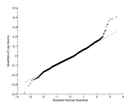
Figure 1: The normal Q-Q plot for the 20 days log-returns $\{\Delta_{20}Z_{t}\}$.

To elicit the character of the tail behaviour of the empirical distributions, one can use the log-log plots of their tails. Figure 2 displays the natural logarithms of the empirical distributions’ left and right tails for the log returns $\{\Delta_{\delta}Z_{t}\}$ against the logs of the data values, for four different time lag values: $\delta=1,5,10$ and 20. The key common features of the plots are: a nice parabolic shape in the “middle region” (which indicates a good normal fit in that region), and then a very good straight line fit for the “remote regions” (comprising about 5% of all data) in all the cases, indicating the power decay of the distributions. An interesting observation is that, for each of the right tails, the slope of the fitting straight line (and hence the index of the approximating power function) is one and the same, for all time lag values.

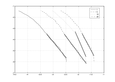
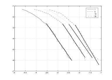
Figure 2: The log-log plots of the empirical distributions’ tails of the BHP stock price log returns for time periods of $\delta=1,5,10,20$ (days). The left (right) pane presents the plots for the left (right, resp.) tails. Straight lines are fitted in each case using the mean squares (the total number of observations from these regions comprise about 5% of all data).

The numerical (absolute) values $\tilde{\beta}_{\pm}(\delta)$ of the slope coefficients of the fitted straight lines for different values of $\delta$ are given in Table 1 (the subscripts $+/-$ correspond to the right/left tails). The table also shows the values of the Hill estimators $\hat{\beta}_{\pm,\{p\}}(\delta)$ for the exponents of the power functions specifying the tail decay rate [10]. Recall that, under the assumption that the right tail of the theoretical distribution of the data $V_{1},\ldots,V_{n}$ with order statistics $V_{1,n}\geq\cdots\geq V_{n,n}$ has a regularly varying form $x^{-\beta_{+}}L(x),$ $L(x)$ being a slowly varying function as $x\to\infty$, the Hill estimator $\hat{\beta}_{+,\{p\}}$ of $\beta_{+}$ is computed according to

$$\frac{1}{\hat{\beta}_{+,\{p\}}}=\frac{1}{k-1}\sum\limits_{i=1}^{k-1}\ln\frac{V_{i,n}}{V_{k,n}},\qquad p=100\,\frac{k}{n}.$$

Note that the estimator was shown to be consistent (as $n\to\infty$, $p\to 0$) for observations forming a strongly mixing sequence [25].

Observe that the estimates obtained by both methods are generally in good agreement, especially for the right tail which appears to be “heavier”. Note that for that tail the values of the estimates for the regular variation index remain roughly the same for all $\delta$ values considered.

	$\delta$	1	5	10	20
Estimators	$\tilde{\beta}_{-}(\delta)\vphantom{\displaystyle\sum}$	2.75	3.28	5.29	4.29
for the	$\hat{\beta}_{-,\{2\}}(\delta)\vphantom{\displaystyle\sum}$	2.88	2.91	5.93	4.09
left tail:	$\hat{\beta}_{-,\{5\}}(\delta)\vphantom{\displaystyle\sum}$	2.80	3.42	3.78	4.53
Estimators	$\tilde{\beta}_{+}(\delta)\vphantom{\displaystyle\sum}$	2.91	3.00	2.87	3.37
for the	$\hat{\beta}_{+,\{2\}}(\delta)\vphantom{\displaystyle\sum}$	3.05	3.47	3.13	3.55
right tail:	$\hat{\beta}_{+,\{5\}}(\delta)\vphantom{\displaystyle\sum}$	2.94	3.11	2.85	3.24

Table 1: Estimates for the exponents of the power functions describing the empirical distribution tail decay for log returns over periods of different lengths $\delta$. Here $\tilde{\beta}_{\pm}$ are obtained as the slope coefficients of the fitted straight lines in Fig. 2, while $\hat{\beta}_{\pm,\{p\}}$ are Hill estimators based on the left-most/right-most $p$% of the data.

2.2 Rank correlations

Now we will turn to analysing the dependence structure of our time series. The standard approach for such a task is based on working with linear correlation coefficients. However, as we saw in Section 2.1, we are dealing here with heavy-tailed data for which using linear correlations may be unwise. For that reason, and also because our intention is to use for modelling purposes a transformation of a Gaussian process with a simple dependence structure, we will prefer to analyse rank correlation coefficients in this section (as they are invariant under strictly increasing transformations and thus may be useful for doing statistical inference for the underlying unobservable process).

As is well known, the values of the two most popular rank correlation measures, Kendall’s tau and Spearman’s rho, are quite close to each other (which was also confirmed by the data we deal with in this section). Because computing the latter requires less computational effort, we chose to work with Spearman’s rho.

Recall (see e.g. [18], pp. 207, 229) that the theoretical value of Spearman’s rank correlation coefficient $\rho_{S}$ for a pair of random variables $U,V$ is defined by

$$\rho_{S}(U,V)=\rho\left(F_{U}(U),F_{V}(V)\right),$$ (2)

where $F_{U}$ and $F_{V}$ are the (marginal) distribution functions of $U$ and $V$, resp., and $\rho$ is the linear correlation. The standard estimator of $\rho_{S}(U,V)$ from a sample $(U_{j},V_{j}),$ $j=1,\ldots,n,$ is calculated using the ranks of the variables within the respective univariate samples as

$$\hat{\rho}_{S}:=\frac{12}{n(n^{2}-1)}\sum\limits_{j=1}^{n}\left(\textrm{rank}(U_{j})-\frac{{n+1}}{2}\right)\left(\textrm{rank}(V_{j})-\frac{n+1}{2}\right).$$ (3)

It is clear that calculating rank correlations for the whole sample of daily data over the eight year long period, without careful detrending and possibly some further data pre-processing, would hardly be meaningful. Furthermore, as we pointed out earlier, we would be most interested in modelling the price processes over medium-term time intervals (about 100 days long), over which one can expect data to follow a reasonably stationary process. And indeed, computing correlations for data from time intervals of such lengths leads to rather stable results. A typical representative is depicted in Fig. 3, showing Spearman’s rho values for the data consisting of the pairs $(Z_{t},Z_{t+k})$, $t=0,1,\ldots,200-k,$ for values $k=1,\ldots,35$. One can observe that the plotted line looks pretty much like an exponential curve, of the form $e^{-ck}$, a behaviour typical of autoregressive processes of the first order (or OU processes in continuous time).

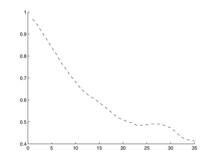
Figure 3: Spearman’s rho for $(Z_{t},Z_{t+k})$, $k=1,\ldots,35$, from the first 200 data points.

For the increments of the time series values, i.e. the log returns over time periods of a fixed length $\delta$, the picture is even more interesting. Following our general approach, here we will pool data from the whole eight year long period of observations, as the influence of the possible (slow) trend present in the time series of the values of the increments of $Z_{t}$ over relatively short lags would be quite small. Fig. 4 shows three plots of Spearman’s rho’s values calculated for the data consisting of the pairs $(\Delta_{\delta}Z_{t},\Delta_{\delta}Z_{t+k}),$ $t=\delta,\delta+1,\ldots,N-k,$ that are plotted for $k=1,2,\ldots,100,$ for the values of $\delta$ equal to 20, 40 and 60.

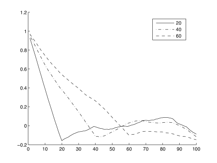
Figure 4: The plots of Spearman’s rhos for the pairs of log returns $(\Delta_{\delta}Z_{t},\Delta_{\delta}Z_{t+k}),$ $t=\delta,\delta+1,\ldots,N-k,$ over time periods of $\delta=20,40$ and 60 days, plotted for $k=1,2,\ldots,100.$

A remarkable common feature of these plots is that they decay in an almost linear way for lag values $k$ from 1 to $\delta$, attaining (small) negative values at the minimum points, and then start slowly growing.

2.3 Copulas

To further analyse the dependence structure of our data, we turn to copulas. One standard way of graphical representation of empirical copulas is to make scatterplots of the pseudo-sample obtained by transforming the components of the sample points using the marginal empirical distribution functions (see e.g. p. 232 in [18]).

We will begin with considering the original data set $\{Z_{t}\}$. To avoid the interference of the possible long-term trend, first we process the original data from blocks of length 100. We consider $20$ subsamples

$$\{(U_{k,j},V_{k,j}):=(Z_{t_{k}+j},Z_{t_{k}+j+5}),\ j=0,1,\ldots,94\},\quad\mbox{\rm where $t_{k}=100k,$ $k=0,1,\ldots,19$},$$

and for each of them produce a sub-pseudosample given by

$$(\hat{U}_{k,j},\hat{V}_{k,j})=\left(\frac{\textrm{rank}(U_{k,j})}{96},\frac{\textrm{rank}(V_{k,j})}{96}\right),\qquad j=0,\ldots,94,$$

where $\textrm{rank}(U_{k,j})$ is the rank of $U_{k,j}$ in the $k$th subsample $U_{k,0},U_{k,1},\ldots,U_{k,94}$, and likewise for $\textrm{rank}(V_{k,j})$. The aggregate pseudosample is then obtained as the union of these 20 sub-pseudosamples and is depicted on the left pane in Fig. 5.

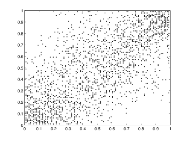
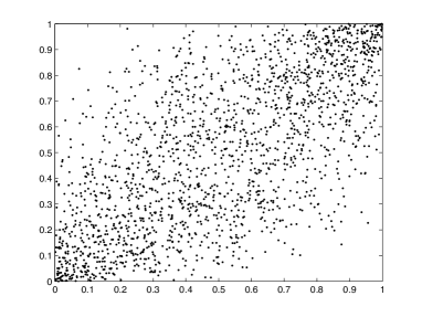
Figure 5: The aggregate scatterplot for the pseudosamples obtained from the data $(Z_{t},Z_{t+5})$ (left pane) and the scatterplot of $N$ simulated points from the Gauss copula $C_{\rho}^{\rm Ga}$ with $\rho=0.693$ obtained from the estimate of Spearman’s rho.

Next to that scatterplot representing the dependence structure for the log prices at lag five, we put the scatterplot of $N$ points simulated from the Gauss copula

$$C_{\rho}^{\rm Ga}(u_{1},u_{2})=\int_{-\infty}^{\Phi^{-1}(u_{1})}\int_{-\infty}^{\Phi^{-1}(u_{2})}\exp\left\{-\frac{x_{1}^{2}-2\rho x_{1}x_{2}+x_{2}^{2}}{2(1-\rho^{2})}\right\}\frac{dx_{1}dx_{2}}{2\pi(1-\rho^{2})^{1/2}},$$ (4)

$\Phi$ being the standard normal distribution function and $\Phi^{-1}$ its inverse, with the parameter $\rho$ value obtained from our estimate for Spearman’s rho. Recall that, for any bivariate random vector $(X_{1},X_{2})$ following a meta-Gaussian distribution with copula (4), one has

$$\rho_{S}(X_{1},X_{2})=\frac{6}{\pi}\arcsin\frac{\rho}{2}$$ (5)

(see e.g. Theorem 5.36 in [18]), so that we can use the estimate $\hat{\rho}=2\sin(\pi\hat{\rho}_{S}/6)$ for $\rho$. In the case of the data set $(Z_{t},Z_{t+5})$, this leads to $\hat{\rho}=0.693.$

No localisation of data followed by the subsequent aggregation is needed for the increments of the original time series values. Figure 6 presents the scatterplot of the pseudosample constructed from the data set $\{(\Delta_{20}Z_{t},\Delta_{20}Z_{t+5}),\,t=20,21,\ldots,N-5\}$, alongside with the scatterplot of a sample simulated from the Gauss copula with the parameter value $\rho=0.695$ (also estimated via (5) from the respective Spearman’s rho).

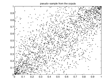
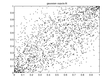
Figure 6: The scatterplot for the pseudosample obtained from the data $(\Delta_{20}Z_{t},\Delta_{20}Z_{t+5})$ (left pane) and the scatterplot of $N$ simulated points from the Gauss copula $C_{\rho}^{\rm Ga}$ with $\rho=0.695$ obtained from the estimate of Spearman’s rho.

We can see that, in both cases, there is a reasonable agreement of the empirical data with the fitted Gauss copulas. To confirm this observation numerically, we used a recently suggested method for calculating approximate $P$-values for testing the goodness-of-fit by parametric copula families [15, 16]. As the method is valid for i.i.d. samples, to use it in our situation we first had to weaken the dependence between sample points by “rarefying” the data. We applied the test to samples obtained by taking each 10th pair of log-returns over two time intervals of length $\delta=1,5,10$ and $20$ days, one shifted by 5 days relative to the other, thus dealing with four bivariate samples each consisting of 206 points of the form $(\Delta_{\delta}Z_{t},\Delta_{\delta}Z_{t+5})$, $t=10,20,30,\ldots,2060.$ The method uses Monte Carlo techniques, and based on 100 simulations from the respective Gauss copulas for each of the $\delta$ values considered, we obtained the following $P$-values: 0.675 ($\delta=1$); 0.332 ($\delta=5$); 0.214 ($\delta=10$); 0.433 ($\delta=20$); so that the Gauss copula hypothesis was not to be rejected.

In conclusion of this section, we summarise its key findings that will be referred to in Section 3:

1. The log returns $\Delta_{\delta}Z_{t}$ over periods of $\delta$ days have distributions of which the “central parts” (about 95% of all data) are very well fitted by the respective parts of normal distributions.

2. The empirical distributions of the log returns $\Delta_{\delta}Z_{t}$ have power tails, with the exponent of the power function (roughly) independent of the lag $\delta$.

3. Spearman’s rho for $(Z_{t},Z_{t+k})$ decays as an exponential function of $k$.

4. As a function of $k$, Spearman’s rho for $(\Delta_{\delta}Z_{t},\Delta_{\delta}Z_{t+k})$ behaves in the fashion presented in Fig. 4.

5. For fixed $k$ and $\delta$, the empirical copulas for both $(Z_{t},Z_{t+k})$ and $(\Delta_{\delta}Z_{t},\Delta_{\delta}Z_{t+k})$ agree with the respective Gauss copulas $C_{\rho}^{\rm Ga}$, with the parameter $\rho$ estimated from the calculated values of Spearman’s rho for the samples. We illustrated that for $k=5$, $\delta=20$, and gave approximate $P$-values for a goodness-of-fit test for Gauss copulas for $(\Delta_{\delta}Z_{t},\Delta_{\delta}Z_{t+k})$ with $k=5$ and $\delta=1,5,10$ and 20, but the situation is similar for other values of the quantities as well.

3 The model and its key properties

In this section, we present a formal description of our simple model suggested by the findings [F₁]–[F₅] and demonstrate that it does have properties consistent with these empirical facts.

Let $\{X_{t}\}$ be a stationary OU process driven by the stochastic differential equation (1). It is well known that $\{X_{t}\}$ is a Gaussian process, with $X_{t}\sim N(0,\sigma^{2})$, where $\sigma^{2}=\tau^{2}/(2\alpha)$. Furthermore, for $0\leq s\leq t$, the conditional distribution of $X_{t}$ given $X_{s}=x$ is normal with mean and variance given by $m_{t-s}(x)$ and $\sigma^{2}_{t-s}$, respectively, where we used notation

$$m_{u}(z):=ze^{-\alpha u},\qquad\sigma^{2}_{u}:=\frac{\tau^{2}}{2\alpha}\,(1-e^{-2\alpha u}),$$

so that the (linear) correlation function of the process has the form

$$\rho(X_{s},X_{t})=e^{-\alpha|t-s|}.$$ (6)

For a strictly increasing continuous mapping $h:\mathbb{R}\to\mathbb{R}$, consider the process

$$Y_{t}:=h(X_{t}),\qquad t\geq 0.$$

It is obvious that $\{Y_{t}\}$ is also a stationary Markov process and, moreover, that if $h$ is twice continuously differentiable then $\{Y_{t}\}$ will be a diffusion process as well. Observe that all finite-dimensional distributions of $\{Y_{t}\}$ are meta-Gaussian: for any $0\leq t_{1}<t_{2}<\cdots<t_{n}$, the vector $(Y_{t_{1}},\ldots,Y_{t_{n}})$ has a Gauss copula with the correlation matrix $\left(\rho_{ij}=e^{-\alpha|t_{i}-t_{j}|}\right)_{i,j\leq n}$ and identical univariate marginal d.f.’s all equal to $F(y):=\mathbb{P}(Y_{t}\leq y)=\Phi(h^{-1}(y)/\sigma)$, $\Phi$ being the standard normal d.f.

Our first objective will be to determine conditions on $h$ under which one or both of the distribution tails of $Y_{t}$ is/are of regular variation, so that for the d.f. $F$ of $Y_{t}$ one has

$$\overline{F}(y):=1 -F(y)=y^{-\beta_{+}}L_{+}(y)$$ (7)

and/or

$$F(-y) =y^{-\beta_{-}}L_{-}(y),$$ (8)

where $\beta_{\pm}>0$ and $L_{\pm}$ are functions slowly varying as $y\to\infty.$

To this end, we will introduce two conditions [A₊] and [A_-] as follows:

[A_±] For some constant $b_{\pm}>0$ and differentiable function $f_{\pm}(x)$, one has

$$h(x)=\pm\exp\{b_{\pm}x^{2}+f_{\pm}(x)+o(1)\}\quad\mbox{\em with \ $f^{\prime}_{\pm}(x)=o(x)$ \ as \ $x\to\pm\infty$}.$$ (9)

Now we can state the following key result on the tail behaviour.

Theorem 1.

The following assertions hold true.

(i) Under condition [A₊], the stationary distribution $F$ of $Y_{t}$ has a right tail of the form (7) with $\beta_{+}=1/(2b_{+}\sigma^{2})=\alpha/(b_{+}\tau^{2})$.

(ii) Similarly, under condition [A_-] the left tail of $F$ is of the form (8) with $\beta_{-}=1/(2b_{-}\sigma^{2})=\alpha/(b_{-}\tau^{2})$.

(iii) Under condition [A₊], the right tail of the transition distribution function $F_{s,t}(y_{s},y_{t}):=\mathbb{P}(Y_{t}\leq y_{t}\,|\,Y_{s}=y_{s}),$ $0\leq s<t,$ is regularly varying of index

$$-\beta_{+,t-s}:=-\frac{1}{2b_{+}\sigma_{t-s}^{2}}=-\frac{\alpha}{b_{+}\tau^{2}(1-e^{-2\alpha(t-s)})}<-\beta_{+}.$$

Under condition [A_-], a symmetric assertion holds for the left tail of the transition distribution, with the regular variation index $-\beta_{-,t-s}:=-(2b_{-}\sigma_{t-s}^{2})^{-1}$.

(iv) If [A₊] is met and $h(-x)=o(h(x))$ as $x\to\infty$, then, for any $0\leq s<t,$ the right tail of the distribution of the increment $Y_{t}-Y_{s}$ in the stationary process has the same regularly varying asymptotic behaviour at infinity as that of $Y_{t}$ from part (i). Similarly, if [A_-] holds and $h(x)=o(h(-x))$ as $x\to\infty$, then the right tail of the increment $Y_{t}-Y_{s}$ in the stationary process has the same regularly varying asymptotic behaviour at infinity as the left tail of $F$ from part (ii).

The proof of the theorem is given in Section 5.

Now suppose that our $h$ is linear in the “middle part”: say, on an interval $I$ such that $\mathbb{P}(X_{t}\in I)\geq 1-\varepsilon/2$ (with a small enough $\varepsilon$), we have

$$h(x)=a+cx,\qquad x\in I,$$

for some constants $a\in\mathbb{R}$, $c>0$, and then outside $I$ the function $h$ has “tail parts” satisfying conditions [A_±]. Then, assuming that the log price time series $\{Z_{t}\}$ is represented by (the values at integer time points $t$ of) the process $\{Y_{t}=h(X_{t})\}$, we will have for the log returns a representation of the form

$$\Delta_{\delta}Z_{t}=h(X_{t})-h(X_{t-\delta})=c(X_{t}-X_{t-\delta})+\xi_{t,\delta},\qquad\mathbb{P}(\xi_{t,\delta}\neq 0)\leq\varepsilon,$$ (10)

since $\{\xi_{t,\delta}\neq 0\}\subset\{X_{t}\not\in I\}\cup\{X_{t-\delta}\not\in I\}.$ Therefore the “central part” of the distribution of $\Delta_{\delta}Z_{t}$ will be very close to that of $c(X_{t}-X_{t-\delta})$, which is clearly normal. This shows that our model is consistent with empirical fact [F₁].

That [F₂] is also reproduced by the model follows from Theorem 1(iv). Here a curious observation is in order. On the one hand, the log-log plots in Fig. 2 display “shifted” parallel straight line segments in the curves corresponding to different values of $\delta$, and such a translation indicates that the tail behaviours of the returns’ distributions for different $\delta$’s differ by constant factors (increasing with $\delta$). On the other hand, Theorem 1(iv) claims that they should have common asymptotics, which seems to be a contradiction. However, large sample simulations of the differences of transformed components of Gaussian vectors demonstrate the same translation of the straight line segments present in the log-log plots of the empirical distribution tails for increments, corresponding to different $\delta$ values, in the “moderately large” deviations zone (in agreement with the empirical observations), which is then followed by a “fusion” of the curves for larger deviation values thus confirming the common asymptotics established in Theorem 1(iv). The proof of the theorem suggests the following explanation for this phenomenon: the established (common) asymptotics are essentially due to the convergence of the conditional probability in the integral on the right-hand side of (21) (or, rather, the conditional probability $\mathbb{P}(Y_{s}<z-y\mid Y_{t}=z)$ in $I_{3}$, see (16)) to one. However, in vicinity of the lower integration limit $(1+\varepsilon)y$ in $I_{3}$ this convergence is slow. In combination with the regular variation of the right tail of the distribution of $Y_{t}$, this results in a “pre-limiting” tail beahaviour differing from that of $\mathbb{P}(Y_{t}>y)$ by a factor depending on $\delta=t-s$ and $y$, which can be small for small $\delta$ (hence the translation of the plots), but which eventually tends to one as $y\to\infty$.

To illustrate the above statement concerning the simulation study, Fig. 7 displays the log-log plots of the empirical distribution tails for three i.i.d. samples (of size $3\times 10^{5}$ each) of the differences $h(\zeta_{2})-h(\zeta_{1})$, where

$$h(x)=2(e^{(3+{\rm sign}\,x)x^{2}/20}-1)\,\mbox{sign}\,x+x,\qquad x\in\mathbb{R},$$ (11)

has the form stipulated in (9), with $b_{+}=0.2$ and $b_{-}=0.1$, and $(\zeta_{1},\zeta_{2})$ have standard normal bivariate distributions with correlations $e^{-a}$, with $a=0.5$ (the left curve), 1 and 1.5 (the right curve), respectively, playing the role of $\alpha\delta$.

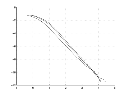
Figure 7: The log-log plots of the empirical distribution tails for simulated differences $h(\zeta_{2})-h(\zeta_{1})$ for i.i.d. standard Gaussian random vectors $(\zeta_{1},\zeta_{2})$ with different correlations (for detailed description, see the text around formula (11)).

That property [F₃] holds for $\{Z_{t}:=h(X_{t})\}$ follows from the exponential form of the correlation function (6), the invariance of Spearman’s rho under strictly increasing transformations (so that $\rho_{S}(h(X_{s}),h(X_{t}))=\rho_{S}(X_{s},X_{t})$) and relation (5) (note that the function of $\rho$ on the RHS of (5) is very close to the identity function on the interval $\rho\in[-1,1]$).

The demonstration of [F₄] is somewhat less straightforward. First we state the following bound of which the proof is given in Section 5. As can be seen from the proof, the bound is rather conservative, and so the result is more qualitative than quantitative in nature: one can expect that, in most cases, the distance between the values of the Spearman’s rhos will be much smaller than the bound given.

Theorem 2.

Let $U$, $V$, $\xi$ and $\eta$ be random variables given on a common probability space and such that $U$, $V$ and the sums

$$U_{1}:=U+\xi,\qquad V_{1}:=V+\eta$$

are all continuously distributed. Then, setting $\mathbb{P}(\xi\neq 0)=:\varepsilon_{1}$ and $\mathbb{P}(\eta\neq 0)=:\varepsilon_{2},$ one has

$$|\rho_{S}(U_{1},V_{1})-\rho_{S}(U,V)|\leq 18(\varepsilon_{1}+\varepsilon_{2})+12\varepsilon_{1}\varepsilon_{2}.$$

From that bound and (10) it follows that

$$\bigl{|}\rho_{S}(\Delta_{\delta}Z_{t},\Delta_{\delta}Z_{t+k})-\rho_{S}(\Delta_{\delta}X_{t},\Delta_{\delta}X_{t+k})\bigr{|}\leq\varepsilon_{0},$$

where $\varepsilon_{0}=36\varepsilon+12\varepsilon^{2}.$ Here $(\Delta_{\delta}X_{t},\Delta_{\delta}X_{t+k})\equiv(X_{t}-X_{t-\delta},X_{t+k}-X_{t+k-\delta})$ has a joint Gaussian distribution, and so in view of the above-stated relationship (5) between $\rho_{S}$ and $\rho$ in the Gaussian case, it remains to evaluate the linear correlation

$$\rho(\Delta_{\delta}X_{t},\Delta_{\delta}X_{t+k})=\frac{\mathbb{E}(X_{t}-X_{t-\delta})(X_{t+k}-X_{t+k-\delta})}{\mbox{\rm Var}(X_{t}-X_{t-\delta})},$$

where we used the stationarity and zero means of $\{X_{t}\}$. Expanding the numerator and employing (6), we obtain, for $k\geq 0$ and $\delta>0$,

$$\mathbb{E}(X_{t}-X_{t-\delta})(X_{t+k} -X_{t+k-\delta})$$

$$=\mathbb{E}X_{t}X_{t+k}-\mathbb{E}X_{t}X_{t+k-\delta}-\mathbb{E}X_{t-\delta}X_{t+k}+\mathbb{E}X_{t-\delta}X_{t+k-\delta}$$

$$=\sigma^{2}\bigl{(}2\rho(X_{t},X_{t+k})-\rho(X_{t},X_{t+k-\delta})-\rho(X_{t},X_{t+k+\delta})\bigr{)}$$

$$=\sigma^{2}\bigl{(}2e^{-\alpha k}-e^{-\alpha|k-\delta|}-e^{-\alpha(k+\delta)}\bigr{)}.$$

As a special case of this where $k=0,$ we have $\mbox{\rm Var}(X_{t}-X_{t-\delta})=2\sigma^{2}(1-e^{-\alpha\delta})$, so that

$$\rho(\Delta_{\delta}X_{t},\Delta_{\delta}X_{t+k})=\frac{2e^{-\alpha k}-e^{-\alpha|k-\delta|}-e^{-\alpha(k+\delta)}}{2(1-e^{-\alpha\delta})}.$$

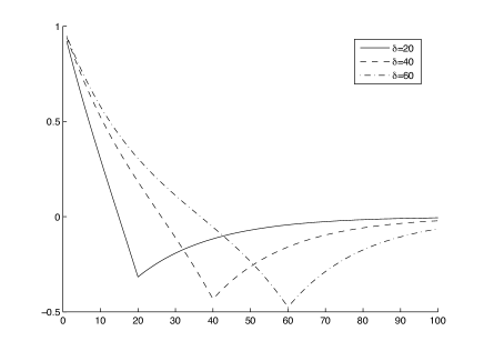
Figure 8: The plots of the correlation functions $\rho(\Delta_{\delta}X_{t},\Delta_{\delta}X_{t+k})$ in the case $\alpha=0.05,$ for $\delta=20,40$ and 60 days, plotted for $k\leq 100$ (cf. Fig. 4).

The plots of this function of $k$ for three different values of $\delta$ are presented in Fig. 8. They demonstrate virtually the same behaviour as the empirical Spearman’s rhos shown in Fig. 4, thus confirming that our model has property [F₄].

Concerning [F₅], we immediately see that, for our model $Y_{t}=h(X_{t})$, the vector $(Y_{t},Y_{t+k})$ clearly has a Gauss copula. As it was the case when dealing with [F₄], showing that the copula for the vector of increments $(\Delta_{\delta}Y_{t},\Delta_{\delta}Y_{t+k})$ will be close to a Gauss one, provided that the value of $\varepsilon$ in (10) is small, is a more sophisticated task. However, that can be easily done adapting the proof of Theorem 2 and its extension to the case of bivariate distribution functions. This is a straightforward technical exercise that we leave to the interested reader.

Remark 1.

A possible relatively simple modelling approach alternative to ours would be to use, instead of (1), a stochastic driver of the form

$$dX_{t}=-\alpha X_{t}dt+dL_{t},$$ (12)

where $\{L_{t}\}$ is a suitably chosen Lévy process. In particular, Theorem 3.2 in [9] establishes the following result: Let $\mu\in\mathbb{R}$ and $\nu,\lambda>0$ be arbitrary,

$$K_{\nu}(x) =\frac{1}{2}\int_{0}^{\infty}y^{\nu-1}\exp\left\{-\frac{x}{2}\left(y+y^{-1}\right)\right\}dy$$

$$\equiv\frac{1}{2}\int_{-\infty}^{\infty}\exp\left\{\nu u-x\cosh u\right\}du,\qquad x>0,$$

be the modified Bessel function of the third kind, and $\{L_{t}\}_{t\geq 0}$ be a Lévy process with cumulant function

$$\ln\mathbb{E}e^{iuL_{1}}=iu\mu-\lambda|u|\frac{K_{\nu/2-1}(\lambda|u|)}{K_{\nu/2}(\lambda|u|)},\qquad u\in\mathbb{R}\setminus\{0\}.$$

Then the stochastic differential OU type equation (12) has a weak strictly stationary solution satisfying

$$X_{t}=e^{-\alpha t}X_{0}+e^{-\alpha t}\int_{0}^{t}e^{\alpha s}dL_{s}$$

and such that $X_{t}$ has marginal $t$-distribution $T(\nu,\lambda,\mu)$ with density

$$\frac{c(\nu,\lambda)}{[1+((x-\mu)/\lambda)^{2}]^{(\nu+1)/2}},\qquad x\in\mathbb{R},$$

where $c(\nu,\lambda)=(\lambda{\rm B}(\nu/2,1/2))^{-1}$, ${\rm B}(\cdot,\cdot)$ being the beta function. Moreover, if $\nu>1$ then $\mathbb{E}X_{t}=\mu$, and if $\nu>2$ then $\mbox{\rm corr}\,(X_{t+\tau},X_{t})=e^{-\alpha|\tau|}$.

As the resulting process $\{X_{t}\}$ will already have power function decay of the distribution tails, it might be possible to use that process for modelling the financial data of interest, without transforming it (although some transformation might still be needed, due to the symmetry of $t$ distributions). The advantage of using a transformed OU model of the type dealt with in the present paper is that it is more flexible as its temporal dependence structure can be decoupled from its distribution tail properties.

4 Further comments on model fitting

First we observe that, without loss of generality, one can always put $\tau=1$ in (1): indeed, we clearly have $Y_{t}=\tilde{h}(\tilde{X}_{t})$ with $\tilde{h}(x):=h(\tau x)$ and $\tilde{X}_{t}:=\tau^{-1}X_{t}$ satisfying

$$d\tilde{X}_{t}=-\alpha\tilde{X}_{t}dt+dW_{t},\qquad t\geq 0.$$

So in the “driver” component (1) of the model, one only needs to estimate $\alpha$, and it is this task that will be discussed in the present section.

Concerning the estimation of the function $h$, we will only point out that, in view of its specific form dictated by Theorem 1, a parametric approach would be most natural. One possible simple parametric class of functions consists of candidates of the following spline type:

$$h(x)=-a_{1}e^{b_{-}x^{2}}{\bf 1}(x\leq x_{1})+(a_{2}+a_{3}x){\bf 1}(x_{1}<x\leq x_{2})+a_{4}e^{b_{+}x^{2}}{\bf 1}(x>x_{2}),$$

where ${\bf 1}(\cdot)$ denotes the indicator function, the bounds $x_{i}$ can be estimated as the end points of the “central part” of the distribution well approximated by a normal one, $a_{2}$ and $a_{3}>0$ can be estimated from that “central part” (i.e. from a truncated sample), parameters $b_{\pm}>0$ can be estimated using estimates for the tail regular variation indices (e.g. Hill estimators) and the assertions of Theorem 1 (note that, to use them, one has to estimate $\alpha$ first), and $a_{1}$ and $a_{4}$ can be chosen to make the function $h$ continuous. Alternative parametric families may be more adequate.

Suppose that the process $\{Y_{t},t\in[0,T]\}$ is observed at times $t_{k}=k\epsilon$, $k=0,\ldots,n$, where $n+1$ is the total number of observations. Without loss of generality, we can always assume that $\epsilon=1$.

4.1 An estimator based on rank correlations

Since Spearman’s rho is invariant under strictly increasing transformations of data and $(X_{j},X_{k})$ is Gaussian, we have from (5) that

$$\rho_{S}(Y_{j},Y_{k})=\rho_{S}(X_{j},X_{k})=\frac{6}{\pi}\arcsin\frac{\rho(X_{j},X_{k})}{2}=\frac{6}{\pi}\arcsin\frac{e^{-\alpha|j-k|}}{2},$$

so that

$$\alpha=-\frac{1}{|j-k|}\ln\left(2\sin\left(\frac{\pi}{6}\rho_{S}(Y_{j},Y_{k})\right)\right).$$

Hence one can use the “plug-in” estimators

$$\hat{\alpha}_{k}:=-\frac{1}{k}\ln\left(2\sin\left(\frac{\pi}{6}\hat{\rho}_{S}(Y_{0},Y_{k})\right)\right),\qquad k=1,2,\ldots,$$

where $\hat{\rho}_{S}(Y_{0},Y_{k})$ is calculated according to (3), for the sample of pairs $(Y_{t},Y_{t+k})$. As discussed before, such an estimation would require blocking of data, to reduce the effect of the slow trend component in the time series. Alternatively, one can use Spearman’s rho for the increments of $Y_{t}$ (cf. our discussion following Theorem 2). The values of $\hat{\alpha}_{k}$ for different $k$’s obtained from 50 day log-returns for BHP data are shown in Table 2. Note the stability of the estimates, which confirms the appropriateness of the model (according to which the quantities are estimators of the same value).

$k$	5	10	15	20	25	30
$\hat{\alpha}_{k}$	0.032	0.036	0.036	0.037	0.036	0.038

Table 2: The values of $\hat{\alpha}_{k}$ from 50 day BHP stock log returns, for different values of $k$.

4.2 An alternative estimator

An alternative (but closely related) estimator for $\alpha$ is based on the following simple observation concerning the background OU process, which we will formulate in the form of a theorem (for its proof, see Section 5). Set

$$g(x):=-\ln\left[\sin\left(2\pi(x-1/4)\right)\right],\qquad x\in(1/4,1/2).$$

Theorem 3.

Let

$$\hat{p}_{k}^{0}:=\frac{1}{n-k}\sum\limits_{j=0}^{n-k}\mathbf{1}(X_{j}>0,X_{j+k}>0)$$

be an empirical estimate of $p_{k}:=\mathbb{P}(X_{0}>0,X_{k}>0)$. Then

$$\hat{\alpha}^{0}_{k}:=\frac{g(\hat{p}^{0}_{k})}{k},\qquad k=1,2,\ldots,$$ (13)

are strongly consistent and asymptotically normal $($as $n\to\infty)$ estimators of $\alpha$ with

$${\rm Var}(\hat{\alpha}^{0}_{k})\sim\frac{v^{2}_{k}(g^{\prime}(p_{k}))^{2}}{nk^{2}},$$

where

$$v^{2}_{k}:=p_{k}(1-p_{k})+2\sum\limits_{l=1}^{\infty}\left(\mathbb{P}(X_{k+l}>0,X_{l}>0,X_{k}>0,X_{0}>0)-p_{k}^{2}\right).$$ (14)

Of course, in the context of our problem $\{X_{t}\}$ is unobservable, so we need to replace $\hat{p}^{0}_{k}$ with an estimator for $p_{k}$ from $\{Y_{t}\}$. Denoting by $m$ the median of $F$, we clearly have $\{X_{j}>0\}=\{Y_{j}>m\}$ and so

$$\hat{p}_{k}^{0}=\frac{1}{n-k}\sum\limits_{j=0}^{n-k}\mathbf{1}(Y_{j}>m,Y_{j+k}>m).$$

We still do not know $m$, but one can use instead the empirical median $\hat{m}_{n}(Y)$ of the sample $Y_{0},Y_{1},\ldots,Y_{n}$. It is not hard to verify that $\hat{m}_{n}(Y)\stackrel{{\scriptstyle{\rm a.s.}}}{{\longrightarrow}}m$ as $n\to\infty$, which implies that

$$\hat{p}_{k}:=\frac{1}{n-k}\sum\limits_{j=0}^{n-k}\mathbf{1}(Y_{j}>\hat{m}_{n}(Y),Y_{j+k}>\hat{m}_{n}(Y))\stackrel{{\scriptstyle{\rm a.s.}}}{{\longrightarrow}}p_{k}.$$

Therefore

$$\hat{\alpha}^{\prime}_{k}:=\frac{g(\hat{p}_{k})}{k},\qquad k=1,2,\ldots,$$

will also be strongly consistent estimators of $\alpha$.

The values of $\hat{\alpha}^{\prime}_{k}$ for different $k$’s obtained from 50 day log-returns for BHP data are shown in Table 3.

$k$	5	10	15	20	25	30
$\hat{\alpha}^{\prime}_{k}$	0.027	0.035	0.035	0.032	0.031	0.031

Table 3: The values of $\hat{\alpha}^{\prime}_{k}$ from 50 day BHP stock log returns, for different values of $k$.

Simulations showed that the root mean square errors of the estimators $\hat{p}_{k}$ are smaller than those for $\hat{p}_{k}^{0}$, so that from the viewpoint of the quadratic error minimisation it is better, in a sense, not to know the true value of the median of the stationary distribution $F.$ Figure 9 displays the values of the ratio of the standard error of $\hat{p}_{k}^{0}$ to that of $\hat{p}_{k}$, for $k=20$, calculated from a sample of $10^{4}$ independent discretised trajectories of the OU process on the time interval $[0,T]$, with $T=10^{4}$ and discretisation step $\epsilon=1.$

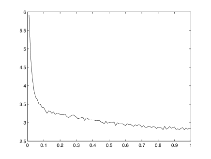
Figure 9: The ratio of the root mean square errors of $\hat{p}_{20}^{0}$ and $\hat{p}_{20}$ as a function of $\alpha$ calculated using crude Monte-Carlo simulations of the respective OU process.

It can be seen from the plot that, as $\alpha$ increases, the value of the ratio appears to decrease to some limiting value. That limiting value should correspond to the case of independent observations $Y_{j}$, $j=0,1,2,\ldots,n$ (or $X_{j}$), in which the ratio can be calculated, as shows Theorem 4 below (its proof is given in Section 5). Unfortunately, we were not able to quantify the effect in the general case, for finite values of $\alpha$, but a plausible “common sense explanation” of it remains the same: the “quality” of the estimators $\hat{p}_{k}^{0}$ and $\hat{p}_{k}$ is basically determined by how often the difference $X_{j}-a$ changes its sign, for $a=0$ and $a=\hat{m}_{n}(X)$, respectively, and in the latter case this occurs more often.

For notational convenience, in Theorem 4 we will consider samples starting from $X_{1}$ (rather than $X_{0}$), so that here we will have

$$\hat{p}_{k}^{0} :=\frac{1}{n-k}\sum\limits_{j=1}^{n-k}\mathbf{1}(X_{j}>0,X_{j+k}>0),$$

$$\hat{p}_{k} :=\frac{1}{n-k}\sum\limits_{j=1}^{n-k}\mathbf{1}(X_{j}>\hat{m}_{n}(X),X_{j+k}>\hat{m}_{n}(X)),$$

$\hat{m}_{n}(X)$ being the sample median for $X_{1},X_{2},\ldots,X_{n}$.

Theorem 4.

Let $X_{1},X_{2},\ldots,X_{n}$ be i.i.d. standard normal random variables and $p_{k}:=\mathbb{P}(X_{j}>0,X_{j+k}>0)$, $k=1,2,\ldots$ Then, for any fixed $k$, $\hat{p}_{k}^{0}$ is an unbiased estimator of $p_{k}=1/4$, $\hat{p}_{k}$ has a bias of $O(n^{-1})$ as $n\to\infty$, and

$${\rm Var\,}(\hat{p}_{k}^{0})=\frac{5}{16n}+O(n^{-2}),\qquad{\rm Var\,}(\hat{p}_{k})=\mathbb{E}(\hat{p}_{k}-p_{k})^{2}+O(n^{-2})=\frac{1}{16n}+O(n^{-2}).$$

4.3 An estimator based on band crossing times

In the two previous subsections we considered estimation of the drift coefficient $\alpha$ of the unobservable OU process $\{X_{t}\}$ from its transformed version $\{Y_{t}=h(X_{t})\}$ which was assumed to be observable. It is interesting to note that one can estimate $\alpha$ even if $\{Y_{t}\}$ is only partially observable itself — namely, if we only know the number of times the process’ trajectory crossed the band between two given levels $A$ and $B$ during a given time interval, provided that we also know the values of the d.f. $F(y)$ of the stationary distribution of $Y_{t}$ at the points $y=A,B$.

For $a,b\in\mathbb{R}$ denote by $T_{a,b}$ the time it takes the OU process $\{X_{t}\}$ driven by (1) with $\tau=1$ to transit from point $b$ to point $a$: slightly abusing notation, one can write

$$T_{a,b}:=\inf\{t>0:X_{t}=a\mid X_{0}=b\}.$$

The density of $T_{a,b}$ has a simple closed-form representation when $a=0$ [26]; in the general case, this is not so (one needs to invert a Laplace transform expressed in terms of parabolic cylinder functions, see e.g. [24]). However, for our purposes it will be enough to know the means of $T_{a,b}$ only, and these are available, see [24].

By the excursion time $T_{(a),b}$ to $a$ from $b$ we will call the time it takes the OU process starting from $b$ to reach the point $a$ and then return back to $b$. Clearly,

$$T_{(a),b}\stackrel{{\scriptstyle d}}{{=}}T_{a,b}+T_{b,a},$$

where the random variables on the right-hand side are assumed to be independent.

Set $a:=h^{-1}(A)$, $b:=h^{-1}(B)$. Since $X_{t}\sim N(0,1/(2\alpha))$ in the stationary regime, one has $\Phi(\sqrt{2\alpha}a)=\mathbb{P}(X_{t}\leq a)=\mathbb{P}(h(X_{t})\leq A)=F(A)$ and likewise $\Phi(\sqrt{2\alpha}b)=F(B)$. Therefore

$$a=\frac{\Phi^{-1}(F(A))}{\sqrt{2\alpha}}=:\frac{a^{*}}{\sqrt{\alpha}},\qquad b=\frac{\Phi^{-1}(F(B))}{\sqrt{2\alpha}}=:\frac{b^{*}}{\sqrt{\alpha}}.$$

The standard scaling argument shows that the process $X^{*}_{t}:=\alpha^{1/2}X_{t/\alpha}$ satisfies (1) with $\alpha=1,$ $\tau=1$ (and another Brownian motion process, namely $W^{*}_{t}=\alpha^{1/2}W_{t/\alpha}$, instead of $W_{t}$). Therefore one has

$$T_{(a),b}\stackrel{{\scriptstyle d}}{{=}}\alpha^{-1}T^{*}_{(a^{*}),b^{*}},$$

where the asterisk indicates that the excursion time on the right hand side is for the process $\{X^{*}_{t}\}$, the distribution of $T^{*}_{(a^{*}),b^{*}}$ being independent of $\alpha$ and having a mean $m_{a^{*},b^{*}}$ which can be computed from $F(A)$ and $F(B)$ using the results of [24].

Now the strong Markov property implies that the subsequent excursions from $b$ to $a$ in $\{X_{t}\}$ (or, equivalently, from $B$ to $A$ in $\{Y_{t}\}$) form an i.i.d. sequence. Therefore, if $N_{A,B}(T)$ denotes the number of times $\{Y_{t}\}$ crosses the band between the levels $A$ and $B$ in a given direction (say, from $B$ to $A$, each such crossing corresponding to an excursion from $B$ to $A$) during the time interval $[0,T]$, the integral renewal theorem asserts that, as $T\to\infty$,

$$\frac{N_{A,B}(T)}{T}\stackrel{{\scriptstyle{\rm a.s.}}}{{\longrightarrow}}\frac{1}{\mathbb{E}T_{(a),b}}=\frac{\alpha}{m_{a^{*},b^{*}}},$$

which leads to another consistent estimator of $\alpha$ given by $\hat{\alpha}^{\prime\prime}:=m_{a^{*},b^{*}}N_{A,B}(T)T^{-1}.$ In conclusion we note that one can evaluate the mean quadratic error of the estimator $\hat{\alpha}^{\prime\prime}$ from the central limit theorem for renewal processes (the variance of $T_{a,b}$ is also available from [24]).

5 Proofs

Proof of Theorem 1.

(i), (ii) As part (ii) is a “mirror reflection” of part (i), we only need to prove the latter (in fact, part (ii) was included in the theorem as a separate assertion only for convenience of referencing to it in part (iv)).

Set $x:=h^{-1}(y).$ Since $X_{t}\sim N(0,\sigma^{2})$, we can use Mills’ ratio for the normal tail and the relation $b_{+}\beta_{+}=1/(2\sigma^{2})$ to write that, as $y\to\infty,$

$$\mathbb{P}(Y_{t}>y) =\mathbb{P}(X_{t}>x)=\frac{\sigma}{x\sqrt{2\pi}}e^{-x^{2}/(2\sigma^{2})}(1+o(1))$$

$$=\frac{\sigma}{x\sqrt{2\pi}}\left(e^{b_{+}x^{2}}\right)^{-\beta_{+}}\left(1+o(1)\right)=\frac{\sigma}{x\sqrt{2\pi}}\,e^{\beta_{+}f_{+}(x)+o(1)}(h(x))^{-\beta_{+}}$$

$$=\frac{\sigma}{\sqrt{2\pi}}\,e^{\beta_{+}f_{+}(x)-\ln x+o(1)}y^{-\beta_{+}}.$$ (15)

It remains to show that $g(y):=e^{f_{0}(x)}$, where $f_{0}(x)=\beta_{+}f_{+}(x)-\ln x$ and $x=h^{-1}(y),$ is a slowly varying function of $y$. To this end, fixing an arbitrary $\lambda>1$ and setting $s:=h^{-1}(\lambda y)-x$, we can write

$$\frac{g(\lambda y)}{g(y)}=\exp\{f_{0}(x+s)-f_{0}(x)\}.$$

Since clearly $f_{0}^{\prime}(x)=o(x)$ as $x\to\infty,$ it now suffices to show that $s=O(1/x)$ .

From the definition of $s$, the mean value theorem and the assumption $f^{\prime}_{+}(x)=o(x),$ we have

$$\lambda =\frac{h(x+s)}{h(x)}=\exp\{2b_{+}xs+b_{+}s^{2}+f_{+}(x+s)-f_{+}(x)+o(1)\}$$

$$=\exp\{2b_{+}xs(1+o(1))+bs^{2}+o(1)\},$$

which immediately implies that $s=O(1/x)$ and hence completes the proof of part (i).

(iii) We will only consider the case where [A₊] holds true. The case of [A_-] is dealt with in the same way.

First observe that, given $Y_{s}=y_{s}$ (or, equivalently, $X_{t}=x_{s}:=h^{-1}(y_{s})$), we can write the increment of the process $\{Y_{t}\}$ on $[s,t]$ as

$$Y_{t}-y_{s}=h(X_{t})-h(x_{s})=h_{1}(X_{t}-m_{t-s}(x_{s}))-h(x_{s}),$$

where, setting for brevity $m:=m_{t-s}(x_{s})$, the function

$$h_{1}(x)=h(x+m)=\exp\{bx^{2}+2bmx+m^{2}+f(x+m)+o(1)\}=:e^{bx^{2}+f_{1}(x)+o(1)}$$

is again of the form (9), with $f_{1}(x):=2bmx+m^{2}+f(x+m)$ clearly satisfying the relation $f_{1}^{\prime}(x)=o(x).$ Since, as we have already recalled, the conditional distribution of $X_{t}-m_{t-s}(x_{s})$ given $X_{t}=x_{s}$ is $N(0,\sigma_{t-s}^{2})$, the proof of (iii) is completed by the same argument as used to demonstrate the first part of the theorem.

(iv) We will prove the first part of the assertion, assuming that [A₊] is met and $h(-x)=o(h(x))$ as $x\to\infty$. The second half will then immediately follow, in view of the observations that $Y_{t}-Y_{s}=-(Y_{s}-Y_{t})$ and $(Y_{s},Y_{t})\stackrel{{\scriptstyle d}}{{=}}(Y_{t},Y_{s})$, the latter being a consequence of the obvious relation $(X_{s},X_{t})\stackrel{{\scriptstyle d}}{{=}}(X_{t},X_{s})$ (for the stationary OU process, of course).

Letting $y\to\infty$ and $\varepsilon=\varepsilon(y)\downarrow 0$ slowly enough (so that, in particular, $\varepsilon y\to\infty$; further conditions on the behaviour of $\varepsilon$ will appear later), we can write

$$\mathbb{P}(Y_{t}-Y_{s}>y) =\int\mathbb{P}(Y_{s}<z-y,\,Y_{t}\in dz)$$

$$=\int_{-\infty}^{(1-\varepsilon)y}+\int_{(1-\varepsilon)y}^{(1+\varepsilon)y}+\int_{(1+\varepsilon)y}^{\infty}=:I_{1}+I_{2}+I_{3}.$$ (16)

First consider

$$I_{1} =\int_{-\infty}^{(1-\varepsilon)y}\mathbb{P}(Y_{s}<z-y,\,Y_{t}\in dz)\leq\int_{-\infty}^{(1-\varepsilon)y}\mathbb{P}(Y_{s}<-\varepsilon y,\,Y_{t}\in dz)$$

$$=\mathbb{P}(Y_{s}<-\varepsilon y,\,Y_{t}\leq(1-\varepsilon)y)\leq\mathbb{P}(Y_{s}<-\varepsilon y)=\mathbb{P}(-h(X_{s})>\varepsilon y).$$ (17)

In the case where $\inf_{x}h(x)>-\infty$ one clearly has $I_{1}=0$ for all large enough $y$. In the alternative case, the function $v(w):=-h^{-1}(-w)$ will be defined for all $w\in\mathbb{R}$ and have the property $v(w)\to\infty$ as $w\to\infty$. Moreover, due to the assumption that $h(-x)=o(h(x))$ as $x\to\infty,$ there exists a number $x_{0}\in\mathbb{R}$ and a continuous function $\eta(x)\geq 0$ vanishing at infinity such that $h(-x)=-\eta(x)h(x)$ for all $x\geq x_{0}$; note that $\eta^{*}(x):=\sup_{u\geq x}\eta(u)\downarrow 0$ as $x\to\infty$. From that and the symmetry of the distribution of $X_{s}$ we see that, for all large enough $y$, the last probability in (17) is equal to

$$\mathbb{P}(-h(-X_{s})>\varepsilon y,X_{s}>v(\varepsilon y)) =\mathbb{P}(\eta(X_{s})h(X_{s})>\varepsilon y,\,X_{s}>v(\varepsilon y))$$

$$\leq\mathbb{P}\bigl{(}\eta^{*}(v(\varepsilon y))h(X_{s})>\varepsilon y\bigr{)},$$

and hence

$$I_{1}\leq\mathbb{P}\left(h(X_{s})>\frac{\varepsilon}{\eta^{*}(v(\varepsilon y))}\,y\right).$$

Now since we can assume that $\varepsilon\to 0$ so slowly that $\varepsilon/\eta^{*}(v(\varepsilon y))\to\infty$ (as such a choice is clearly possible), it follows from part (i) that $I_{1}=o(\overline{F}(y))$.

Further, it is obvious from the Uniform Convergence Theorem for slowly varying functions (see e.g. Theorem 1.1.2 in [8]) that

$$((1\pm\varepsilon)y)^{-\beta_{+}}L_{+}((1\pm\varepsilon)y)=(1+o(1))y^{-\beta_{+}}L_{+}(y),$$ (18)

and so from (i) one immediately obtains the bound

$$I_{2} \leq\mathbb{P}\bigl{(}Y_{t}\in((1-\varepsilon)y,(1+\varepsilon)y]\bigr{)}=\overline{F}((1-\varepsilon)y)-\overline{F}((1+\varepsilon)y)$$

$$=(1+o(1))y^{-\beta_{+}}L_{+}(y)-(1+o(1))y^{-\beta_{+}}L_{+}(y)=o(\overline{F}(y)).$$ (19)

It remains to evaluate $I_{3}$. To this end, we note that, on the one hand, in view of (18) and the result of part (i), one has

$$I_{3}\leq\int_{(1+\varepsilon)y}^{\infty}\mathbb{P}(Y_{t}\in dz)=\overline{F}((1+\varepsilon)y)=(1+o(1))y^{-\beta_{+}}L_{+}(y),$$ (20)

while on the other hand, as $1-y/z\geq\varepsilon/(1+\varepsilon)$ for $z\geq(1+\varepsilon)y$,

$$I_{3}\geq\int_{(1+\varepsilon)y}^{\infty}\mathbb{P}(Y_{s}/z<\varepsilon/(1+\varepsilon)\,|\,Y_{t}=z)\,\mathbb{P}(Y_{t}\in dz).$$ (21)

Setting $u:=h^{-1}(z)$ and recalling that the conditional distribution of $X_{s}$ given $Y_{t}=z$ (or, equivalently, $X_{t}=u$) coincides with the law of $W:=ue^{-\alpha(t-s)}+\sigma_{t-s}Z$, $Z\sim N(0,1),$ we see that the conditional probability in the last integral is equal to

$$\mathbb{P}\biggl{(}b_{+}(W^{2}-u^{2})+f_{+}(W)-f_{+}(u)+\theta(W)-\theta(u)<\ln\frac{\varepsilon}{1+\varepsilon}\biggr{)}\\ =\mathbb{P}\biggl{(}b_{+}(2ue^{-\alpha(t-s)}\sigma_{t-s}Z+\sigma_{t-s}^{2}Z^{2})+r(W,u)<b_{+}u^{2}(1-e^{-2\alpha(t-s)})+\ln\frac{\varepsilon}{1+\varepsilon}\biggr{)},$$

where $\theta(u)=o(1)$ as $u\to\infty$, $r(W,u):=f_{+}(W)-f_{+}(u)+\theta(W)-\theta(u)$. Recalling that $f^{\prime}_{+}(x)=o(x)$ at infinity, it is obvious that the last probability tends to one uniformly in $z\geq(1+\varepsilon)y$ as $y\to\infty$, provided that we choose $\varepsilon\to 0$ slowly enough (ensuring that $\sqrt{|\ln\varepsilon|}\ll h^{-1}(y)$). This, together with (20) and (21), shows that $I_{3}=(1+o(1))y^{-\beta_{+}}L_{+}(y)$ and so, in view of the earlier bounds for $I_{1}$ and $I_{2}$, completes the proof of the theorem. ∎

Proof of Theorem 2.

Since, for a continuous random variable $X$, $F_{X}(X)$ is uniformly distributed on $(0,1)$, we see from (2) that

$$\rho_{S}(U_{1},V_{1})=12\bigl{(}\mathbb{E}F_{U_{1}}(U_{1})F_{V_{1}}(V_{1})-0.25\bigr{)}.$$ (22)

Now, using the standard argument we see that, for any $x\in\mathbb{R},$

$$F_{U_{1}}(x) \geq\mathbb{P}(U+\xi\leq x;\,\xi=0)\geq\mathbb{P}(U\leq x)-\mathbb{P}(\xi\neq 0)\geq F_{U}(x)-\varepsilon_{1},$$

$$F_{U_{1}}(x) \leq\mathbb{P}(U+\xi\leq x;\,\xi=0)+\mathbb{P}(\xi\neq 0)\leq\mathbb{P}(U\leq x)+\varepsilon_{1}=F_{U}(x)+\varepsilon_{1},$$

and similarly for $F_{V_{1}}(x),$ so that

$$\sup_{x}|F_{U_{1}}(x)-F_{U}(x)|\leq\varepsilon_{1},\qquad\sup_{x}|F_{V_{1}}(x)-F_{V}(x)|\leq\varepsilon_{2}.$$

Therefore, using ${\mathbf{1}}(A)$ for the indicator function of the event $A$, we have

$$F_{U_{1}}(U_{1})F_{V_{1}}(V_{1}) \leq F_{U_{1}}(U_{1})F_{V_{1}}(V_{1}){\mathbf{1}}(\xi=\eta=0)+{\mathbf{1}}(\xi\neq 0)+{\mathbf{1}}(\eta\neq 0)$$

$$=F_{U_{1}}(U)F_{V_{1}}(V){\mathbf{1}}(\xi=\eta=0)+{\mathbf{1}}(\xi\neq 0)+{\mathbf{1}}(\eta\neq 0)$$

$$\leq(F_{U}(U)+\varepsilon_{1})(F_{V}(V)+\varepsilon_{2})+{\mathbf{1}}(\xi\neq 0)+{\mathbf{1}}(\eta\neq 0),$$

so that

$$\mathbb{E}F_{U_{1}}(U_{1})F_{V_{1}}(V_{1}) \leq\mathbb{E}(F_{U}(U)+\varepsilon_{1})(F_{V}(V)+\varepsilon_{2})+\varepsilon_{1}+\varepsilon_{2}$$

$$\leq\mathbb{E}F_{U}(U)F_{V}(V)+\frac{3}{2}(\varepsilon_{1}+\varepsilon_{2})+\varepsilon_{1}\varepsilon_{2},$$

where we used the simple fact that $\mathbb{E}F_{U}(U)=\mathbb{E}F_{V}(V)=1/2$. This, together with a similar lower bound (that can be obtained in exactly the same way) and relation (22), completes the proof of the theorem. ∎

Proof of Theorem 3.

Estimator (13) is obtained as a method-of-substitution (“plug-in”) estimator from the relation $\alpha=g(p_{k})/k$ which is established by inverting

$$p_{k}=\frac{1}{4}+\frac{1}{2\pi}\arcsin\left(e^{-\alpha k}\right)\in(1/4,1/2),\qquad k\geq 1,$$ (23)

the latter representation following e.g. from Theorem 5.35 in [18]. Since $\hat{p}^{0}_{k}\stackrel{{\scriptstyle\rm a.s.}}{{\longrightarrow}}p_{k}$ as $n\to\infty$ due to the ergodicity of the OU process (see e.g. Theorem 5.6 in [13]), the consistency of $\hat{\alpha}^{0}_{k}$ follows immediately from the continuity of $g$ (see e.g. Theorem 1 in Section 1.5 of [7]).

The OU process is $\alpha$-mixing with exponential rate [22, 21]. Therefore $\{Z_{j}:=\textbf{1}(X_{j}>0,X_{j+k}>0)\}$ is also $\alpha$-mixing with the same rate, and so we can apply the central limit theorem for $\alpha$-mixing sequences (see e.g. Theorem 27.4 in [5]) to claim that the distribution of $n^{1/2}(\hat{p}^{0}_{k}-p_{k})$ converges weakly to $N(0,v^{2}_{k})$ with

$$v^{2}_{k} =\mathbb{E}(Z_{0}-p_{k})^{2}+2\sum\limits_{l=1}^{\infty}\mathbb{E}(Z_{0}-p_{k})(Z_{l}-p_{k})$$

$$=p_{k}(1-p_{k})+2\sum\limits_{l=1}^{\infty}\left(\mathbb{E}Z_{0}Z_{l}-p_{k}^{2}\right).$$

Since $\mathbb{E}\,Z_{0}Z_{l}=\mathbb{P}(X_{0}>0,X_{k}>0,X_{l}>0,X_{l+k}>0)$, this yields representation (14).

Now as $g$ is differentiable, $g^{\prime}\neq 0$, the standard application of the delta-method (see e.g. Theorem 3 in Section 1.5 of [7]) establishes that

$$\sqrt{n}(g(\hat{p}^{0}_{k})-g(p_{k}))/k=\sqrt{n}(\hat{\alpha}^{0}_{k}-\alpha)/k$$

is asymptotically normal with zero mean and variance $v^{2}_{k}(g^{\prime}(p_{k}))^{2}k^{-2}$. The theorem is proved. ∎

Proof of Theorem 4.

That $\hat{p}_{k}^{0}$ is an unbiased estimator of $p_{k}$ is obvious. To compute the variance of $\hat{p}_{k}^{0}$, we set $n_{k}:=n-k$ and $\mathbf{1}_{i}:=\mathbf{1}(X_{i}>0)$ for brevity and note that

$$\mathbb{E}(\hat{p}_{k}^{0})^{2} =n_{k}^{-2}\mathbb{E}\left(\sum_{i=1}^{n_{k}}\mathbf{1}_{i}\mathbf{1}_{i+k}+2\sum_{i=1}^{n_{k}-1}\sum_{j=i+1}^{n_{k}}\mathbf{1}_{i}\mathbf{1}_{i+k}\mathbf{1}_{j}\mathbf{1}_{j+k}\right)$$

$$=\frac{1}{4n_{k}}+\frac{2}{n_{k}^{2}}\left(\sum_{i=1}^{n_{k}-k}\sum_{j=i+1}^{n_{k}}\cdots+\sum_{i=n_{k}-k+1}^{n_{k}-1}\sum_{j=i+1}^{n_{k}}\cdots\right).$$ (24)

For each $i$ in the first double sum in the last line the value $j=i+k$ will be present in the inner sum, and it is clear that the corresponding term will be equal to

$$\mathbb{E}\mathbf{1}_{i}\mathbf{1}_{i+k}\mathbf{1}_{i+k}\mathbf{1}_{i+2k}=1/8,$$

while all the remaining terms will be equal to 1/16. In the second double sum, one cannot have $j=i+k$, and so all the terms in it will be 1/16. Therefore

$$\mathbb{E}(\hat{p}_{k}^{0})^{2} =\frac{1}{4n_{k}}+\frac{2}{n_{k}^{2}}\left(\sum_{i=1}^{n_{k}-k}\left(\frac{n_{k}-i-1}{16}+\frac{1}{8}\right)+\sum_{i=n_{k}-k+1}^{n_{k}-1}\frac{n_{k}-i}{16}\right)$$

$$=\frac{1}{4n_{k}}+\frac{2}{n_{k}^{2}}\left(\sum_{i=1}^{n_{k}-1}\frac{n_{k}-i}{16}+\frac{n_{k}-k}{16}\right)$$

$$=\frac{1}{16}+\frac{5}{16n_{k}}-\frac{k}{8n_{k}^{2}},$$ (25)

so that ${\rm Var\,}(\hat{p}_{k}^{0})=\mathbb{E}(\hat{p}_{k}^{0})^{2}-1/16=5/(16n_{k})-k/(8n_{k}^{2})$.

Now we turn to $\hat{p}_{k}$. Recall that $X_{1,n}\geq\cdots\geq X_{n,n}$ denote the order statistics for our sample and let ${\mbox{\boldmath$X$}}:=(X_{1,n},\ldots,X_{n,n})$, ${\mbox{\boldmath$x$}}:=(x_{1},\ldots,x_{n})\in\mathbb{R}^{n}$. Assume for definiteness that $n$ is odd and set $\nu:=n/2+1/2$, so that $\hat{m}_{n}(X)=X_{\nu,n}$. Then by symmetry and the total probability formula one has

$$\mathbb{E}\hat{p}_{k} =\frac{1}{n_{k}}\sum_{j=1}^{n_{k}}\mathbb{P}(X_{j}>\hat{m}_{n}(X),X_{j+k}>\hat{m}_{n}(X))$$

$$=\mathbb{P}(X_{1}>\hat{m}_{n}(X),X_{2}>\hat{m}_{n}(X))$$

$$=\int_{\mathbb{R}^{n}}\mathbb{P}(X_{1}>x_{\nu},X_{2}>x_{\nu}\mid{\mbox{\boldmath$X$}}={\mbox{\boldmath$x$}})\mathbb{P}({\mbox{\boldmath$X$}}\in d{\mbox{\boldmath$x$}}),$$

where, again by virtue of symmetry, for $x$ with $x_{1}>x_{2}>\cdots>x_{n}$,

$$P_{2}: =\mathbb{P}(X_{1}>x_{\nu},X_{2}>x_{\nu}\mid{\mbox{\boldmath$X$}}={\mbox{\boldmath$x$}})$$

$$=\mathbb{P}\left(\{X_{1},X_{2}\}\subset\{X_{1,n},X_{2,n},\ldots,X_{\nu-1,n}\}\right)$$

$$=\frac{\binom{\nu-1}{2}}{\binom{n}{2}}=\frac{n-3}{4n},$$ (26)

so that

$$\mathbb{E}\hat{p}_{k}=P_{2}=1/4-3/(4n).$$ (27)

To find the second moment of $\hat{p}_{k}$, we use a representation similar to  (24), the total probability formula and a calculation similar to (25) to conclude that (keeping $k$ fixed)

$$\mathbb{E}\hat{p}_{k}^{2} =\frac{1}{n_{k}}P_{2}+\frac{2}{n_{k}^{2}}\left(\sum_{i=1}^{n_{k}-1}(n_{k}-i)P_{4}+(n_{k}-k)(P_{3}-P_{4})\right)$$

$$=P_{4}+n^{-1}(P_{2}+2P_{3}-3P_{4})+O(n^{-2}),$$ (28)

where, similarly to (26),

$$P_{3}:=\mathbb{P}(X_{1}>x_{\nu},X_{2}>x_{\nu},X_{3}>x_{\nu}\mid{\mbox{\boldmath$X$}}={\mbox{\boldmath$x$}})=\frac{\binom{\nu-1}{3}}{\binom{n}{3}}=\frac{(n-3)(n-5)}{8n(n-2)}$$

and

$$P_{4}:=\mathbb{P}(X_{1}>x_{\nu},X_{2}>x_{\nu},X_{3}>x_{\nu},X_{4}>x_{\nu}\mid{\mbox{\boldmath$X$}}={\mbox{\boldmath$x$}})=\frac{\binom{\nu-1}{4}}{\binom{n}{4}}=\frac{(n-5)(n-7)}{16n(n-2)}.$$

Now substituting the values of $P_{r}$ into (28) we obtain that

$$\mathbb{E}\hat{p}_{k}^{2}=\frac{1}{16}-\frac{5}{16n}+O(n^{-2}),\qquad{\rm Var\,}(\hat{p}_{k})=\mathbb{E}\hat{p}_{k}^{2}-P_{2}^{2}=\frac{1}{16n}+O(n^{-2}),$$

and the quadratic error $\mathbb{E}(\hat{p}_{k}-p_{k})^{2}$ will have the latter form, too, since $\mathbb{E}\hat{p}_{k}-p_{k}=O(n^{-1})$.

If $n$ is even, setting $\nu:=n/2+1$ leads to the same expressions for $P_{r}$ in terms of $\nu$ and $n$, resulting in the values

$$P_{2}=\frac{n-2}{4(n-1)}=\frac{1}{4}-\frac{1}{4n}+O(n^{-2}),\qquad P_{3}=\frac{n-4}{8(n-1)},\qquad P_{4}=\frac{(n-4)(n-6)}{16(n-1)(n-3)},$$

so that

$$\mathbb{E}\hat{p}_{k}^{2}=\frac{1}{16}-\frac{1}{16n}+O(n^{-2}),\qquad{\rm Var\,}(\hat{p}_{k})=\mathbb{E}\hat{p}_{k}^{2}-P_{2}^{2}=\frac{1}{16n}+O(n^{-2}),$$

as before, which completes the proof. ∎

Acknowledgements. This research was supported by the ARC Centre of Excellence for Mathematics and Statistics of Complex Systems (MASCOS).

References

- [1] R. Adler, R. Feldman and M. Taqqu, eds. A Practical Guide to Heavy Tails: Statistical Techniques and Applications. Birkhäuser, Boston (1998).
- [2] T. G. Andersen, R. A. Davis, J.-P. Kreiß and T. Mikosch, eds. Handbook of Financial Time Series. Springer, New York (2009).
- [3] O.E. Barndorff-Nielsen. Exponentially decreasing distributions for the logarithm of particle size. Proc. Royal Soc. London A, 353 (1977), 401–419.
- [4] B. M. Bibby, M. Sorensen. A hyperbolic diffusion model for stock prices. Finance and Stochastics, 1 (1996), 25–41.
- [5] P. Billingsley. Probability and Measure. 3rd edn. Wiley, New York (1995).
- [6] J.P.N. Bishwal. Parameter Estimation in Stochastic Differential Equations. Lecture Notes in Mathematics, 1923, Springer, Berlin (2008).
- [7] A.A. Borovkov. Mathematical Statistics. Taylor & Francis, Amsterdam (1999).
- [8] A. A. Borovkov, K. A. Borovkov. Asymptotic analysis of random walks: Heavy-tailed distributions. Cambridge University Press, Cambridge (2008).
- [9] C. C. Heyde, N. N. Leonenko. Student processes. Adv. in Appl. Probab. 37 (2005), 342- 365.
- [10] B.M. Hill. A simple general approach to inference about the tail of a distribution. Ann. Statist. 3 (1975), 1163–1174.
- [11] J.L. Jensen and J. Pedersen 1 Ornstein-Uhlenbeck type processes with non-normal distribution. J. Appl. Prob. 36 (1999), 389–402.
- [12] O. Kallenberg. Foundations of Modern Probability. Springer, New York (1997).
- [13] S. Karlin and H. Taylor. A first Course in Stochastic Processes. Academic Press, New York (1975).
- [14] F.C. Klebaner. Introduction to stochastic calculus with applications. 2nd end. Imperial College Press, London (2005).
- [15] I. Kojadinovic and J. Yan. A goodness-of-fit test for multivariate multiparameter copulas based on multiplier central limit theorems. Statistics and Computing, 21 (2010), 17–30.
- [16] I. Kojadinovic and J. Yan. Modeling multivariate distributions with continuous margins using the copula R package. Journal of Statistical Software, 34 (2010), 1–20.
- [17] R.S. Liptser and A.N. Shiryaev. Statistics of Random Processes. V.1, 2nd edn. Springer, New York (2001).
- [18] A.J. McNeil, R. Frey and P. Embrechts. Quantitative Risk Management: Concepts, Techniques and Tools. Princeton Univ. Press, Princeton (2005).
- [19] R. A. Maller, G. Müller and A.Szimayer. Ornstein-Uhlenbeck Processes and Extensions. In: T. G. Andersen et al., eds. Handbook of Financial Time Series. Springer, New York (2009), 421–438.
- [20] B.B Mandelbrot. New methods in statistical economics. Journal of Political Economy, 71 (1963) 421–440.
- [21] H. Masuda. On multidimensional OU process driven by a general Lévy process. Bernoulli, 10 (2004), 97–120.
- [22] P.E. Protter. Stochastic Integration and Differential Equations. Springer, New York (2005).
- [23] S. T. Rachev, ed. Handbook of Heavy Tailed Distributions in Finance. Elsevier, Amsterdam (2003).
- [24] L. M. Ricciardi and S. Sato. First-passage-time density and moments of the Ornstein-Uhlenbeck process. J. Appl. Probab. 25 (1988) 43 -57.
- [25] H. Rootzen, M. Leadbetter and L. Haan. Tail and quantile estimation for strongly mixing stationary sequences. Technical Report 292, Center for Stochastic Processes, Department of Statistics, University of North Carolina, Chapel Hill, NC 27599-3260 (1990).
- [26] S. Sato. Evaluation of the first passage time probability to a square root boundary for the Wiener process. J. Appl. Prob. 14 (1977) 850–856.