Zhongkui Li and Zhisheng Duan

Abstract: This paper addresses the distributed attitude synchronization problem of multiple spacecraft with unknown inertia matrices. Two distributed adaptive controllers are proposed for the cases with and without a virtual leader to which a time-varying reference attitude is assigned. The first controller achieves attitude synchronization for a group of spacecraft with a leaderless communication topology having a directed spanning tree. The second controller guarantees that all spacecraft track the reference attitude if the virtual leader has a directed path to all other spacecraft. Simulation examples are presented to illustrate the effectiveness of the results.

Keywords: attitude synchronization, distributed control, adaptive control, multi-agent system.

1 Introduction

In recent years, consensus and cooperative control of multi-vehicle systems have attracted compelling attention from various scientific communities. A large body of theoretical advances has been reported, see [9, 8, 11, 13, 14, 10] and references therein. In the aforementioned works, the agent dynamics are restricted to be a single, double integrators or linear systems. The results proposed in these papers become quite limited when dealing with the attitude synchronization problem of multiple spacecraft, which is more challenging than the consensus of vehicles with integrator dynamics, due to the nonlinearity of the attitude dynamics.

Attitude control of a single rigid body has been extensively studied, e.g., in [22, 20, 2, 23]. A leader-follower strategy is proposed in [21] for attitude synchronization of multiple spacecraft. Decentralized control laws using the behavioral approach are presented for attitude synchronization in [15, 7], where the communication topology among spacecraft is assumed to be a bidirectional ring. Adaptive consensus protocols are proposed in [3] for multiple manipulators with uncertain dynamics. Cooperative attitude control of multiple rigid bodies with a leader-follower communication topology is considered in [5]. In [4], contraction analysis theory is used to derive attitude synchronization strategies with global exponential convergence for a group of spacecraft with a bidirectional communication topology. Distributed control laws without velocity measurements are studied for attitude synchronization of multiple spacecraft in [1] by use of quaternion representation while in [17] by use of Modified Rodriguez Parameters (MRPs) for attitude representation. The results in [1, 17] are applicable to general undirected communication topologies. The distributed attitude tracking problem is addressed in [16] for spacecraft whose information exchange graph can be simplified to a graph with only one node.

Motivated by [17, 4, 3], this paper concerns the distributed adaptive attitude synchronization problem of a group of spacecraft with unknown inertia matrices. The attitude dynamics are represented here by MRPs. Two distributed adaptive controllers are proposed for the cases with and without a virtual leader to which a time-varying reference attitude is assigned. The first controller achieves attitude synchronization for a group of spacecraft with a leaderless communication topology having a directed spanning tree. The second controller guarantees that all spacecraft track the reference attitude which is available to only a subset of the spacecraft, if the virtual leader has a directed path to all other spacecraft. Differing from the results given in [4] which applies only to a bidirectional ring communication topology, and those in [3] which requires the communication graph to be undirected, the communication topology among the spacecraft is relaxed to a general directed graph in this paper. The results obtained here generalize Theorem 4.1 in [17] to the case where the attitude dynamics are uncertain and the communication topology is either leaderless or leader-follower. It should be mentioned that all the results in this paper are applicable to robotic manipulators with dynamics represented by the Euler-Lagrange equation.

The rest of this paper is organized as follows. The attitude dynamics and some useful results of the graph theory are introduced in Section 2. The distributed adaptive attitude synchronization problem for the cases without and with a reference attitude are studied in Sections 3 and 4, respectively. Simulation examples are presented to illustrate the theoretical results in Section 5. Section 6 concludes the paper.

The following notation will be used throughout the paper. $\mathbf{R}^{n\times n}$ denotes the set of all $n\times n$ real matrices. $I_{N}$ represents the identity matrix of dimension $N$. $\mathbf{1}\in\mathbf{R}^{p}$ denotes the vector with all entries equal to one. Matrices, if not explicitly stated, are assumed to have compatible dimensions. $\|M\|$ represents the induced 2-norm of matrix $M\in\mathbf{R}^{n\times m}$. For a vector $x=[x_{1},x_{2},x_{3}]^{T}\in\mathbf{R}^{3}$, the cross-product operator is denoted by $S(x)=\begin{bmatrix}0&-x_{3}&x_{2}\\ x_{3}&0&-x_{1}\\ -x_{2}&x_{1}&0\end{bmatrix}$. $\mathrm{diag}(A_{1},\cdots,A_{n})$ represents a block-diagonal matrix with matrices $A_{i},i=1,\cdots,n,$ on its diagonal. $A\otimes B$ denotes the Kronecker product of matrices $A$ and $B$.

2 Preliminaries and Problem Formulation

This paper considers the attitude synchronization problem of a network of $N$ spacecraft. Modified Rodriguez Parameters (MRPs) are used here to represent the attitude of the spacecraft with respect to the inertial frame. The MRP vector $\sigma_{i}\in\mathbf{R}^{3}$ for the $i$-th spacecraft is defined by $\sigma_{i}=\hat{e}_{i}\tan(\frac{\phi_{i}}{4})$, where $\hat{e}_{i}$ is the Euler axis and $\phi_{i}$ is the Euler angle [18]. The attitude dynamics of the $i$-th spacecraft are given by [20]

$$J_{i}\dot{\omega}_{i} =-S(\omega_{i})J_{i}\omega_{i}+u_{i},$$ (1)

$$\dot{\sigma}_{i} =G(\sigma_{i})\omega_{i},\quad i=1,2,\cdots,N,$$

where $\omega_{i}\in\mathbf{R}^{3}$ denotes the angular velocity in the body-fixed frame, $J_{i}\in\mathbf{R}^{3\times 3}$ is the inertia matrix, $u_{i}\in\mathbf{R}^{3}$ is the control torque, and

$$G(\sigma_{i})=\frac{1}{2}\left(\frac{1-\sigma_{i}^{T}\sigma_{i}}{2}I_{3}-S(\sigma_{i})+\sigma_{i}\sigma_{i}^{T}\right).$$

Following [19, 23], (1) can be rewritten as

$$H^{*}_{i}(\sigma_{i})\ddot{\sigma}_{i}+C^{*}_{i}(\sigma_{i},\dot{\sigma}_{i})\dot{\sigma}_{i}=G^{-T}(\sigma_{i})u_{i},\quad i=1,2,\cdots,N,$$ (2)

where

$$H^{*}_{i}(\sigma_{i}) \triangleq G^{-T}(\sigma_{i})J_{i}G^{-1}(\sigma_{i}),$$

$$C^{*}_{i}(\sigma_{i},\dot{\sigma}_{i}) \triangleq G^{-T}(\sigma_{i})J_{i}G^{-1}(\sigma_{i})\dot{G}(\sigma_{i})G^{-1}(\sigma_{i})-G^{-T}(\sigma_{i})S(J_{i}G^{-1}(\sigma_{i})\dot{\sigma}_{i})G^{-1}(\sigma_{i}).$$

It is assumed that the inertia matrices $J_{i}$, $i=1,2,\cdots,N$, are unknown constant positive-definite matrices. Under this assumption, the attitude dynamics (2) has the following properties:

Property 1. Matrix $H^{*}_{i}(\sigma_{i})$ is symmetric and positive definite.

Property 2. Matrix $\dot{H}^{*}_{i}(\sigma_{i})-2C^{*}_{i}(\sigma_{i},\dot{\sigma}_{i})$ is skew symmetric, i.e.,

$$x^{T}(\dot{H}^{*}_{i}(\sigma_{i})-2C^{*}_{i}(\sigma_{i},\dot{\sigma}_{i}))x=0,\quad\forall\,x\in\mathbf{R}^{3}.$$

Property 3. The attitude dynamics (2) satisfies the following linear parameterization condition:

$$H^{*}_{i}(\sigma_{i})\ddot{y}+C^{*}_{i}(\sigma_{i},\dot{\sigma}_{i})\dot{y}=Y(\sigma_{i},\dot{\sigma}_{i},\dot{y},\ddot{y})\,\theta_{i},\quad\forall\,y\in\mathbf{R}^{3},$$

where $Y\in\mathbf{R}^{3\times 6}$ is called the regression matrix and

$$\theta_{i}=\begin{bmatrix}J^{i}_{11}&J^{i}_{12}&J^{i}_{13}&J^{i}_{22}&J^{i}_{23}&J^{i}_{33}\end{bmatrix}^{T}$$ (3)

is the unknown parameter vector with $J^{i}_{jk}$ being the $(j,k)$-th entry of the inertia matrix $J_{i}$ in (1).

The communication topology among spacecraft is represented by a directed graph $\mathcal{G}$ consisting of a node set $\mathcal{V}=\{1,2,\cdots,N\}$ and an edge set $\mathcal{E}\subset\mathcal{V}\times\mathcal{V}$. The node $i$ denotes the $i$-th spacecraft. An edge $(i,j)$ means that spacecraft $j$ can obtain the attitude information of spacecraft $i$, but not conversely. For an edge $(i,j)$ in the directed graph, $i$ is the parent node, $j$ is the child node, and $j$ is neighboring to $i$. A graph with the property that $(i,j)\in\mathcal{E}$ implies $(j,i)\in\mathcal{E}$ is said to be undirected. A path on $\mathcal{G}$ from node $i_{1}$ to node $i_{l}$ is a sequence of ordered edges of the form $(i_{k},i_{k+1})$, $k=1,\cdots,l-1$. A directed graph contains a directed spanning tree if there exists a node called the root, which has no parent, such that there exists a directed path from this node to every other node.

The adjacency matrix $A\in\mathbf{R}^{N\times N}$ of graph $\mathcal{G}$ is defined as $a_{ii}=0$, and $a_{ij}>0$ if $(j,i)\in\mathcal{E}$ but $0$ otherwise. The Laplacian matrix $\mathcal{L}\in\mathbf{R}^{N\times N}$ is defined as $\mathcal{L}_{ii}=\sum_{j\neq i}a_{ij}$, $\mathcal{L}_{ij}=-a_{ij}$ for $i\neq j$. Given a matrix $R=(r_{ij})_{p\times p}$, the graph of $R$ is the directed graph with $p$ nodes such that there is an edge in the graph from node $j$ to node $i$ if and only if $r_{ij}\neq 0$ [6].

Lemma 1 [13]. Zero is an eigenvalue of $\mathcal{L}$ with $\mathbf{1}$ as the corresponding right eigenvector and all the nonzero eigenvalues have positive real parts. Furthermore, zero is a simple eigenvalue of $\mathcal{L}$ if and only if the graph has a directed spanning tree.

3 Distributed Adaptive Attitude Synchronization

This section considers the distributed adaptive attitude synchronization problem of (1) whose communication topology is represented by a leaderless directed graph $\mathcal{G}$. A graph is leaderless, if each node in this graph has at least one parent. Before moving forward, the attitude synchronization problem is first defined.

Definition 1. The distributed adaptive attitude synchronization problem is said to be solved, if the control laws $u_{i}$, $i=1,2,\cdots,N$, are designed by using only local information of neighboring spacecraft such that the attitudes of (1) satisfy $\lim_{t\rightarrow\infty}\|\sigma_{i}-\sigma_{j}\|=0$, $\lim_{t\rightarrow\infty}\|\dot{\sigma}_{i}-\dot{\sigma}_{j}\|=0$, $i,j=1,2,\cdots,N$.

At each time instant, the attitude information of other spacecraft available to spacecraft $i$ is given by

$$\sigma_{i}^{d}\triangleq\frac{\sum_{j=1}^{N}a_{ij}\sigma_{j}}{\sum_{j=1}^{N}a_{ij}},\quad i=1,2,\cdots,N,$$ (4)

where $A=(a_{ij})_{N\times N}$ is the adjacency matrix of the communication graph $\mathcal{G}$.

To quantify whether the attitude synchronization is achieved or not, a synchronization error $e_{i}(t)$ is defined as follows:

$$e_{i}\triangleq\sigma_{i}-\sigma_{i}^{d},\quad i=1,2,\cdots,N.$$ (5)

In addition, further define a filtered synchronization error $s_{i}(t)$ as

$$s_{i}\triangleq\dot{e}_{i}+\Lambda_{i}e_{i},\quad i=1,2,\cdots,N,$$ (6)

where $\Lambda_{i}\in\mathbf{R}^{3\times 3}$, $i=1,2,\cdots,N,$ are constant positive-definite matrices.

In light of (2), (4), (5), and (6), it can be obtained that vector $s_{i}$ evolves according to the following dynamics:

$$H^{*}_{i}(\sigma_{i})\dot{s}_{i}+C^{*}_{i}(\sigma_{i},\dot{\sigma}_{i})s_{i}=G^{-T}(\sigma_{i})u_{i}-H^{*}_{i}(\sigma_{i})(\ddot{\sigma}_{i}^{d}-\Lambda_{i}\dot{e}_{i})-C^{*}_{i}(\sigma_{i},\dot{\sigma}_{i})(\dot{\sigma}_{i}^{d}-\Lambda_{i}e_{i}),~{}i=1,2,\cdots,N.$$ (7)

By Property 3, the right side of the above equation can be written into a linear combination of the inertia vector $\theta_{i}$, which is defined in (3). To the end, introduce a linear operator $L(a)$ for vector $a=[a_{1},a_{2},a_{3}]^{T}$ as

$$L(a)=\begin{bmatrix}a_{1}&a_{2}&a_{3}&0&0&0\\ 0&a_{1}&0&a_{2}&a_{3}&0\\ 0&0&a_{1}&0&a_{2}&a_{3}\end{bmatrix},$$

and a linear operator $F(x,v)$ for vectors $x=[x_{1},x_{2},x_{2}]^{T}$, $v=[v_{1},v_{2},v_{3}]^{T}$ as

$$F(x,v)=\begin{bmatrix}0&x_{1}v_{3}&-x_{1}v_{2}&x_{2}v_{3}&-x_{2}v_{2}+x_{3}v_{3}&-x_{3}v_{2}\\ -x_{1}v_{3}&-x_{2}v_{3}&x_{1}v_{1}-x_{3}v_{3}&0&x_{2}v_{1}&x_{3}v_{1}\\ x_{1}v_{2}&-x_{1}v_{1}+x_{2}v_{2}&x_{3}v_{2}&-x_{2}v_{1}&-x_{3}v_{1}&0\end{bmatrix}.$$

It can be verified that operators $L(s)$ and $F(x,v)$ satisfy

$$J_{i}a=L(a)\theta_{i},\quad S(J_{i}x)v=F(x,v)\theta_{i}.$$ (8)

Therefore, by using (8), (7) can be written as

$$H^{*}_{i}(\sigma_{i})\dot{s}_{i}+C^{*}_{i}(\sigma_{i},\dot{\sigma}_{i})s_{i}=G^{-T}(\sigma_{i})u_{i}-Y_{i}(\sigma_{i},\dot{\sigma}_{i},\dot{\sigma}_{i}^{d}-\Lambda_{i}e_{i},\ddot{\sigma}_{i}^{d}-\Lambda_{i}\dot{e}_{i})\,\theta_{i},\quad i=1,2,\cdots,N,$$ (9)

where

$$Y_{i}(\sigma_{i},\dot{\sigma}_{i},\dot{\sigma}_{i}^{d}-\Lambda_{i}e_{i},\ddot{\sigma}_{i}^{d}-\Lambda_{i}\dot{e}_{i})=G^{-T}(\sigma_{i})\left(L(G^{-1}(\sigma_{i})(\ddot{\sigma}_{i}^{d}-\Lambda_{i}\dot{e}_{i}))+L(G^{-1}(\sigma_{i})(\dot{\sigma}_{i}^{d}-\Lambda_{i}e_{i}))\right.$$

$$+\left.F(G^{-1}(\sigma_{i})\dot{\sigma}_{i},G^{-1}(\sigma_{i})(\dot{\sigma}_{i}^{d}-\Lambda_{i}e_{i}))\right)$$

Since the inertia parameter $\theta_{i}$ is unknown, its estimate $\hat{\theta}_{i}$ is used instead to construct the controller $u_{i}$ to spacecraft $i$ as follows:

$$u_{i}=G^{T}(\sigma_{i})\left(Y_{i}(\sigma_{i},\dot{\sigma}_{i},\dot{\sigma}_{i}^{d}-\Lambda_{i}e_{i},\ddot{\sigma}_{i}^{d}-\Lambda_{i}\dot{e}_{i})\,\hat{\theta}_{i}-K_{i}s_{i}\right),\quad i=1,2,\cdots,N,$$ (10)

where $K_{i}\in\mathbf{R}^{3\times 3}$, $i=1,2,\cdots,N,$ are positive definite. The parameter estimate vector $\hat{\theta}_{i}$ is generated by the following adaptive updating law:

$$\dot{\hat{\theta}}_{i}=-\Gamma_{i}Y_{i}^{T}(\sigma_{i},\dot{\sigma}_{i},\dot{\sigma}_{i}^{d}-\Lambda_{i}e_{i},\ddot{\sigma}_{i}^{d}-\Lambda_{i}\dot{e}_{i})s_{i},\quad i=1,2,\cdots,N,$$ (11)

where $\Gamma_{i}\in\mathbf{R}^{6\times 6}$, $i=1,2,\cdots,N,$ are positive-definite diagonal matrices.

Define the estimation errors $\tilde{\theta}_{i}=\theta_{i}-\hat{\theta}_{i}$, $i=1,2,\cdots,N$. Then, substituting (10), (11) into (9) gives

$$H^{*}_{i}(\sigma_{i})\dot{s}_{i}+C^{*}_{i}(\sigma_{i},\dot{\sigma}_{i})s_{i}=-Y_{i}(\sigma_{i},\dot{\sigma}_{i},\dot{\sigma}_{i}^{d}-\Lambda_{i}e_{i},\ddot{\sigma}_{i}^{d}-\Lambda_{i}\dot{e}_{i})\,\tilde{\theta}_{i}-K_{i}s_{i},\quad i=1,2,\cdots,N.$$ (12)

Theorem 1. If the leaderless communication graph $\mathcal{G}$ has a directed spanning tree, then distributed controllers (10) and adaptive updating laws (11) solves the attitude synchronization problem for (1).

Proof. Let $e(t)=[e_{1}^{T},\cdots,e_{N}^{T}]^{T}$ and $\sigma(t)=[\sigma_{1}^{T},\cdots,\sigma_{N}^{T}]^{T}$. Then, (5) can be written as

$$e=M\mathcal{L}\sigma,$$ (13)

where $\mathcal{L}$ is the Laplacian matrix associated with graph $\mathcal{G}$, and $M=\mathrm{diag}(\sum_{j=1}^{N}a_{1j},\cdots,\sum_{j=1}^{N}a_{Nj})$. Since graph $\mathcal{G}$ is leaderless and has a directed spanning tree, one obtains 1) there exists at least one nonzero entry for each row of the adjacency matrix $A$, thus matrix $M$ is positive definite; 2) the Laplacian matrix $\mathcal{L}$ has a simple eigenvalue $0$ with $\mathbf{1}$ as the corresponding eigenvector, and the other eigenvalues have positive real parts. Then, it follows from (13) that $e=0$ if and only if $\sigma_{1}=\sigma_{2}=\cdots=\sigma_{N}$. That is, the attitude synchronization problem is solved if and only if $e(t)\rightarrow 0$, $\dot{e}(t)\rightarrow 0$, as $t\rightarrow\infty$.

Consider the following Lyapunov function candidate

$$V(t)=\frac{1}{2}\left(\sum_{i=1}^{N}s_{i}^{T}H_{i}^{*}(\sigma_{i})s_{i}+\sum_{i=1}^{N}\tilde{\theta}_{i}^{T}\Gamma_{i}^{-1}\tilde{\theta}_{i}\right).$$ (14)

By (12), (11), and Property 2, the time derivative of $V(t)$ is

$$\dot{V}(t) =\sum_{i=1}^{N}s_{i}^{T}\left(\dot{H}_{i}^{*}(\sigma_{i})s_{i}+H_{i}^{*}(\sigma_{i})\dot{s}_{i}\right)+\sum_{i=1}^{N}\dot{\tilde{\theta}}_{i}^{T}\Gamma_{i}^{-1}\tilde{\theta}_{i}$$ (15)

$$=\sum_{i=1}^{N}s_{i}^{T}\left(\dot{H}_{i}^{*}(\sigma_{i})s_{i}-C_{i}^{*}(\sigma_{i},\dot{\sigma}_{i})-Y_{i}(\sigma_{i},\dot{\sigma}_{i},\dot{\sigma}_{i}^{d}-\Lambda_{i}e_{i},\ddot{\sigma}_{i}^{d}-\Lambda_{i}\dot{e}_{i})\tilde{\theta}_{i}-K_{i}s_{i}\right)$$

$$\quad-\sum_{i=1}^{N}\dot{\hat{\theta}}_{i}^{T}\Gamma_{i}^{-1}\tilde{\theta}_{i}$$

$$=-\sum_{i=1}^{N}\left(s_{i}^{T}Y_{i}(\sigma_{i},\dot{\sigma}_{i},\dot{\sigma}_{i}^{d}-\Lambda_{i}e_{i},\ddot{\sigma}_{i}^{d}-\Lambda_{i}\dot{e}_{i})\tilde{\theta}_{i}+\dot{\hat{\theta}}_{i}^{T}\Gamma_{i}^{-1}\tilde{\theta}_{i}+s_{i}^{T}K_{i}s_{i}\right)$$

$$=-\sum_{i=1}^{N}s_{i}^{T}K_{i}s_{i}\leq 0.$$

Let $S=\{(\sigma_{i},s_{i},\tilde{\theta}_{i})|\dot{V}=0\}$. Note that $\dot{V}=0$ implies that $s_{i}=0$, $i=1,2,\cdots,N$. By LaSalle’s invariance principle [19], it follows from that $s_{i}\rightarrow 0$, $i=1,2,\cdots,N$, as $t\rightarrow\infty$, which by (6) in turn shows that $e(t)\rightarrow 0$, $\dot{e}(t)\rightarrow 0$, as $t\rightarrow\infty$, i.e, attitude synchronization is achieved. $\blacksquare$

Remark 1. It should be noted that the controller (10) to spacecraft $i$ depends only on its own attitude vectors $\sigma_{i}$, $\dot{\sigma}_{i}$, $\ddot{\sigma}_{i}$, and the attitudes of its neighboring spacecraft, therefore is distributed. Theorem 1 gives a sufficient condition for achieving attitude synchronization. However, it is generally quite hard to expressly derive the final synchronized attitude value, which depends on the initial attitudes of the $N$ spacecraft, matrices $\Lambda_{i}$, $K_{i}$, $i=1,2,\cdots,N$, and the communication topology $\mathcal{G}$.

4 Distributed Adaptive Attitude Tracking

Different from the leaderless communication graph discussed as in the above section, the spacecraft’ attitudes may be desired to follow a given time-varying reference attitude $\sigma^{r}$ in certain circumstance. It is supposed that $\sigma^{r}$ is available to only a subgroup of the spacecraft, otherwise cooperation between neighboring spacecraft by exchanging attitude information become not so necessary. Assume that $\sigma^{r}$, $\dot{\sigma}^{r}$, and $\dot{\sigma}^{r}$ are all bounded. For this case, the attitude synchronization problem is called attitude tracking problem in [4, 17], which is formulated as follows.

Definition 2. The distributed adaptive attitude tracking problem is said to be solved, if the local control laws $u_{i}$, $i=1,2,\cdots,N$, are designed for (1) such that $\lim_{t\rightarrow\infty}\|\sigma_{i}-\sigma^{r}\|=0$, $\lim_{t\rightarrow\infty}\|\dot{\sigma}_{i}-\dot{\sigma}^{r}\|=0$, $i=1,2,\cdots,N$.

Take the reference attitude $\sigma^{r}$ as the attitude of a virtual leader, labeled as spacecraft $N+1$. Since the virtual leader does not obtain any information from the $N$ spacecraft, the communication topology among these $N+1$ spacecraft (the $N$ spacecraft and the virtual leader) is in the leader-follower form.

Assume that the communication topology among the $N$ spacecraft is still denoted by $\mathcal{G}$. The attitude information of other spacecraft available to spacecraft $i$ is given by

$$\sigma_{fi}^{d}\triangleq\frac{\sum_{j=1}^{N}a_{ij}\sigma_{j}+a_{i(N+1)}\sigma^{r}}{\sum_{j=1}^{N}a_{ij}+a_{i(N+1)}},\quad i=1,2,\cdots,N,$$ (16)

where $A=(a_{ij})_{N\times N}$ is the adjacent matrix of $\mathcal{G}$, $a_{i(N+1)}>0$, $i=1,\cdots,N$, if spacecraft $i$ has access to the virtual leader and $a_{i(N+1)}=0$ otherwise. Similar to the above section, a synchronization error $e_{fi}(t)$ is defined as follows:

$$\dot{e}_{fi}=\sigma_{fi}-\sigma_{fi}^{d},\quad i=1,2,\cdots,N.$$ (17)

Correspondingly, the filtered synchronization errors $s_{fi}$ is defined as

$$s_{fi}\triangleq\dot{e}_{fi}+\widehat{\Lambda}_{i}e_{fi},\quad i=1,2,\cdots,N,$$ (18)

where matrices $\widehat{\Lambda}_{i}\in\mathbf{R}^{3\times 3}$, $i=1,2,\cdots,N,$ are positive definite. By (2), (16), (17), and Property 3, vector $s_{fi}$ satisfies the following dynamics:

$$H^{*}_{i}(\sigma_{i})\dot{s}_{fi}+C^{*}_{i}(\sigma_{i},\dot{\sigma}_{i})s_{fi}=G^{-T}(\sigma_{i})u_{i}-Y_{i}(\sigma_{i},\dot{\sigma}_{i},\dot{\sigma}_{fi}^{d}-\widehat{\Lambda}_{i}e_{fi},\ddot{\sigma}_{fi}^{d}-\widehat{\Lambda}_{i}\dot{e}_{fi})\,\theta_{i},\quad i=1,2,\cdots,N.$$ (19)

The distributed controllers $u_{i}$, $i=1,2,\cdots,N,$ to the $N$ spacecraft are proposed as

$$u_{i}=G^{T}\left(Y_{i}(\sigma_{i},\dot{\sigma}_{i},\dot{\sigma}_{fi}^{d}-\widehat{\Lambda}_{i}e_{fi},\ddot{\sigma}_{fi}^{d}-\widehat{\Lambda}_{i}\dot{e}_{fi})\,\hat{\theta}_{fi}-\widehat{K}_{i}s_{fi}\right),\quad i=1,2,\cdots,N,$$ (20)

where $\widehat{K}_{i}\in\mathbf{R}^{3\times 3}$, $i=1,2,\cdots,N,$ are positive definite and $\hat{\theta}_{fi}$ is the estimate of $\theta_{i}$, generated by the following adaptive updating law:

$$\dot{\hat{\theta}}_{fi}=-\widehat{\Gamma}_{i}Y_{i}^{T}(\sigma_{i},\dot{\sigma}_{i},\dot{\sigma}_{fi}^{d}-\widehat{\Lambda}_{i}e_{fi},\ddot{\sigma}_{fi}^{d}-\widehat{\Lambda}_{i}\dot{e}_{fi})s_{fi},\quad i=1,2,\cdots,N,$$ (21)

where $\widehat{\Gamma}_{i}\in\mathbf{R}^{6\times 6}$, $i=1,2,\cdots,N,$ are positive-definite diagonal matrices.

Theorem 2. Denote by $\widehat{\mathcal{G}}_{N+1}$ the directed graph of matrix $A_{N+1}=\begin{bmatrix}A&b\\ 0&0\end{bmatrix}$, where $b=[a_{1(N+1)},\cdots,a_{N(N+1)}]^{T}$. If graph $\widehat{\mathcal{G}}_{N+1}$ has a spanning tree with node $N+1$ as the root, then distributed controllers (20) and adaptive updating laws (21) solve the attitude tracking problem for the $N$ spacecraft in (1).

Proof. Let $\sigma_{N+1}\triangleq\sigma^{r}$, $\hat{\sigma}(t)=[\sigma_{1}^{T},\cdots,\sigma_{N}^{T},\sigma_{N+1}^{T}]^{T}$, and $e_{f}(t)=[e_{f1}^{T},\cdots,e_{fN}^{T},0]^{T}$. Then, (17) can be written as

$$e_{f}=\widehat{M}\widehat{\mathcal{L}}\hat{\sigma},$$ (22)

where $\widehat{M}=\mathrm{diag}(\sum_{j=1}^{N}a_{1j},\cdots,\sum_{j=1}^{N}a_{Nj},1)$, and $\widehat{\mathcal{L}}=(\widehat{\mathcal{L}}_{ij})_{(N+1)\times(N+1)}$ is the Laplacian matrix of graph $\widehat{\mathcal{G}}$, defined as $\widehat{\mathcal{L}}_{ii}=\sum_{j=1}^{N+1}a_{ij}$, $\widehat{\mathcal{L}}_{ij}=-a_{ij}\,(j\neq i)$, $\forall\,i\in\{1,2,\cdots,N\},$ and $\widehat{\mathcal{L}}_{(N+1)j}=0$, $\forall\,j\in\{1,2,\cdots,N+1\}$. Under the assumption of the theorem, matrix $\widehat{M}$ is positive definite and $0$ is a simple eigenvalue of matrix $\widehat{\mathcal{L}}$ with $\mathbf{1}$ as the corresponding eigenvector, implying that $e_{f}=0$ if and only if $\sigma_{1}=\sigma_{2}=\cdots=\sigma_{N}=\sigma^{r}$. That is, the distributed attitude tracking problem is solved if and only if $e_{f}(t)\rightarrow 0$, $\dot{e}_{f}(t)\rightarrow 0$, as $t\rightarrow\infty$.

Consider the following Lyapunov function candidate

$$\widehat{V}(t)=\frac{1}{2}\left(\sum_{i=1}^{N}s_{fi}^{T}H_{i}^{*}(\sigma_{i})s_{fi}+\sum_{i=1}^{N}(\theta_{i}-\hat{\theta}_{fi})^{T}\widehat{\Gamma}_{i}^{-1}(\theta_{i}-\hat{\theta}_{fi})\right).$$ (23)

The time derivative of $\widehat{V}(t)$ can be obtained as

$$\dot{\widehat{V}}(t) =\sum_{i=1}^{N}s_{fi}^{T}\left(\dot{H}_{i}^{*}(\sigma_{i})s_{fi}+H_{i}^{*}(\sigma_{i})\dot{s}_{fi}\right)-\sum_{i=1}^{N}\dot{\hat{\theta}}_{fi}^{T}\widehat{\Gamma}_{i}^{-1}(\theta_{i}-\hat{\theta}_{fi})$$ (24)

$$=-\sum_{i=1}^{N}s_{fi}^{T}\widehat{K}_{i}s_{fi}.$$

Since $\widehat{V}(t)\geq 0$, $\dot{\widehat{V}}(t)\leq 0$, $\widehat{V}(t)$ remains bounded, which by (23) implies that $s_{fi}$, $\tilde{\theta}_{fi}$, $i=1,2,\cdots,N$, are bounded. By using standard signal chasing arguments, it is easy to show that $\dot{s}_{fi}$, $i=1,2,\cdots,N$, are bounded. Therefore, $\ddot{\widehat{V}}(t)=-2\sum_{i=1}^{N}\dot{s}_{fi}^{T}\widehat{K}_{i}s_{fi}$ is bounded. In light of Barbalat’s lemma [19], $\dot{\widehat{V}}(t)\rightarrow 0$, as $t\rightarrow\infty$. Thus, $s_{i}\rightarrow 0$, $i=1,2,\cdots,N$, as $t\rightarrow\infty$, which by (17) shows that $e_{f}(t)\rightarrow 0$, $\dot{e}_{f}(t)\rightarrow 0$, as $t\rightarrow\infty$, i.e, the distributed attitude tracking problem is solved. $\blacksquare$

Remark 2. Theorems 1 and 2 present sufficient conditions for the adaptive attitude synchronization of multiple spacecraft having general directed communications in the presence of unknown inertia matrices, for both the cases with and without a reference attitude. By contrast, the results given in [4] are applicable only to a bidirectional ring communication topology, and the result in [3] requires the communication graph to be undirected. Theorems 1 and 2 generalize Theorem 4.1 in [17] to the case where the attitude dynamics (1) are uncertain and the communication topology is either leaderless or leader-follower. It should be noted that different from Theorem 1, Barbalat’s lemma is utilized to derive Theorem 2, due to the fact that the time-varying reference attitude $\sigma^{r}$ may render the closed-loop system nonautonomous.

5 Numerical Examples

In this section, the effectiveness of the proposed control laws is illustrated through numerical simulations.

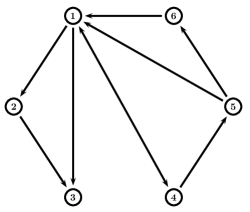
Figure 1: The communication topology.

Consider a group of six spacecraft, whose inertia matrices are shown in Table 1 [15]. The initial attitude states $\sigma_{i}(0)$, $\omega_{i}(0)$, $i=1,2,\cdots,6$, are chosen randomly. The communication topology is given by Fig. 1, so the corresponding adjacency matrix is

$$A=\begin{bmatrix}0&0&0&1&1&1\\ 1&0&0&0&0&0\\ 1&1&0&0&0&0\\ 1&0&0&0&0&0\\ 0&0&0&1&0&0\\ 0&0&0&0&1&0\end{bmatrix}.$$

For (10) and (20), take matrices $\Lambda_{i}=\widehat{\Lambda}_{i}=I_{3}$, $K_{i}=\widehat{K}_{i}=3I_{3}$, $\Gamma_{i}=\widehat{\Gamma}_{i}=3I_{6}$, $i=1,2,\cdots,6$. The parameter estimates $\hat{\theta}_{i}$ and $\hat{\theta}_{fi}$ are initialized to be zero, i.e., $\hat{\theta}_{i}(0)=0$, $\hat{\theta}_{fi}(0)=0$, $i=1,2,\cdots,6$, in (11), (21). For simplicity, let the reference attitude $\sigma^{r}=[0.1,0.3,0.5]^{T}$. Suppose that $\sigma^{r}$ is available only to spacecraft 1. In this case, $a_{17}=1$, $a_{i7}=0$, $i=2,\cdots,6$.

$J_{1}\qquad$	$[1,0.1,0.1;0.1,0.1,0.1;0.1,0.1,0.9]$ kgm2
$J_{2}\qquad$	$[1.5,0.2,0.3;0.2,0.9,0.4;0.3,0.4,2.0]$ kgm2
$J_{3}\qquad$	$[0.8,0.1,0.2;0.1,0.7,0.3;0.2,0.3,1.1]$ kgm2
$J_{4}\qquad$	$[1.2,0.3,0.7;0.3,0.9,0.2;0.7,0.2,1.4]$ kgm2
$J_{5}\qquad$	$[0.9,0.15,0.3;0.15,1.2,0.4;0.3,0.4,1.2]$ kgm2
$J_{6}\qquad$	$[1.1,0.35,0.45;0.35,1.0,0.5;0.45,0.5,1.3]$ kgm2

Table 1: Spacecraft specifications.

Figs. 2(a), 2(b), and 2(c) depict, respectively, the attitudes, angular velocities, and control torques of the six spacecraft with (10) and (11), from which it can be observed that attitude synchronization is indeed achieved. The parameter estimates $\hat{\theta}_{i}$, $i=1,2,\cdots,6$, are shown in Fig. 3. Figs. 4(a), 4(b), 4(c), and 5 depict, respectively, the attitudes, angular velocities, control torques, and the parameter estimates $\hat{\theta}_{fi}$, $i=1,2,\cdots,6$, of the six spacecraft with (20) and (21).

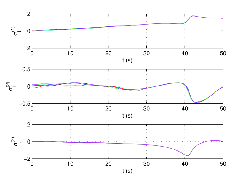
(a) Attitudes

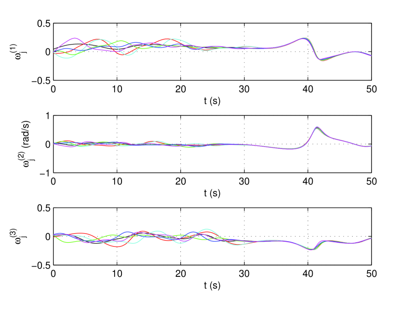
(b) Angular velocities

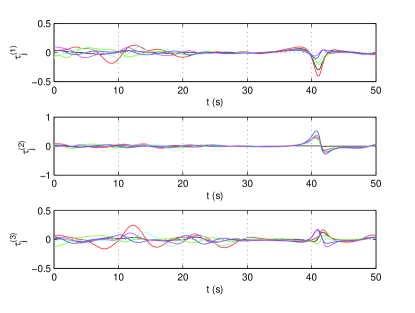
(c) Control torques

Figure 2: Attitudes, angular velocities, and control torques of (1) with controller (10) and adaptive law (11).

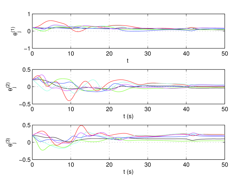
(a) $\hat{\theta}_{i}$, $i=1,2,3$

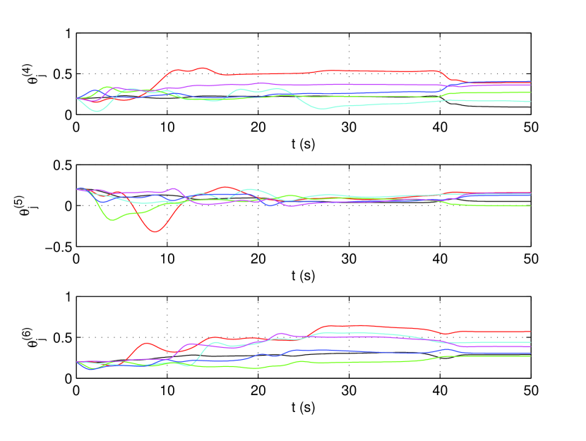
(b) $\hat{\theta}_{i}$, $i=4,5,6$

Figure 3: Parameter estimates of (11).

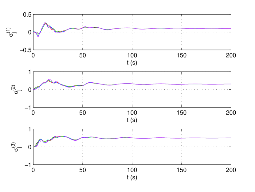
(a) Attitudes

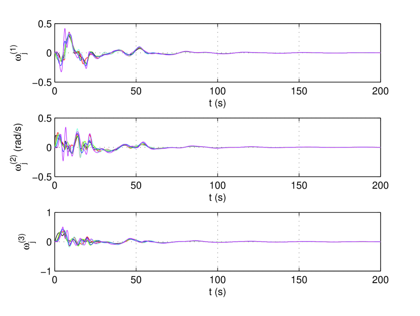
(b) Angular velocities

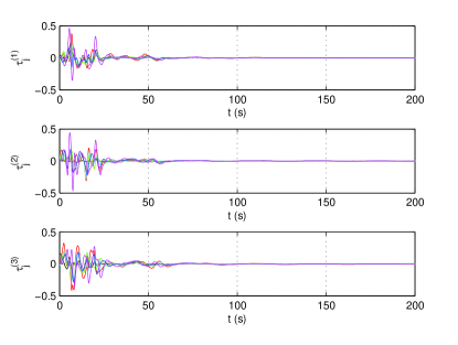
(c) Control torques

Figure 4: Attitudes, angular velocity, and control torques of (1) with controller (20) and adaptive law (21).

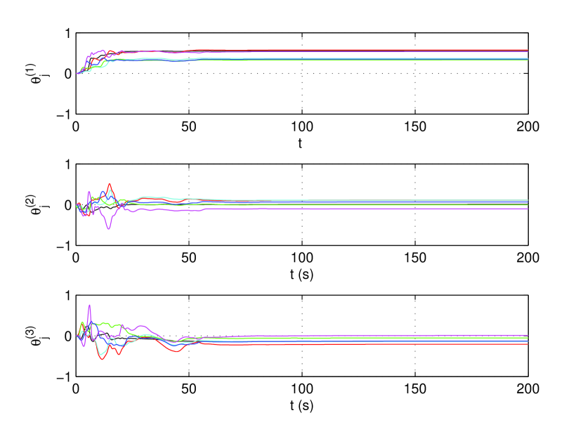
(a) $\hat{\theta}_{fi}$, $i=1,2,3$

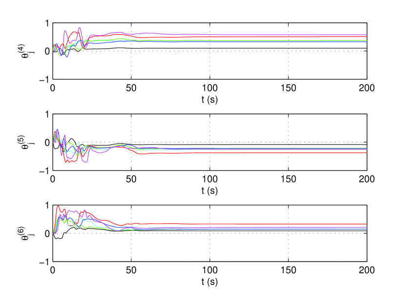
(b) $\hat{\theta}_{fi}$, $i=4,5,6$

Figure 5: Parameter estimates of (21).

6 Conclusions

This paper has addressed the distributed adaptive attitude synchronization problem of a group of spacecraft with unknown inertia matrices. Two distributed adaptive controllers have been proposed for the cases with and without a virtual leader to which a time-varying reference attitude is assigned. The first controller achieves attitude synchronization for a group of spacecraft with a leaderless communication topology having a directed spanning tree. The second controller guarantees that all spacecraft track the reference attitude if the virtual leader has a directed path to all other spacecraft. This paper has extended some existing results in the literature. An interesting topic for future research is the distributed adaptive attitude synchronization of multiple spacecraft without velocity measurements.

References

• [1] A. Abdessameud and A. Tayebi, β€œAttitude synchronization of a group of spacecraft without velocity measurements,” IEEE Transactions on Automatic Control, vol. 54, no. 11, pp. 2642-2648, 2009.
• [2] M. R. Akella, β€œRigid body attitude tracking without angular velocity feedback,” Systems and Control Letters, vol. 42, no. 4, pp. 321-326, 2001.
• [3] L. Cheng, Z. G. Hou, and M. Tan, β€œDecentralized adaptive consensus control for multi-manipulator system with uncertain dynamics,” in Proceedings of IEEE International Conference on Systems, Man, and Cybernetics 2008, pp. 2712-2717.
• [4] S. J. Chung, U. Ahsun, and J.-J. E. Slotine, β€œApplication of synchronization to formation flying spacecraft: Lagrangian approach,” Journal of Guidance, Control, and Dynamics, vol. 32, no. 2, pp. 512-526, 2009.
• [5] D. V. Dimarogonas, P. Tsiotras, and K. J. Kyriakopoulos, β€œLeader-follower cooperative attitude control of multiple rigid bodies,” Systems and Control Letters, vol. 58, no. 6, pp. 429-435, 2009.
• [6] R. A. Horn and C. R. Johnson, Matrix Analysis. Cambridge, UK: Cambridge University Press, 1985.
• [7] J. R. Lawton and R. W. Beard, β€œSynchronize multiple spacecraft rotations,” Automatica, vol. 38, no. 8, pp. 1359-1364, 2002.
• [8] Z. K. Li, Z. S.Β Duan, and L.Β Huang, β€œH∞subscript𝐻H_{\infty} control of networked multi-agent systems,” Journal of Systems Science and Complexity, vol.Β 22, no.Β 1, pp.Β 35-48, 2009.
• [9] Z. K. Li, Z. S. Duan, G. R. Chen, and L. Huang, β€œConsensus of multiagent systems and synchronization of complex networks: A unified viewpoint,” IEEE Transactions on Circuits and Systems I: Regular Papers, vol. 57, no. 1, pp. 213-224, 2010.
• [10] P.Β Lin and Y.Β Jia, β€œDistributed robust $H_{\infty}$ consensus control in directed networks of agents with time-delay,” Systems and Control Letters, vol.Β 57, no.Β 8, pp.Β 643–653, 2008.
• [11] R.Β Olfati-Saber and R. M.Β Murray, β€œConsensus problems in networks of agents with switching topology and time-delays,” IEEE Transactions on Automatic Control, vol.Β 49, no.Β 9, pp.Β 1520–1533, 2004.
• [12] W. Ren and R. W. Beard, β€œDecentralized scheme for spacecraft formation flying via the virtual structure approach,” Journal of Guidance, Control, and Dynamics, vol. 27, no. 1, pp. 73-82, 2004.
• [13] W. Ren and R. W. Beard, β€œConsensus seeking in multiagent systems under dynamically changing interaction topologies,” IEEE Transactions on Automatic Control, vol. 50, no. 5, pp. 655-661, 2005.
• [14] W. Ren, R. W. Beard, and E. M. Atkins. β€œInformation consensus in multivehicle cooperative control,” IEEE Control Systems Magazine, vol. 27, no. 2, pp. 71-82, 2007.
• [15] W. Ren, β€œDistributed attitude alignment in spacecraft formation flying,” International Journal of Adaptive Control and Signal Processing, vol. 21, no. 2-3, pp. 95-113, 2007.
• [16] W. Ren, β€œFormation keeping and attitude alignment for multiple spacecraft through local interactions, Journal of Guidance, Control, and Dynamics, vol. 30, no. 2, pp. 633-638, 2007.
• [17] W. Ren, β€œDistributed cooperative attitude synchronization and tracking for multiple rigid bodies,” IEEE Transactions on Control Systems Technology, vol. 18, no. 2, pp. 383-392, 2010.
• [18] M. D. Shuster, β€œA survey of attitude representation,” Journal of Astronautical Sciences, vol. 41, no. 4, pp. 439-517, 1993.
• [19] J.-J. E. Slotine and W. Li, Applied Nonlinear Control. Englewood Cliffs, New Jersey: Prentice Hall, 1991.
• [20] P. Tsiotras, β€œFurther passivity results for the attitude control problem,” IEEE Transactions on Automatic Control, vol. 43, no. 11, pp. 1597-1600, 1998.
• [21] P. Wang, F. Y. Hadaegh, and K. Lau, β€œSynchronized formation rotation and attitude control of multiple free-flying spacecraft,” Journal of Guidance, Control, and Dynamics, vol. 22, no. 1, pp. 1582-1589, 1999.
• [22] J. T.-Y. Wen and K. Kreutz-Delgado, β€œThe attitude control problem,” IEEE Transactions on Automatic Control, vol. 36, no. 10, pp. 1148-1162, 1991.
• [23] H. Wong, M. S. de Queiroz, and V. Kapila, β€œAdaptive tracking control using synthesized velocity from attitude measurements,” Automatica, vol. 37, no. 6, pp. 947-953, 2001.