Consensus of Discrete-Time Linear Multi-Agent Systems with Observer-Type Protocols

Abstract.

This paper concerns the consensus of discrete-time multi-agent systems with linear or linearized dynamics. An observer-type protocol based on the relative outputs of neighboring agents is proposed. The consensus of such a multi-agent system with a directed communication topology can be cast into the stability of a set of matrices with the same low dimension as that of a single agent. The notion of discrete-time consensus region is then introduced and analyzed. For neurally stable agents, it is shown that there exists an observer-type protocol having a bounded consensus region in the form of an open unit disk, provided that each agent is stabilizable and detectable. An algorithm is further presented to construct a protocol to achieve consensus with respect to all the communication topologies containing a spanning tree. Moreover, for unstable agents, an algorithm is proposed to construct a protocol having an origin-centered disk of radius $\delta$ ($0<\delta<1$) as its consensus region, where $\delta$ has to further satisfy a constraint related to the unstable eigenvalues of a single agent for the case where each agent has a least one eigenvalue outside the unit circle. Finally, the consensus algorithms are applied to solve formation control problems of multi-agent systems.

Zhongkui Li

School of Automation, Beijing Institute of Technology

Beijing 100081, P. R. China

Zhisheng Duan

State Key Lab for Turbulence and Complex Systems

Department of Mechanics and Aerospace Engineering, College of Engineering

Peking University,  Beijing 100871, P. R. China

Guanrong Chen

Department of Electronic Engineering

City University of Hong Kong, Hong Kong, P. R. China

(Dedicated to Professor Qishao Lu with respect and admiration)

1. Introduction

In recent years, the consensus issue of multi-agent systems has received compelling attention from various scientific communities, for its broad applications in such broad areas as satellite formation flying, cooperative unmanned air vehicles, and air traffic control, to name just a few. In [43], a simple model is proposed for phase transition of a group of self-driven particles with numerical demonstration of the complexity of the model. In [11], it provides a theoretical explanation for the behavior observed in [43] by using graph theory. In [22], a general framework of the consensus problem for networks of dynamic agents with fixed or switching topologies is addressed. The conditions given by [22] are further relaxed in [26]. In [8] and [9], tracking control for multi-agent consensus with an active leader is considered, where a local controller is designed together with a neighbor-based state-estimation rule. Some predictive mechanisms are introduced in [47] to achieve ultrafast consensus. In [14, 17], the $H_{\infty}$ consensus and control problems for networks of agents with external disturbances and model uncertainties are investigated. The consensus problems of networks of double-integrator or high-order integrator agents are studied in [18, 28, 29, 36, 40, 45]. A distributed algorithm is proposed in [3] to asymptotically achieve consensus in finite time. The so-called $\epsilon$-consensus problem is considered in [1] for networks of dynamic agents with unknown but bounded disturbances. The average agreement problem is examined in [7] for a network of integrators with quantized links. The controlled agreement problem of multi-agent networks is investigated from a graph-theoretic perspective in [31]. Flocking algorithms are investigated in [23, 38, 39] for a group of autonomous agents. Another topic that is closely related to the consensus of multi-agent systems is the synchronization of coupled nonlinear oscillators, which has been extensively studied, e.g., in [2, 4, 5, 19, 25, 46]. For a relatively complete coverage of the literatures on consensus, readers are referred to the recent surveys [24, 27]. In most existing studies on consensus, the agent dynamics are restricted to be first-, second-, and sometimes high-order integrators, and the proposed consensus protocols are based on the relative states between neighboring agents.

This paper considers the consensus of discrete-time linear multi-agent systems with directed communication topologies. Previous studies along this line include [15, 16, 20, 32, 34, 41, 42, 44]. In [20, 41, 42, 44], static consensus protocols based on relative states of neighboring agents are used. The discrete-time protocol in [32] requires the absolute output measurement of each agent to be available, which is impractical in many cases, e.g., the deep-space formation flying [37]. Contrary to the protocol in [32], an observer-type consensus protocol is proposed here, based only on relative output measurements of neighboring agents, which contains the static consensus protocol developed in [41] as a special case. The observer-type protocol proposed here can be seen as an extension of the traditional observer-based controller for a single system to one for the multi-agent systems. The Separation Principle of the traditional observer-based controllers still holds in the multi-agent setting presented in this paper.

More precisely, a decomposition approach is utilized here to convert the consensus of a multi-agent system, whose communication topology has a spanning tree, into the stability of a set of matrices with the same dimension as a single agent. The final consensus value reached by the agents is derived. Inspired by the notion of continuous-time consensus region introduced in [15] and the synchronized regions of complex networks studied in [4, 19, 25], the notion of discrete-time consensus region is introduced and analyzed. It is pointed out through numerical examples that the consensus protocol should have a reasonably large bounded consensus region so as to be robust to variations of the communication topology. For the special case where the state matrix is neutrally stable, it is shown that there exists an observer-type protocol with a bounded consensus region in the form of an open unit disk, if each agent is stabilizable and detectable. An algorithm is further presented to construct a protocol to achieve consensus with respect to all the communication topologies containing a spanning tree. The main result in [41] can be thereby easily obtained as a corollary. On the contrary, for the general case where the state matrix is unstable, an algorithm is proposed to construct a protocol with the origin-centered disk of radius $\delta$ ($0<\delta<1$) as its consensus region. It is pointed out that $\delta$ has to further satisfy a constraint relying on the unstable eigenvalues of the state matrix for the case where each agent has a least one eigenvalue outside the unit circle, which shows that the consensus problem of the discrete-time multi-agent systems is generally more difficult to solve, compared to the continuous-time case in [15, 16].

In the final, the consensus algorithms are modified to solve formation control problems of multi-agent systems. Previous related works include [6, 13, 30]. In [6], a Nyquist-type criterion is presented to analyze the formation stability. The agent dynamics in [13, 30] are second-order integrators. In this paper, a sufficient condition is given for the existence of a distributed protocol to achieve a specified formation structure for the multi-agent network, which generalizes the results in [13, 30]. Such a protocol can be constructed via the algorithms proposed as above.

The rest of this paper is organized as follows. Notations and some useful results of the graph theory is reviewed in Section 2. The notion of discrete-time consensus region is introduced and analyzed in Section 3. The special case where the state matrix is neutrally stable is considered in Section 4. The case where the state matrix is unstable is investigated in Section 5. The consensus algorithms are applied to formation control of multi-agent systems in Section 6. Section 7 concludes the paper.

2. Notations and Preliminaries

Let $\mathbf{R}^{n\times n}$ and $\mathbf{C}^{n\times n}$ be the sets of $n\times n$ real matrices and complex matrices, respectively. Matrices, if not explicitly stated, have compatible dimensions in all settings. The superscript $T$ means transpose for real matrices and $H$ means conjugate transpose for complex matrices. $\|\cdot\|$ denotes the induced 2-norm. $I_{N}$ represents the identity matrix of dimension $N$, and $I$ the identity matrix of an appropriate dimension. Let $\mathbf{1}\in\mathbf{R}^{p}$ denote the vector with all entries equal to one. For $\zeta\in\mathbf{C}$, $\mathrm{Re}(\zeta)$ denotes its real part. $A\otimes B$ denotes the Kronecker product of matrices $A$ and $B$. The matrix inequality $A>B$ means that $A$ and $B$ are square Hermitian matrices and $A-B$ is positive definite. A matrix $A\in\mathbf{C}^{n\times n}$ is neutrally stable in the discrete-time sense if it has no eigenvalue with magnitude larger than 1 and the Jordan block corresponding to any eigenvalue with unit magnitude is of size one, while is Schur stable if all of its eigenvalues have magnitude less than 1. A matrix $Q\in\mathbf{R}^{n\times n}$ is orthogonal if $QQ^{T}=Q^{T}Q=I$. Matrix $P\in\mathbf{R}^{n\times n}$ is an orthogonal projection onto the subspace ${\rm{range}}(P)$ if $P^{2}=P$ and $P^{T}=P$. Moreover, ${\rm{range}}(A)$ denotes the column space of matrix $A$, i.e, the span of its column vectors.

A directed graph $\mathcal{G}$ is a pair $(\mathcal{V},\mathcal{E})$, where $\mathcal{V}$ is a nonempty finite set of nodes and $\mathcal{E}\subset\mathcal{V}\times\mathcal{V}$ is a set of edges, in which an edge is represented by an ordered pair of distinct nodes. For an edge $(i,j)$, node $i$ is called the parent node, $j$ the child node, and $j$ is neighboring to $i$. A graph with the property that $(i,j)\in\mathcal{E}$ implies $(j,i)\in\mathcal{E}$ is said to be undirected; otherwise, directed. A path on $\mathcal{G}$ from node $i_{1}$ to node $i_{l}$ is a sequence of ordered edges of the form $(i_{k},i_{k+1})$, $k=1,\cdots,l-1$. A directed graph has or contains a directed spanning tree if there exists a node called root such that there exists a directed path from this node to every other node in the graph.

For a graph $\mathcal{G}$ with $m$ nodes, the row-stochastic matrix $\mathcal{D}\in\mathbf{R}^{m\times m}$ is defined with $d_{ii}>0$, $d_{ij}>0$ if $(j,i)\in\mathcal{E}$ but $0$ otherwise, and $\sum_{j=1}^{m}d_{ij}=1$. According to [26], all of the eigenvalues of $\mathcal{D}$ are either in the open unit disk or equal to $1$, and furthermore, $1$ is a simple eigenvalue of $\mathcal{D}$ if and only if graph $\mathcal{G}$ contains a directed spanning tree. For an undirected graph, $\mathcal{D}$ is symmetric.

Let $\Gamma_{m}$ denote the set of all directed graphs with $m$ nodes such that each graph contains a directed spanning tree, and let $\Gamma_{\leq\delta}$ ($0<\delta<1$) denote the set of all directed graphs containing a directed spanning tree, whose non-one eigenvalues lie in the disk of radius $\delta$ centered at the origin.

2.1. Problem Formulation

Consider a network of $N$ identical agent with linear or linearized dynamics in the discrete-time setting, where the dynamics of the $i$-th agent are described by

$$x_{i}^{+} =Ax_{i}+Bu_{i},$$ (1)

$$y_{i} =Cx_{i},\quad i=1,2,\cdots,N,$$

where $x_{i}=x_{i}(k)=[x_{i,1},\cdots,x_{i,n}]\in\mathbf{R}^{n\times n}$ is the state, $x_{i}^{+}=x_{i}(k+1)$ is the state at the next time instant, $u_{i}\in\mathbf{R}^{p}$ is the control input, $y_{i}\in\mathbf{R}^{q}$ is the measured output, and $A$, $B$, $C$ are constant matrices with compatible dimensions.

The communication topology among agents is represented by a directed graph $\mathcal{G}=(\mathcal{V},\mathcal{E})$, where $\mathcal{V}=\{1,\cdots,N\}$ is the set of nodes (i.e., agents) and $\mathcal{E}\subset\mathcal{V}\times\mathcal{V}$ is the set of edges. An edge $(i,j)$ in graph $\mathcal{G}$ means that agent $j$ can obtain information from agent $i$, but not conversely.

At each time instant, the information available to agent $i$ is the relative measurements of other agents with respect to itself, given by

$$\zeta_{i}=\sum_{j=1}^{N}d_{ij}(y_{i}-y_{j}),$$ (2)

where $\mathcal{D}=(d_{ii})_{N\times N}$ is the row-stochastic matrix associated with graph $\mathcal{G}$. A distributed observer-type consensus protocol is proposed as

$$v_{i}^{+} =(A+BK)v_{i}+L\left(\sum_{j=1}^{N}d_{ij}C(v_{i}-v_{j})-\zeta_{i}\right),$$ (3)

$$u_{i} =Kv_{i},$$

where $v_{i}\in\mathbf{R}^{n}$ is the protocol state, $i=1,\cdots,N$, $L\in\mathbf{R}^{q\times n}$ and $K\in\mathbf{R}^{p\times n}$ are feedback gain matrices to be determined. In (3), the term $\sum_{j=1}^{N}d_{ij}C(v_{i}-v_{j})$ denotes the information exchanges between the protocol of agent $i$ and those of its neighboring agents. It is observed that the protocol (3) maintains the same communication topology as the agents in (1).

Let $z_{i}=[x_{i}^{T},v_{i}^{T}]^{T}$ and $z=[z_{1}^{T},\cdots,z_{N}^{T}]^{T}$. Then, the closed-loop system resulting from (1) and (3) can be written as

$$z^{+}=(I_{N}\otimes\mathcal{A}+(I_{N}-\mathcal{D})\otimes\mathcal{H})z,$$ (4)

where

$$\mathcal{A}=\begin{bmatrix}A&BK\\ 0&A+BK\end{bmatrix},\quad\mathcal{H}=\begin{bmatrix}0&0\\ -LC&LC\end{bmatrix}.$$

Definition 2.1.

Given agents (1), the protocol (3) is said to solve the consensus problem if

$$\|x_{i}(k)-x_{j}(k)\|\rightarrow 0,~{}\text{as}~{}k\rightarrow\infty,~{}\forall~{}i,j=1,2,\cdots,N.$$ (5)

The following presents a decomposition approach to the consensus problem of network (4).

Theorem 2.2.

For any $\mathcal{G}\in\Gamma_{N}$, the agents in (1) reach consensus under protocol (3) if all the matrices $A+BK$, $A+(1-\lambda_{i})LC$, $i=2,\cdots,N$, are Schur stable, where $\lambda_{i}$, $i=2,\cdots,N$, denote the eigenvalues of $\mathcal{D}$ located in the open unit disk.

Proof.

For any $\mathcal{G}\in\Gamma_{N}$, it is known that $0$ is a simple eigenvalue of $I_{N}-\mathcal{D}$ and the other eigenvalues lie in the open unit disk centered at $1+{\rm i}0$ in the complex plane, where ${\rm i}=\sqrt{-1}$. Let $r^{T}\in\mathbf{R}^{1\times N}$ be the left eigenvector of $I_{N}-\mathcal{D}$ associated with the eigenvalue $0$, satisfying $r^{T}{\bf 1}=1$. Introduce $\xi\in\mathbf{R}^{2Nn\times 2Nn}$ by

$$\xi(t) =z(t)-\left(({\bf 1}r^{T})\otimes I_{2n}\right)z(t)$$ (6)

$$=\left((I_{N}-{\bf 1}r^{T})\otimes I_{2n}\right)z(t),$$

which satisfies $(r^{T}\otimes I_{2n})\xi=0$. It is easy to see that $0$ is a simple eigenvalue of $I_{N}-{\bf 1}r^{T}$ with $\mathbf{1}$ as its right eigenvector, and 1 is another eigenvalue with multiplicity $N-1$. Thus, it follows from (6) that $\xi=0$ if and only if $z_{1}=z_{2}=\cdots=z_{N}$, i.e., the consensus problem can be cast into the Schur stability of vector $\xi$, which evolves according to the following dynamics:

$$\xi^{+}=(I_{N}\otimes\mathcal{A}+(I-\mathcal{D})\otimes\mathcal{H})\xi.$$ (7)

Next, let $Y\in\mathbf{R}^{N\times(N-1)}$, $W\in\mathbf{R}^{(N-1)\times N}$, $T\in\mathbf{R}^{N\times N}$, and upper-triangular $\Delta\in\mathbf{R}^{(N-1)\times(N-1)}$ be such that

$$T=\begin{bmatrix}\mathbf{1}&Y\end{bmatrix},\quad T^{-1}=\begin{bmatrix}r^{T}\\ W\end{bmatrix},\quad T^{-1}(I_{N}-\mathcal{D})T=J=\begin{bmatrix}0&0\\ 0&\Delta\end{bmatrix},$$ (8)

where the diagonal entries of $\Delta$ are the nonzero eigenvalues of $I_{N}-\mathcal{D}$. Introduce the state transformation $\zeta=(T^{-1}\otimes I_{2n})\xi$ with $\zeta=[\zeta_{1}^{T},\cdots,\zeta_{N}^{T}]^{T}$. Then, (7) can be represented in terms of $\zeta$ as follows:

$$\zeta^{+}=(I_{N}\otimes\mathcal{A}+J\otimes\mathcal{H})\zeta.$$ (9)

As to $\zeta_{1}$, it can be seen from (6) that

$$\zeta_{1}=(r^{T}\otimes I_{2n})\xi\equiv 0.$$ (10)

Note that the elements of the state matrix of (9) are either block diagonal or block upper-triangular. Hence, $\zeta_{i},$ $i=2,\cdots,N$, converge asymptotically to zero if and only if the $N-1$ subsystems along the diagonal, i.e.,

$$\zeta^{+}_{i}=(\mathcal{A}+(1-\lambda_{i})\mathcal{H})\zeta_{i},\quad i=2,\cdots,N,$$ (11)

are Schur stable. It is easy to verify that matrices $\mathcal{A}+\lambda_{i}\mathcal{H}$ are similar to

$$\begin{bmatrix}A+(1-\lambda_{i})LC&0\\ -(1-\lambda_{i})LC&A+BK\end{bmatrix},\quad i=2,\cdots,N.$$

Therefore, the Schur stability of the matrices $A+BK$, $A+(1-\lambda_{i})LC$, $i=2,\cdots,N$, is equivalent to that the state $\zeta$ of (7) converges asymptotically to zero, implying that consensus is achieved. ∎

Remark 1.

The importance of this theorem lies in that it converts the consensus problem of a large-scale therefore very high-dimensional multi-agent network under the observer-type protocol (3) to the stability of a set of matrices with the same dimension as a single agent, thereby significantly reducing the computational complexity. The directed communication topology $\mathcal{G}$ is only assumed to have a directed spanning tree. The effects of the communication topology on the consensus problem are characterized by the eigenvalues of the corresponding row-stochastic matrix $\mathcal{D}$, which may be complex, rendering the matrices be complex-valued in Theorem 2.2.

Remark 2.

The observer-type consensus protocol (3) can be seen as an extension of the traditional observer-based controller for a single system to one for multi-agent systems. The Separation Principle of the traditional observer-based controllers still holds in this multi-agent setting. Moreover, the protocol (3) is based only on relative output measurements between neighboring agents, which can be regarded as the discrete-time counterpart of the protocol proposed in [15, 16], including the static protocol used in [41] as a special case.

Theorem 2.3.

Consider the multi-agent network (4) with a communication topology $\mathcal{G}\in\Gamma_{N}$. If protocol (3) satisfies Theorem 2.2, then

$$x_{i}(k) \rightarrow\varpi(k)\triangleq(r^{T}\otimes A^{k})\begin{bmatrix}x_{1}(0)\\ \vdots\\ x_{N}(0)\end{bmatrix},$$ (12)

$$v_{i}(k) \rightarrow 0,~{}i=1,2,\cdots,N,~{}\text{ as}~{}k\rightarrow\infty,$$

where $r\in\mathbf{R}^{N}$ satisfies $r^{T}(I_{N}-\mathcal{D})=0$ and $r^{T}{\bf 1}=1$.

Proof.

The solution of (4) can be obtained as

$$z(k+1) =\left(I_{N}\otimes\mathcal{A}+(I_{N}-\mathcal{D})\otimes\mathcal{H}\right)^{k}z(0)$$

$$=(T\otimes I)(I_{N}\otimes\mathcal{A}+J\otimes\mathcal{H})^{k}(T^{-1}\otimes I)z(0)$$

$$=(T\otimes I)\begin{bmatrix}\mathcal{A}^{k}&0\\ 0&(I_{N-1}\otimes\mathcal{A}+\Delta\otimes\mathcal{H})^{k}\end{bmatrix}(T^{-1}\otimes I)z(0),$$

where matrices $T$, $J$ and $\Delta$ are defined in (8). By Theorem 2.2, $I_{N-1}\otimes\mathcal{A}+\Delta\otimes\mathcal{H}$ is Schur stable. Thus,

$$z(k+1) \rightarrow(\mathbf{1}\otimes I)\mathcal{A}^{k}(r^{T}\otimes I)z(0)$$

$$=(\mathbf{1}r^{T})\otimes\mathcal{A}^{k}z(0),~{}\text{ as}~{}k\rightarrow\infty,$$

implying that

$$z_{i}(k)\rightarrow(r^{T}\otimes\mathcal{A}^{k})z(0),~{}\text{ as}~{}k\rightarrow\infty,~{}i=1,\cdots,N.$$ (13)

Since $A+BK$ is Schur stable, (13) directly leads to the assertion. ∎

Remark 3.

Some observations on the final consensus value in (12) can be concluded as follows: If $A$ is Schur stable, then $\varpi(k)\rightarrow 0$, as $k\rightarrow\infty$. If $A$ in (1) has eigenvalues located outside the open unit circle, then the consensus value $\varpi(k)$ reached by the agents will tend to infinity exponentially. On the other hand, if $A$ has eigenvalues in the closed unit circle, then the agents in (1) may reach consensus nontrivially. That is, some states of each agent might approach a common nonzero value. Typical examples belonging to the last case include the commonly-studied first-, second-, and high-order integrators.

3. Discrete-Time Consensus Regions

From Theorem (2.2), it can be noticed that the consensus of the given agents (1) under protocol (3) depends on the feedback gain matrices $K$, $L$, and the eigenvalues $\lambda_{i}$ of matrix $\mathcal{D}$ associated with the communication graph $\mathcal{G}$, where matrix $L$ is coupled with $\lambda_{i}$, $i=2,\cdots,N$. Hence, it is useful to analyze the correlated effects of matrix $L$ and graph $\mathcal{G}$ on consensus. To this end, the notion of consensus region is introduced.

Definition 2. Assume that matrix $K$ has been designed such that $A+BK$ is Schur stable. The region $\mathcal{S}$ of the parameter $\sigma\subset\mathbf{C}$, such that matrix $A+(1-\sigma)LC$ is Schur stable, is called the (discrete-time) consensus region of network (4).

The notion of discrete-time consensus region is inspired by the continuous-time consensus region introduced in [15] and the synchronized regions of complex networks studied in [4, 19, 25]. The following result is a direct consequence of Theorem 2.2.

Corollary 1.

The agents in (1) reach consensus under protocol (3) if $\lambda_{i}\in\mathcal{S}$, $i=2,\cdots,N$, where $\lambda_{i}$, $i=2,\cdots,N$, are the eigenvalues of $\mathcal{D}$ located in the open unit disk.

For an undirected communication graph, the consensus region of network (4) is a bounded interval or a union of several intervals on the real axis. However, for a directed graph where the eigenvalues of $\mathcal{D}$ are generally complex numbers, the consensus region $\mathcal{S}$ is either a bounded region or a set of several disconnected regions in the complex plane. Due to the fact that the eigenvalues of the row-stochastic matrix $\mathcal{D}$ lie in the unit disk, unbounded consensus regions, desirable for consensus in the continuous-time setting [15, 16], generally do not exist for the discrete-time consensus considered here.

The following example has a disconnected consensus region.

Example 1. The agent dynamics and the consensus protocol are given by (1) and (3), respectively, with

$$A =\begin{bmatrix}0&1\\ -1&1.02\end{bmatrix},\quad B=\begin{bmatrix}1\\ 0\end{bmatrix},\quad C=\begin{bmatrix}1&0\\ 0&1\end{bmatrix},$$

$$L =\begin{bmatrix}0&-1\\ 1&0\end{bmatrix},\quad K=\begin{bmatrix}-0.5&-0.5\end{bmatrix}.$$

Clearly, matrix $A+BK$ with $K$ given as above is Schur stable. For simplicity in illustration, assume that the communication graph $\mathcal{G}$ is undirected here. Then, the consensus region is a set of intervals on the real axis. The characteristic equation of $A+(1-\sigma)LC$ is

$${\rm{det}}(zI-A-\sigma LC)=z^{2}-1.02z+\sigma^{2}=0.$$ (14)

Applying bilinear transformation $z=\frac{s+1}{s-1}$ to (14) gives

$$(\sigma^{2}-0.02)s^{2}+(1-\sigma^{2})s+2.02+\sigma^{2}=0.$$ (15)

It is well known that, under the bilinear transformation, (14) has all roots within the unit disk if and only if the roots of (15) lie in the open left-half plane (LHP). According to the Hurwitz criterion [21], (15) has all roots in the open LHP if and only if $0.02<\sigma^{2}<1$. Therefore, the consensus region in this case is $\mathcal{S}=(-1,-0.1414)\cup(0.1414,1)$, a union of two disconnected intervals. For the communication graph shown in Figure 1, the corresponding row-stochastic matrix is

$$\mathcal{D}=\begin{bmatrix}0.3&0.2&0.2&0.2&0&0.1\\ 0.2&0.6&0.2&0&0&0\\ 0.2&0.2&0.6&0&0&0\\ 0.2&0&0&0.4&0.4&0\\ 0&0&0&0.4&0.2&0.4\\ 0.1&0&0&0&0.4&0.5\end{bmatrix},$$

whose eigenvalues, other than 1, are $-0.2935,0.164,0.4,0.4624,0.868$, which all belong to $\mathcal{S}$. Thus, it follows from Corollary 1 that network (4) with graph given in Figure 1 can achieve consensus.

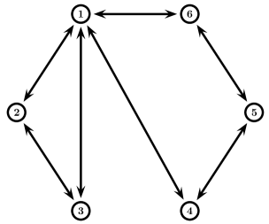
Figure 1. The communication topology.

Let’s see how modifications of the communication topology affect the consensus. Consider the following two simple cases:

1) An edge is added between nodes 1 and 5, thus more information exchange will exist inside the network. Then, the row-stochastic matrix $\mathcal{D}$ becomes

$$\begin{bmatrix}0.2&0.2&0.2&0.2&0.1&0.1\\ 0.2&0.6&0.2&0&0&0\\ 0.2&0.2&0.6&0&0&0\\ 0.2&0&0&0.4&0.4&0\\ 0.1&0&0&0.4&0.2&0.3\\ 0.1&0&0&0&0.4&0.5\end{bmatrix},$$

whose eigenvalues, in addition to 1, are $-0.2346,0.0352,0.4,0.4634,0.836$. Clearly, the eigenvalue $0.0352$ does not belong to $\mathcal{S}$, i.e., consensus can not be achieved in this case.

2) The edge between nodes 5 and 6 is removed. The row-stochastic matrix $\mathcal{D}$ becomes

$$\begin{bmatrix}0.3&0.2&0.2&0.2&0&0.1\\ 0.2&0.6&0.2&0&0&0\\ 0.2&0.2&0.6&0&0&0\\ 0.2&0&0&0.4&0.4&0\\ 0.1&0&0&0.4&0.6&0\\ 0.1&0&0&0&0&0.9\end{bmatrix},$$

whose eigenvalues, other than 1, are $-0.0315,0.2587,0.4,0.8676,0.9052$. In this case, the eigenvalue $-0.0315$ does not belong to $\mathcal{S}$, i.e., consensus can not be achieved either.

These sample cases imply that, for disconnected consensus regions, consensus can be quite fragile to the variations of the network’s communication topology. Hence, the consensus protocol should be designed to have a sufficiently large bounded consensus region in order to be robust with respect to the communication topology. This is the topic of the following sections.

4. Networks with Neurally Stable Agents

In this section, a special case where matrix $A$ is neutrally stable is considered. First, the following lemma is needed.

Lemma 4.1 ([48]).

For matrix $Q=Q^{H}\in\mathbf{C}^{n\times n}$, consider the following Lyapunov equation:

$$A^{H}XA-X+Q=0.$$

If $X>0$, $Q\geq 0$, and $(Q,V)$ is observable, then matrix $A$ is Schur stable .

Proposition 1.

For matrices $Q\in\mathbf{R}^{n\times n}$, $V\in\mathbf{R}^{m\times n}$, $\sigma\in\mathbf{C}$, where $Q$ is orthogonal, $VV^{T}=I$, and $(Q,V)$ is observable, if $|\sigma|<1$, then the matrix $Q-(1-\sigma)QV^{T}V$ is Schur stable.

Proof.

Observe that

$$(Q-(1-\sigma)QV^{T}V)^{H}(Q-(1-\sigma)QV^{T}V)-I$$ (16)

$$\qquad=Q^{T}Q-(1-\sigma)Q^{T}QV^{T}V-(1-\bar{\sigma})V^{T}VQ^{T}Q$$

$$\qquad\quad+|1-\sigma|^{2}V^{T}VQ^{T}QV^{T}V-I$$

$$\qquad=(-2\mathbf{Re}(1-\sigma)+|1-\sigma|^{2})V^{T}V$$

$$\qquad=(|\sigma|^{2}-1)V^{T}V.$$

Since $(Q,V)$ is observable, it is easy to verify that $(Q-(1-\sigma)QV^{T}V,V^{T}V)$ is also observable. Then, by Lemma 4.1, (16) implies that $Q-(1-\sigma)QV^{T}V$ is Schur stable for any $|\sigma|<1$. ∎

Next, an algorithm for protocol (3) is presented, which will be used later.

Algorithm 1. Given that $A$ is neutrally stable and that $(A,B,C)$ is stabilizable and detectable, the protocol (3) can be constructed as follows:

• Select $K$ be such that $A+BK$ is Schur stable.

• Choose $U\in\mathbf{R}^{n\times n_{1}}$ and $W\in\mathbf{R}^{n\times(n-n_{1})}$, satisfying

  $$\begin{bmatrix}U&W\end{bmatrix}^{-1}A\begin{bmatrix}U&W\end{bmatrix}=\begin{bmatrix}M&0\\ 0&X\end{bmatrix},$$ (17)

  where $M\in\mathbf{R}^{n_{1}\times n_{1}}$ is orthogonal and $X\in\mathbf{R}^{(n-n_{1})\times(n-n_{1})}$ is Schur stable.

• Choose $V\in\mathbf{R}^{m\times n_{1}}$ such that $VV^{T}=I_{m}$ and $\mathrm{range}(V^{T})=\mathrm{range}(U^{T}C^{T})$.

• Define $L=-UMV^{T}(CUV^{T})^{-1}$.

Theorem 4.2.

Suppose that matrix $A$ is neutrally stable and that $(A,B,C)$ is stabilizable and detectable. The protocol (3) constructed via Algorithm 1 has the open unit disk as its bounded consensus region. Thus, such a protocol solves the consensus problem for (1) with respect to $\Gamma_{N}$, the set of all the communication topologies containing a spanning tree.

Proof.

Let the related variables be defined as in Algorithm 1. Assume without loss of generality that matrix $CU$ is of full row rank. Since $V^{T}V$ is an orthogonal projection onto $\mathrm{range}(V^{T})=\mathrm{range}(U^{T}C^{T})$, matrix $CUV^{T}$ is invertible and $V^{T}VU^{T}C^{T}=U^{T}C^{T}$, so that $V=(CUV^{T})^{-1}CU$, and hence $LCU=-UMV^{T}V$. Also, the detectability of $(A,C)$ implies that $(M,V)$ is observable. Let $U^{{\dagger}}\in\mathbf{R}^{n_{1}\times n}$ and $W^{{\dagger}}\in\mathbf{R}^{(n-n_{1})\times n}$ be such that $\begin{bmatrix}U^{{\dagger}}\\ W^{{\dagger}}\end{bmatrix}=\begin{bmatrix}U&W\end{bmatrix}^{-1},$ where $U^{{\dagger}}U=I$, $W^{{\dagger}}W=I$, $U^{{\dagger}}W=0$, and $W^{{\dagger}}U=0$. Then,

$$\begin{bmatrix}U&U\end{bmatrix}^{-1}(A+(1-\sigma)LC)\begin{bmatrix}U&W\end{bmatrix}$$ (18)

$$=\begin{bmatrix}M+(1-\sigma)U^{{\dagger}}LCU&(1-\sigma)U^{{\dagger}}LCW\\ (1-\sigma)W^{{\dagger}}LCU&X+(1-\sigma)W^{{\dagger}}LCW\end{bmatrix}$$

$$=\begin{bmatrix}M-(1-\sigma)MV^{T}V&-(1-\sigma)U^{{\dagger}}LCW\\ 0&X\end{bmatrix}.$$

By Lemma 4.1, matrix $M-(1-\sigma)MV^{T}V$ is Schur stable for any $|\sigma|<1$. Hence, (18) implies that matrix $A+(1-\sigma)LC$ with $L$ given by Algorithm 1 is Schur stable for any $|\sigma|<1$, i.e., the protocol (3) constructed via Algorithm 1 has a bounded consensus region in the form of the open unit disk. Since the eigenvalues of any communication topology containing a spanning tree lie in the open unit disk, except eigenvalue 1, it follows from Corollary 1 that this protocol solves the consensus problem with respect to $\Gamma_{N}$. ∎

In [41], the consensus of the following coupled network is considered:

$$x_{i}^{+}=Ax_{i}+LC\sum_{j=1}^{N}d_{ij}(x_{i}-x_{j}),\quad i=1,2\cdots,N,$$ (19)

where $(d_{ij})_{N\times N}$ is defined as in (2) and matrix $L$ is to be designed.

The main result of [41] can be easily obtained as a corollary here.

Corollary 2.

There exists a matrix $L$ such that network (19) has the open unit disk as its consensus region, i.e., the network can reach consensus with respect to $\Gamma_{N}$, if and only if the pair $(A,C)$ is detectable. Such a matrix $L$ can be constructed via Algorithm 1.

Proof.

For any communication topology $\mathcal{G}\in\Gamma_{N}$, it follows from Theorem 2.2 that there exists a matrix $L$ such that network (19) achieves consensus if and only if matrices $A+(1-\lambda_{i})LC$, $i=2,\cdots,N$, are Schur stable. The necessity is obvious and the sufficiency follows readily from Theorem 4.2. ∎

Remark 4.

Compared to Theorem 6 in [41], the above corollary presents a necessary and sufficient condition for the existence of a matrix $L$ that ensures the network to reach consensus. Moreover, the method leading to this corollary is quite different from and comparatively much simpler than that used in [41]. Of course, it should be admitted that the proof of Theorem 4.2 above is partly inspired by [41].

Example 2. Consider a network of agents described by (1), with

$$A=\begin{bmatrix}0.2&0.6&0\\ -1.4&0.8&0\\ 0.7&0.2&-0.5\end{bmatrix},\quad B=\begin{bmatrix}0\\ 1\\ 0\end{bmatrix},\quad C=\begin{bmatrix}1&0&1\end{bmatrix}.$$

The eigenvalues of matrix $A$ are $-0.5$, $0.5\pm{\rm i}0.866$, thus $A$ is neutrally stable. In protocol (3), choose $K=\left[\begin{matrix}1.2&-0.9&-0.2\end{matrix}\right]$ such that $A+BK$ is Schur stable. The matrices

$$U=\begin{bmatrix}0.1709&-0.4935\\ 0.7977&0\\ -0.0570&-0.2961\end{bmatrix},\quad W=\begin{bmatrix}0\\ 0\\ 1\end{bmatrix}$$

satisfy (17) with $M=\left[\begin{smallmatrix}0.5&0.866\\ -0.866&0.5\end{smallmatrix}\right]$ and $X=-0.5$. Thus, $U^{T}C^{T}=\left[\begin{smallmatrix}0.1139&-0.7896\end{smallmatrix}\right]^{T}$. Take $V=\left[\begin{matrix}0.1428&-0.9898\end{matrix}\right]$ such that $VV^{T}=1$ and ${\rm{range}}(V^{T})={\rm{range}}(U^{T}C^{T})$. Then, by Algorithm 1, one obtains $L=\left[\begin{matrix}-0.2143&0.7857&-0.2857\end{matrix}\right]^{T}$. In light of Theorem 4.2, the agents considered in this example will reach consensus under the protocol (3), with $K$ and $L$ given as above, with respect to all the communication topologies containing a spanning tree.

5. Networks with Unstable Agents

This section considers the general case where matrix $A$ is not neutrally stable, i.e., $A$ is allowed to have eigenvalues outside the unit circle or has at least one eigenvalue with unit magnitude whose corresponding Jordan block is of size larger than 1.

Before moving forward, one introduces the following modified algebraic Riccati equation (MARE) [12, 33, 35]:

$$P=APA^{T}-(1-\delta^{2})APC^{T}(CPC^{T}+I)^{-1}CPA^{T}+Q,$$ (20)

where $P\geq 0$, $Q>0$, and $\delta\in\mathbf{R}$. For $\delta=0$, the MARE (20) is reduced to the commonly-used discrete-time Riccati equation discussed in, e.g., [48].

The following lemma concerns the existence of solutions for the MARE.

Lemma 5.1 ([33, 35]).

Let $(A,C)$ be detectable. Then, the following statements hold.

• Suppose that the matrix $A$ has no eigenvalues with magnitude larger than 1, Then, the MARE (20) has a unique positive-definite solution $P$ for any $0<\delta<1$.

• For the case where $A$ has a least one eigenvalue with magnitude larger than 1 and the rank of $B$ is one, the MARE (20) has a unique positive-definite solution $P$, if $0<\delta<\frac{1}{\underset{i}{\Pi}|\lambda_{i}^{u}(A)|}$, where $\lambda_{i}^{u}(A)$ denote the unstable eigenvalues of $A$.

• If the MARE (20) has a unique positive-definite solution $P$, then $P=\lim_{k\rightarrow\infty}P_{k}$ for any initial condition $P_{0}\geq 0$, where $P_{k}$ satisfies

  $$P(k+1)=AP(k)A^{T}-(1-\delta^{2})AP(k)C^{T}(CP(k)C^{T}+I)^{-1}CP(k)A^{T}+Q.$$

Proposition 2.

Suppose that $(A,C)$ be detectable. Then, for the case where $A$ has no eigenvalues with magnitude larger than 1, the matrix $A+(1-\sigma)LC$ with $L=-APC^{T}(CPC^{T}+I)^{-1}$ is Schur stable for any $|\sigma|\leq\delta$, $0<\delta<1$, where $P>0$ is the unique solution to the MARE (20). Moreover, for the case where $A$ has at least eigenvalue with magnitude larger than 1 and $B$ is of rank one, $A+(1-\sigma)LC$ with $L=-APC^{T}(CPC^{T}+I)^{-1}$ is Schur stable for any $|\sigma|\leq\delta$, $0<\delta<\frac{1}{\underset{i}{\Pi}|\lambda_{i}^{u}(A)|}$.

Proof.

Observe that

$$(A+(1-\sigma)LC)P(A+(1-\sigma)LC)^{H}-P$$ (21)

$$=APA^{T}-2\mathbf{Re}(1-\sigma)APC^{T}(CPC^{T}+I)^{-1}CPA^{T}-P$$

$$\quad+|1-\sigma|^{2}APC^{T}(CPC^{T}+I)^{-1}CPC^{T}(CPC^{T}+I)^{-1}CPA^{T}$$

$$=APA^{T}+(-2\mathbf{Re}(1-\sigma)+|1-\sigma|^{2})APC^{T}(CPC^{T}+I)^{-1}CPA^{T}-P$$

$$\quad+|1-\sigma|^{2}APC^{T}(CPC^{T}+I)^{-1}\left(-I+CPC^{T}(CPC^{T}+I)^{-1}\right)CPA^{T}$$

$$=APA^{T}+(|\sigma|^{2}-1)APC^{T}(CPC^{T}+I)^{-1}CPA^{T}-P$$

$$\quad-|1-\sigma|^{2}APC^{T}(CPC^{T}+I)^{-2}CPA^{T}$$

$$\leq APA^{T}-(1-\delta^{2})APC^{T}(CPC^{T}+I)^{-1}CPA^{T}-P$$

$$=-Q<0,$$

where the identity $-I+CPC^{T}(CPC^{T}+I)^{-1}=-(CPC^{T}+I)^{-1}$ has been applied. Then, the assertion follows directly from Lemma 5.1 and the discrete-time Lyapunov inequality. ∎

Algorithm 2. Assuming that $(A,B,C)$ is stabilizable and detectable, the protocol (3) can the constructed as follows:

• Select $K$ such that $A+BK$ is Schur stable.

• Choose $L=-APC^{T}(CPC^{T}+I)^{-1}$, where $P>0$ is the unique solution of (20).

Remark 5.

By Lemma 5.1 and Proposition 2, it follows that a sufficient and necessary condition for the existence of the consensus protocol by using Algorithm 2 is that $(A,B,C)$ is stabilizable and detectable for the case where $A$ has no eigenvalues with magnitude larger than 1. In contrast, $\delta$ has to further satisfy $\delta<\frac{1}{\underset{i}{\Pi}|\lambda_{i}^{u}(A)|}$ for the case where $A$ has at least eigenvalue outside the unit circle and $B$ is of rank one.

The result below follows directly from Theorem 2.3 and Proposition 2.

Theorem 5.2.

Let $(A,B,C)$ be stabilizable and detectable. Then, the protocol given by Algorithm 2 has a bounded consensus region in the form of an origin-centered disk of radius $\delta$, i.e., this protocol solves the consensus problem for networks with agents (1) with respect to $\Gamma_{\leq\delta}$, where $\delta$ satisfies $0<\delta<1$ for the case where $A$ has no eigenvalues with magnitude larger than 1 and satisfies $0<\delta<\frac{1}{\underset{i}{\Pi}|\lambda_{i}^{u}(A)|}$ for the case where $A$ has a least one eigenvalue outside the unit circle and $B$ is of rank one.

Remark 6.

Note that $\Gamma_{\leq\delta}$ was defined in Section 2, which is a subset of $\Gamma_{m}$ in the special case where $A$ is neutrally stable as discussed in the above section. This is consistent with the intuition that unstable behaviors are more difficult to synchronize than the neutrally stable ones.

Example 3. Let the agents in (1) be discrete-time double integrators, with

$$A=\begin{bmatrix}1&1\\ 0&1\end{bmatrix},\quad B=\begin{bmatrix}0\\ 1\end{bmatrix},\quad C=\begin{bmatrix}1&0\end{bmatrix}.$$

Obviously, Assumption 1 holds here. Choose $K=\left[\begin{matrix}-0.5&-1.5\end{matrix}\right]$, so that matrix $A+BK$ is Schur stable. Solving equation (20) with $\delta=0.95$ gives $P=10^{4}\times\begin{bmatrix}1.1780&0.0602\\ 0.0602&0.0062\end{bmatrix}$. By Algorithm 2, one obtains $L=\left[\begin{matrix}-1.051&-0.051\end{matrix}\right]^{T}$. It follows from Theorem 5.2 that the agents (1) reach consensus under protocol (3) with $K$ and $L$ given as above with respect to $\Gamma_{\leq 0.95}$. Assume that the communication topology $\mathcal{G}$ is given as in Figure 2, and the corresponding row-stochastic matrix is

$$\mathcal{D}=\begin{bmatrix}0.4&0&0&0.1&0.3&0.2\\ 0.5&0.5&0&0&0&0\\ 0.3&0.2&0.5&0&0&0\\ 0.5&0&0&0.5&0&0\\ 0&0&0&0.4&0.4&0.2\\ 0&0&0&0&0.3&0.7\end{bmatrix},$$

whose eigenvalues, other than 1, are $\lambda_{i}=0.5,0.5565,0.2217\pm{\rm i}0.2531$. Clearly, $|\lambda_{i}|<0.95$, for $i=2,\cdots,6$. Figure 3 depicts the state trajectories of network (4) for this example, which shows that consensus is actually achieved.

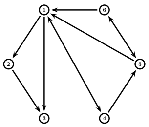
Figure 2. The communication topology.

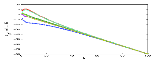
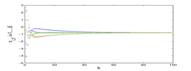
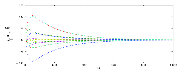
Figure 3. The state trajectories of a double-integrator network.

6. Application to Formation Control

In this section, the consensus algorithms are modified to solve formation control problems of multi-agent systems.

Let $\widetilde{H}=(h_{1},h_{2},\cdots,h_{N})\in\mathbf{R}^{n\times N}$ describe a constant formation structure of the agent network in a reference coordinate frame, where $h_{i}\in\mathbf{R}^{n}$, is the formation variable corresponding to agent $i$. For example, $h_{1}=\left[\begin{matrix}0&0\end{matrix}\right]^{T}$, $h_{2}=\left[\begin{matrix}0&1\end{matrix}\right]^{T}$, $h_{3}=\left[\begin{matrix}1&0\end{matrix}\right]^{T}$, and $h_{4}=\left[\begin{matrix}1&1\end{matrix}\right]^{T}$ represent a unit square. Variable $h_{i}-h_{j}$ denotes the relative formation vector between agents $i$ and $j$, which is independent of the reference coordinate.

A distributed formation protocol is proposed as

$$v_{i}^{+} =(A+BK)v_{i}+L\left(\sum_{j=1}^{N}d_{ij}C(v_{i}-v_{j})-\tilde{\zeta}_{i}\right),$$ (22)

$$u_{i} =Kv_{i},$$

where $\tilde{\zeta}_{i}=\sum_{j=1}^{N}d_{ij}(y_{i}-y_{j}-C(h_{i}-h_{j}))$ and the rest of variables are the same as in (3). It should be noted that (22) reduces to the consensus protocol (3), when $h_{i}-h_{j}=0$, $\forall\,i,j=1,2,\cdots,N$.

Definition 6.1.

The agents (1) under protocol (22) achieve a given formation $\widetilde{H}=(h_{1},h_{2},\cdots,h_{N})$ if

$$\|x_{i}(k)-h_{i}-x_{j}(k)+h_{j}\|\rightarrow 0,~{}\text{as}~{}k\rightarrow\infty,~{}\forall~{}i,j=1,2,\cdots,N.$$ (23)

Theorem 6.2.

For any $\mathcal{G}\in\Gamma_{N}$, the agents (1) reach the formation $\widetilde{H}$ under protocol (22) if all the matrices $A+BK$, $A+(1-\lambda_{i})LC$, $i=2,\cdots,N$, are Schur stable, and $(A-I)(h_{i}-h_{j})=0$, $\forall\,i,j=1,2,\cdots,N$, where $\lambda_{i}$, $i=2,\cdots,N$, denote the eigenvalues of $\mathcal{D}$ located in the open unit disk.

Proof.

Let $e_{x_{i}}=x_{i}-h_{i}-x_{1}+h_{1}$ and $e_{v_{i}}=v_{i}-v_{1}$, $i=2,\cdots,N$. Then, the agents (1) can reach the formation $\widetilde{H}$ if and only if $e_{x_{i}}(k)\rightarrow 0$, as $k\rightarrow\infty$, $\forall\,i=2,\cdots,N$. By invoking $(A-I)(h_{i}-h_{j})=0$, $i,j=1,2,\cdots,N$, it follows from (1) and (22) that

$$e_{x_{i}}^{+} =Ae_{x_{i}}+BKe_{v_{i}},$$

$$e_{v_{i}}^{+} =(A+BK)e_{v_{i}}+LC\left(\sum_{j=2}^{N}d_{ij}(e_{v_{i}}-e_{v_{j}})-\sum_{j=2}^{N}d_{1j}e_{v_{j}}\right.$$

$$\quad-\left.\sum_{j=2}^{N}d_{ij}(e_{x_{i}}-e_{x_{j}})+\sum_{j=2}^{N}d_{1j}e_{x_{j}}\right),~{}i=2,\cdots,N.$$

Let $e_{i}=[e_{x_{i}}^{T},e_{v_{i}}^{T}]^{T}$, $i=2,\cdots,N$, and $e=[e_{2}^{T},\cdots,e_{N}^{T}]^{T}$. Then, one has

$$e^{+}=\left(I_{N-1}\otimes\mathcal{A}+(I_{N-1}-\mathcal{D}_{2}+\mathbf{1}_{N-1}\alpha)\otimes\mathcal{H}\right)e,$$ (24)

where matrices $\mathcal{A}$, $\mathcal{H}$ are defined in (4), and

$$\alpha =\begin{bmatrix}d_{12}&d_{13}&\cdots&d_{1N}\end{bmatrix},$$

$$\mathcal{D}_{2} =\begin{bmatrix}d_{22}&d_{23}&\cdots&d_{1N}\\ d_{32}&d_{33}&\cdots&d_{3N}\\ \vdots&\vdots&\ddots&\vdots\\ d_{N2}&d_{N3}&\cdots&d_{NN}\end{bmatrix}.$$

By the definition of matrix $\mathcal{D}$, one can obtain [20]

$$S^{-1}(I_{N}-\mathcal{D})S=\begin{bmatrix}0&\alpha\\ 0&I_{N-1}-\mathcal{D}_{2}+\mathbf{1}_{N-1}\alpha\end{bmatrix}$$

with $S=\begin{bmatrix}1&0\\ \mathbf{1}_{N-1}&I_{N-1}\end{bmatrix}$. Therefore, the nonzero eigenvalues of $I_{N}-\mathcal{D}$ are all the eigenvalues of $I_{N-1}-\mathcal{D}_{2}+\mathbf{1}_{N-1}\alpha$. By following similar steps in the Proof of Theorem 2.2, one gets that system (24) is asymptotically stable if and only if all the matrices $A+BK$, $A+(1-\lambda_{i})LC$, $i=2,\cdots,N$, are Schur stable. This completes the proof. ∎

Remark 7.

Note that all kinds of formation structure can not be achieved for the agents (1) by using protocol (22). The achievable formation structures have to satisfy the constraints $(A-I)(h_{i}-h_{j})=0$, $\forall\,i,j=1,2,\cdots,N$. The formation protocol (22) for a given achievable formation structure can be constructed by using Algorithms 1 and 2. Theorem 6.2 generalizes the results given in [13, 30], where the agent dynamics in [13, 30] are restricted to be (generalized) second-order integrators.

Example 4. Consider a network of $6$ double integrators, described by

$$x_{i}^{+} =x_{i}+\tilde{v}_{i},$$

$$\tilde{v}_{i}^{+} =\tilde{v}_{i}+u_{i},$$

$$y_{i} =x_{i},\quad i=1,2,\cdots,6,$$

where $x_{i}\in\mathbf{R}^{2}$, $\tilde{v}_{i}\in\mathbf{R}^{2}$, $y_{i}\in\mathbf{R}^{2}$, and $u_{i}\in\mathbf{R}^{2}$ are the position, the velocity, the measured output, and the acceleration input of agent $i$, respectively.

The objective is to design a protocol (22) such that the agents will evolve to a regular hexagon with edge length $8$. In this case, choose $h_{1}=\left[\begin{matrix}0&0&0&0\end{matrix}\right]^{T}$, $h_{2}=\left[\begin{matrix}8&0&0&0\end{matrix}\right]^{T}$, $h_{3}=\left[\begin{matrix}12&4\sqrt{3}&0&0\end{matrix}\right]^{T}$, $h_{4}=\left[\begin{matrix}8&8\sqrt{3}&0&0\end{matrix}\right]^{T}$, $h_{5}=\left[\begin{matrix}0&8\sqrt{3}&0&0\end{matrix}\right]^{T}$, $h_{6}=\left[\begin{matrix}-4&4\sqrt{3}&0&0\end{matrix}\right]^{T}$. As in Example 3, take $K=\left[\begin{matrix}-0.5I_{2}\end{matrix}\right.\\ \left.\begin{matrix}-1.5I_{2}\end{matrix}\right]$ and $L=\left[\begin{matrix}-1.051I_{2}&-0.051I_{2}\end{matrix}\right]^{T}$ in protocol (22). Then, the agents with such a protocol (22) will form a regular hexagon with respect to $\Gamma_{\leq 0.95}$. The sate trajectories of the $6$ agents are depicted in Figure 4 for the communication topology given in Figure 2.

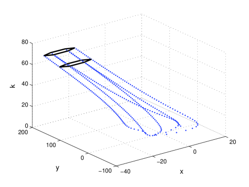
Figure 4. The agents form a regular hexagon.

7. Conclusions

This paper has studied the consensus of discrete-time multi-agent systems with linear or linearized dynamics. An observer-type protocol based on the relative outputs of neighboring agents has been proposed, which can be seen as an extension of the traditional observer-based controller for a single system to one for multi-agent systems. The consensus of high-dimensional multi-agent systems with directed communication topologies can be converted into the stability of a set of matrices with the same low dimension as that of a single agent. The notion of discrete-time consensus region has been introduced and analyzed. For neurally stable agents, an algorithm has been presented to construct a protocol having a bounded consensus region in the form of the open unit disk. Moreover, for unstable agents, another algorithm has also been proposed to construct a protocol having an origin-centered disk of radius $\delta$ ($0<\delta<1$) as its consensus region. The consensus algorithms have been further applied to solve formation control problems of multi-agent systems. To some extent, this paper generalizes some existing results reported in the literature, and opens up a new line for further research on discrete-time multi-agent systems.

Received xxxx 20xx; revised xxxx 20xx.

References

- [1] D. Bauso, L. Giarré and R. Pesenti, Consensus for netowrks with unknown but bounded disturbances, SIAM J. Control Optim., 48 (2009), 1756–1770.
- [2] S. Bowong and J. L. Dimi, Adaptive synchronization of a class of uncertain chaotic systems, Discret. Contin. Dyn. Syst., 9 2008, 235–248.
- [3] J. Corts, Distributed algorithms for reaching consensus on general functions, Automatica, 44 (2008), 726–737.
- [4] Z. S. Duan, G. R. Chen and L. Huang, Synchronization of weighted networks and complex synchronized regions, Phys. Lett. A, 372 (2008), 3741–3751.
- [5] Z. S. Duan, G. R. Chen, and L. Huang, Disconnected synchronized regions of complex dynamical networks, IEEE Trans. Autom. Control, 54 (2009), 845–849.
- [6] J. A. Fax and R. M. Murray, Information flow and cooperative control of vehicle formations, IEEE Trans. Automat. Control, 49 (2004), 1465–1476.
- [7] P. Frasca, R. Carli, F. Pagnani and S. Zampieri, Average consensus on networks with quantized communication, Int. J. Robust Nonlinear Control, 19 (2008), 1787–1816.
- [8] Y. Hong, J. Hu and L. Gao, Tracking control for multi-agent consensus with an active leader and variable topology, Automatica, 42 (2006), 1177–1182.
- [9] Y. Hong, G. R. Chen and L. Bushnell, Distributed observers design for leader-following control of multi-agent, Automatica, 44 (2008), 846–850.
- [10] R. Horn and C. Johnson, “Matrix Analysis,” Cambridge Univ. Press, New York, 1985.
- [11] A. Jadbabaie, J. Lin and A. S. Morse, Coordination of groups of mobile autonous agents using neareast neighbor rules, IEEE Trans. Autom. Control, 48 (2003), 988–1001.
- [12] T. Katayama, On the matrix Riccati equation for linear systems with a random gain, IEEE Trans. Autom. Control, 21 (1976), 770–771.
- [13] G. Lafferriere, A. Williams, J. Caughman and J. J. P. Veerman, Decentralized control of vehicle formations, Syst. Control Lett., 54 (2005), 899–910.
- [14] Z. K. Li, Z. S. Duan and L. Huang, control of networked multi-agent systems, J. Syst. Sci. Complex., 22 2009, 35–48.
- [15] Z. K. Li, Z. S. Duan, G. R. Chen and L. Huang, Consensus of multiagent systems and synchronization of complex networks: A unified viewpoint, IEEE Trans. Circuits Syst. I-Regul. Pap., 51 (2010), 213–224.
- [16] Z. K. Li, Z. S. Duan and G. R. Chen, Dynamic consensus of linear multi-agent systems, IET Control Theory Appl., 5 (2011), 19–28.
- [17] P. Lin, Y. M. Jia and L. Li, Distributed robust consensus control in directed networks of agents with time-delay, Syst. Control Lett., 57 (2008), 643–653.
- [18] P. Lin and Y. M. Jia, Further results on decentralised coordination in networks of agents with second-order dynamics, IET Control Theory Appl., 3 (2009), 957–970.
- [19] C. Liu, Z. S. Duan, G. R. Chen and L. Huang, Analyzing and controlling the network synchronization regions, Physica A, 386 (2007), 531–542.
- [20] C. Q. Ma and J. F. Zhang, Necessary and sufficient conditions for consensusability of linear multi-agent systems, IEEE Trans. Autom. Control, 55 (2010), 1263–1268.
- [21] K. Ogata, “Modern Control Engineering,” 3rd edition, Prentice Hall: Englewood Cliffs, 1996.
- [22] R. Olfati-Saber and R. M. Murray, Consensus problems in networks of agents with switching topology and time-delays, IEEE Trans. Autom. Control, 49 (2004), 1520–1533.
- [23] R. Olfati-Saber, Flocking for multi-agent dynamic systems: Algorithms and theory, IEEE Trans. Autom. Control, 51 (2006), 401–420.
- [24] R. Olfati-Saber, J. A. Fax and R. M. Murray, Consensus and cooperation in networked multi-agent systems, Pro. IEEE, 97 (2007), 215–233.
- [25] L. M. Pecora and T. L. Carroll, Master stability functions for synchronized coupled systems, Phys. Rev. Lett., 80 (1998), 2109–2112.
- [26] W. Ren and R. W. Beard, consensus seeking in multiagent systems under dynamically changing interaction topogies, IEEE Trans. Autom. Control, 50 (2005), 655–661.
- [27] W. Ren, R. W. Beard and E. M. Atkins, Information consensus in multivehicle cooperative control, IEEE Control Syst. Mag., 27 (2007), 71–82.
- [28] W. Ren, K. L. Moore and Y. Q. Chen, High-order and model reference consensus algorithms in cooperative control of multi-vehicle systems, J. Dyn. Syst. Meas. Control-Trans. ASME, 129 (2007), 678–688.
- [29] W. Ren, On consensus algorithms for double-integrator dynamics, IEEE Trans. Autom. Control, 53 (2008), 1503–1509.
- [30] W. Ren and N. Sorensen, Distributed coordination architecture for multi-robot formation control, Robot. Auton. Syst., 56 (2008), 324–333.
- [31] A. Rahmani, M. Ji, M. Mesbahi and M. Egerstedt, Controllability of multi-agent systems from a graph-theorectic perspective, SIAM J. Control Optim., 48 (2009), 162–186.
- [32] L. Scardavi and S. Sepulchre, Synchronization in networks of identical linear systems, Automatica, 45 (2009), 2557–2562.
- [33] L. Schenato,B. Sinopoli,M. Franceschetti, K. Poolla, M. I. Jordan and S. S. Sastry, Foundations of control and estimation over lossy networks, Proc. IEEE, 95 (2007), 163–187.
- [34] J. H. Seo, H. Shim and J. Back, Consensus of high-order linear systems using dynamic output feedback compensator: Low gain approach, Automatica, 45 (2009), 2659–2664.
- [35] B. Sinopoli, L. Schenato, M. Franceschetti, K. Poolla, M. I. Jordan and S. S. Sastry, Kalman filtering with intermittent observations, IEEE Trans. Autom. Control, 49 (2004), 1453–1464.
- [36] Y. G. Sun and W. Long, Consensus problems in networks of agents with double-integrator dynamics and time-varying delays, Int. J. Control, 82 (2009), 1937–1945.
- [37] R. S. Smith and F. Y. Hadaegh, Control of deep-space formation-flying spacecraft; Relative sensing and switched information, J. Guid. Control Dyn., 28 (2005), 106–114.
- [38] H. S. Su. X. F. Wang Z. L. Lin, Flocking of multi-agents with a virtual leader, IEEE Trans. Autom. Control, 54 (2009), 293–307.
- [39] H. G. Tanner, A. Jadbabaie and G. J. Pappas, Flocking in fixed ans switching networks, IEEE Trans. Autom. Control, 52 (2007), 863–868.
- [40] Y. P. Tian and C. L. Liu, Robust consensus of multi-agent systems with diverse input delays and asymmetric interconnection perturbations, Automatica, 45 (2009), 1347–1353.
- [41] S. E. Tuna, Synchronizing linear systems via partial-state coupling, Automatica, 44 (2008), 2179–2184.
- [42] S. E. Tuna, Conditions for synchronizability in arrays of coupled linear systems, IEEE Trans. Autom. Control, 54 (2009), 2416–2420.
- [43] T. Vicsek, A. Cziroók, E. Ben-Jacob, I. Cohen and O. Shochet, Novel type of phase transitions in a system of self-driven particles, Phys. Rev. Lett., 75 (1995), 1226–1229.
- [44] J. H. Wang, D. Z. Cheng and X. M. Hu, Consensus of multi-agent linear dynamic systems, Asian J. Control, 10 (2008), 144–155.
- [45] G. Xie and L. Wang, Consensus control for a class of networks of dynamic agents, Int. J. Robust Nonlinear Control, 17 (2007), 941–959.
- [46] R. Yamapi and R. S. Mackay, Stability of synchronization in a shift-invariant ring of mutually coupled oscillators, Discret. Contin. Dyn. Syst., 10 (2008), 973–996.
- [47] H. T. Zhang, M. Z. Q. Chen, T. Zhou and G. B. Stan, Ultrafast consensus via predictive mechanisms, Europhysics Letters, 83 (2008), 40003.
- [48] K. M. Zhou and J. C. Doyle, “Essentials of Robust Control,” Prentice-Hall, Englewood Cliffs, 1998.