Low Complexity Kolmogorov-Smirnov Modulation Classification
Abstract
Kolmogorov-Smirnov (K-S) test–a non-parametric method to measure the goodness of fit, is applied for automatic modulation classification (AMC) in this paper. The basic procedure involves computing the empirical cumulative distribution function (ECDF) of some decision statistic derived from the received signal, and comparing it with the CDFs of the signal under each candidate modulation format. The K-S-based modulation classifier is first developed for AWGN channel, then it is applied to OFDM-SDMA systems to cancel multiuser interference. Regarding the complexity issue of K-S modulation classification, we propose a low-complexity method based on the robustness of the K-S classifier. Extensive simulation results demonstrate that compared with the traditional cumulant-based classifiers, the proposed K-S classifier offers superior classification performance and requires less number of signal samples (thus is fast).
Index Terms:
Automatic modulation classification, Kolmogorov-Smirnov test, OFDM, interference cancellation.I Introduction
Automatic modulation classification is a procedure performed at the receiver based on the received signal before demodulation when the modulation format is not known to the receiver. It plays a key role in various tactical communication applications. It also finds applications in emerging wireless communication systems that employ interference cancellation techniques – in order to demodulate and cancel the unknown interfering user’s signal, its modulation format needs to be classified first.
The feature-based modulation classification methods are popular, and they base on feature extraction and decision [1]-[5]. The most widely used feature is the cumulant. It can be used to classify many different modulation types by high-order statistic cumulants [4]. It is simple to implement and can achieve nearly optimal performance with large number of samples [6]. For example, the fourth-order cumulant can be used to classify various low-order modulations. For classifying higher-order constellations, a higher-order cumulant is needed. An accurate estimate of the higher-order cumulant of the signal requires a large number of signal samples. Most of the existing works on modulation classification focus on the additive white Gaussian noise (AWGN) channel. A few works have considered fading and multipath channels [6], [7]. However, effective modulation classifier with less signal samples remains a challenge.
In this paper, we propose to employ the Kolmogorov-Smirnov (K-S) test [8] for modulation classification. The K-S test is a non-parametric statistical method to measure the goodness of fit. From the received signal, we compute the empirical cumulative distribution function (CDF) of certain decision statistic. A priori we also compute the CDF of the same decision statistic under each candidate modulation format. The modulation format that results in the minimum of the maximum distance between its CDF and the observed empirical CDF is the final decision. We develop K-S classifiers based on quadrature amplitude decision statistics, then apply it to OFDM-SDMA systems to cancel the multiuser interference. Regarding high complexity involved by CDF calculation, we propose a low-complexity method based on the robustness of K-S classifier111It is worth to point out that during the preparation of this paper’s presentation we discover the impressive work in [9] that was submitted recently and investigates low complexity issue of modulation classification.. We provide extensive simulation results to demonstrate the performance gain of the proposed K-S classifiers over the cumulant-based classifiers. The remainder of this paper is organized as follows. In Section II we provide some background on modulation classification and on the K-S test. In Section III, we develop the K-S-based modulation classifiers based on K-S test, and its corresponding low-complexity method. Section IV is devoted to an application of K-S classifier in OFDM-SDMA system for interference signal recognition and cancellation. Simulation results are provided in Section V. Section VI concludes the paper.
II Background
II-A Automatic Modulation Classification
Consider the following discrete-time additive white noise channel model
| (1) |
where , and are respectively the complex-valued transmitted modulation symbol, the received signal, and the noise sample at time . The transmitted symbols are drawn from an unknown constellation set which in turn belongs to a set of possible modulation formats . The modulation classification problem refers to the determination of the constellation set to which the transmitted symbols belong based on the received signals . There are two major approaches in the literature to solving the above modulation classification problem. In the likelihood-based methods [10], [11], some form of the likelihood for each modulation format is calculated by making certain assumption on the data sequence. The classification decision then corresponds to the modulation with the largest likelihood value. These methods are typically computationally very expensive. Moreover, they require the knowledge of the various channel parameters and become ineffective in the presence of unknown channel impairment such as fading, phase and frequency offsets, and non-Gaussian interference/noise.
The more popular and low-complexity approach to automatic modulation classification is based on cumulant [4], [6]. Specifically, for the system given by (1), we calculate the normalized sample fourth-order cumulant of the received signal as
| (2) |
The modulation whose theoretical cumulant [10] is closest to is then the classification decision. The fourth-order cumulants can be used to classify 4-QAM, 16-QAM and 64-QAM modulations. For even higher-order modulations, the difference between the cumulants becomes small, which leads to low classification accuracy. A higher-order cumulant should be used to classify these modulations, with a considerably increased computational complexity.
II-B Kolmogorov-Smirnov (K-S) Test
The Kolmogorov-Smirnov (K-S) test is a non-parametric test of goodness of fit for the continuous cumulative distribution of the data samples [8], [12], [13]. It can be used to approve the null hypothesis that two data populations are drawn from the same distribution to a certain required level of significance. On the other hand, failing to approve the null hypothesis shows that they are from different distributions.
In this paper we consider the one sample K-S test. In the test, we are given a sequence of i.i.d. real-valued data samples with the underlying cumulative distribution function (CDF) , and a hypothesized distribution with the CDF . The null hypothesis to be tested is
| (3) |
The K-S test first forms the empirical CDF from the data samples
| (4) |
where is the indicator function, which equals to one if the input is true, equals to zero otherwise. The largest absolute difference between the two CDF’s is used as the goodness-of-fit statistic, given by
| (5) |
and in practical, it is calculated by
| (6) |
The significance level of the observed value is given by
| (7) | ||||
| (8) |
The hypothesis is rejected at a significance level if .
III K-S-based Modulation Classification
Consider the signal model in (1). In this section, we assume that the i.i.d. noise samples follow the complex Gaussian distribution, i.e., ; that is, the real and imaginary components of are independent and have the same Gaussian distribution . To classify the modulation based on the received signals using the K-S test, we first form a sequence of decision statistics from , where can be either the magnitude, or the phase, or the real and imaginary components of , and then compute the corresponding empirical CDF . In the meantime, for each possible modulation candidate , we can obtain either the CDF for . The K-S statistic is then calculated by
| (9) |
The decision on the modulation is given by the minimum K-S statistic, i.e.,
| (10) |
Moreover, recall that associated with each K-S statistic , there is a significance level , computed by (7). The normalized can be used to give a “soft” decision on the modulation, that is, the probability that the modulation is used approximately . In what follows, we discuss the decision statistics for different modulation formats, and the corresponding CDF .
We consider the quadrature amplitude modulation (QAM) formats, e.g., 4-QAM, 16-QAM, and 64-QAM. The set of signal points of unit-energy constellations for these modulations are given by , , , where .
We suggest a quadrature-based K-S classifier, which is first proposed in our work of [14]. Since for QAM input signals, the real and imaginary components of the received signal are independent and have identical distributions, we can also use them directly as the decision statistics. That is, from the received signals samples , we form a sequence of samples of decision statistic
Then we have . Hence the CDF under modulation is given by
| (11) |
where is Gaussian Q-function, and denotes the set of real components of the signal points in . The K-S test in (9)-(10) can be performed using and on the samples .
Due to the complicated CDF expressions, it is computationally expensive to calculate CDF at each samples. Since the K-S classifier has the property of robustness, which will be proved in Fig. 1, i.e. the correct classification performance is robust to SNR mismatch. With respect to the robustness, we can quantize the received SNR with different granularity. In a certain quantization, one CDF curve is stored for each SNR, where the curves are also comprising of discrete points which are denser than the SNR interval. All the curves can be computed offline. With the storage of these CDF curves, we can avoid the complicated computation by looking up tables. Thus, all involved computations are only ECDF calculation and comparison operation.
IV Application: Interference Cancellation in OFDM-SDMA Systems
We next consider an application of modulation classification in the context of interference cancellation in an OFDM system employing multiple receive antennas. Specifically, assuming the OFDM receiver is equipped with two receive antennas, which makes it possible to have two users simultaneously transmitting data – the so-called space-division multiple-access (SDMA) [15]. That is, the received signal at the -subcarrier of the -th OFDM word is given by
| (12) |
where denotes the received signals at the two receive antennas; denotes the channels between the desired user’s transmitter and the receive antennas; denotes the channels between the interfering user’s transmitter and the receive antennas; is the received noise sample vector.
The receiver aims to demodulate the desired user’s symbols . It is assumed that the receiver knows the modulation of the desired user, but not that of the interferer. It is also assumed that the receiver can estimate the channels of both the desired user and the interferer, . A simple receiver scheme is to apply a linear MMSE filter to the received signal to suppress the interferer, and demodulate based on the output of this filter. A more powerful receiver scheme is to employ interference cancellation. That is, we first demodulate the interferer’s symbols and then subtract the interferer’s signals from the received signals. Finally we demodulate the desired user’s symbols based on the post-cancellation signals. In order to estimate the interferer’s symbols, we must first classify the modulation format used by the interferer. Hence the interference cancellation receiver consists of the follow steps.
-
•
For each subcarrier, apply a linear MMSE filter to the received signal to suppress the desired signal
(13) By the choice of in (37), we can write
(14) where contains the residual desired user’s signal and noise. The distribution of can be accurately modeled as Gaussian with zero mean and variance .
- •
-
•
Once the modulation format of the interferer on each subcarrier group is estimated, we can demodulate the interferer’s symbols based on the linear MMSE filter output (14).
-
•
Next we perform interference cancellation on each subcarrier, followed by a matched-filtering for the desired users’s signals, i.e.,
(15) Finally the desired user’s symbol is demodulated from .
V Simulation Results
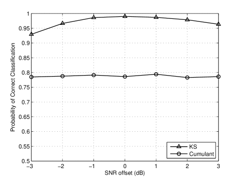
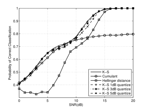
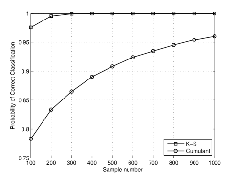
In this section, we provide simulation results to compare the performance of the proposed K-S-based modulation classifier with that of the cumulant-based one. For the QAM modulations, we will consider the set 4-QAM, 16-QAM, 64-QAM in AWGN channel. The channel model is given by (1) with . The signal-to-noise ratio (SNR) is defined as . The 4-th order cumulants are used. The number of received signal samples used is = 100. In Fig. 1, consider the SNR mismatch at the receiver. If the noise power is half or twice as the original value, there is 3dB or -3dB SNR mismatch. We compare the robustness of K-S and cumulant classifiers. In the whole range, K-S classifier is always much better than the cumulant one, although there is degradation on large value of SNR offset. Cumulant method is robust in the range, however, its performance is not satisfactory with such few sample number. The classification performance of various classifiers in AWGN channels for QAM modulations is shown in Fig. 2, including quantized K-S classifier. We also show the performance of the Hellinger-distance-based classifier [16] which has a very high complexity. It is seen that for such a small sample size, at high SNR, the cumulant-based methods exhibit a ceiling on the classification probability around 0.8. However, the K-S-based classifier monotonically improves the classification performance as the SNR increases and it significantly outperforms the cumulant-based classifier at high SNR. The Hellinger-distance-based classifier performs worse than the cumulant method in the low SNR region and in the high SNR region it performs worse than the K-S quadrature method. As is shown in Fig. 2, the performance suffers more as the SNR quantized interval increases, where the quantized interval of each CDF curve is 0.01 and the scale is between -4 to 4, and larger values are ignored since they are with trivial probability. With respect to the performance degradation at -3dB and 3dB SNR mismatch in Fig. 1, K-S classifier is still superior to the other two classifiers even with 5dB quantized interval. The classification performance for QAM modulations as a function of the sample size is shown in Fig. 3.
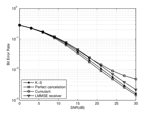
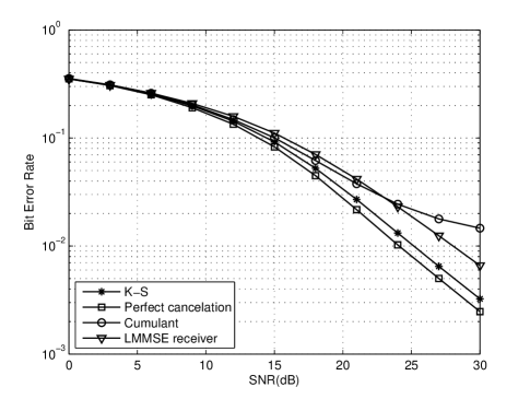
We next consider the effect of modulation classification on the performance of interference cancellation in an OFDM system employing multiple receive antennas. The signal model is given by (12). Again the 3GPP channel model is used to generate the multipath channels for multiple antennas [17], [18]. There are 512 subcarriers in one OFDM symbol, which are shared by both the desired user and the interferer. For simplicity we assume that the same QAM modulation is employed on all subcarriers for each user. Hence modulation classification is based on samples from one OFDM symbol. We assume that the channels of both the desired user and the interferer are known. In Fig. 4 and Fig. 5 we compare the bit error rate (BER) performance of four receivers, namely, the linear MMSE receiver, the interference cancellation receivers using the K-S modulation classifier and the cumulant-based modulation classifier, respectively, and an “ideal” receiver that is assumed capable of completely removing the interferer’s signal (and hence achieving single-user performance.) Note that the last receiver performance serves as a lower bound to the performance of any practical receiver. In Fig. 4 the desired user employs 16-QAM whereas in Fig. 5 the desired user employs 64-QAM. It is seen that performance of the receiver that uses the cumulant-based classifier is even worse than that of the linear MMSE receiver. This is because even with a sample size of 512, the cumulant-based classifier has a relatively low accuracy in detecting the modulation and with the wrong modulation information, the interference cancellation receiver actually enhances the interference. On the other hand, the receiver that employs the K-S classifier exhibits performance that is close to the ideal receiver performance, and offer a gain of 2dB and 3dB respectively at the BER of 0.01 compared to the linear MMSE receiver.
VI Conclusion
We have proposed a new modulation classification technique based on the Kolmogorov-Smirnov (K-S) test, for classifying different QAM modulation formats. The basic procedure involves computing the ECDF of some decision statistic derived from the received signal, and comparing it with the CDFs of the signal under each candidate modulation format. Compared with the popular cumulant-based modulation classifiers, the proposed K-S classifiers offer faster (i.e., requiring less number of signal samples) and superior performance. Regarding the complexity issue, we propose the low complexity method based on the robustness of K-S classifier. Moreover, the K-S classifier offers a method of interference cancellation in OFDM-SDMA systems.
Acknowledgment
This work is supported by Program for Changjiang Scholars and Innovative Research Team in University under Grant No. IRT0949; the Joint Funds of State Key Program of NSFC (Grant No. 60830001); Program for New Century Excellent Talents in University under Grant NCET-09-0206; the Key Project of State Key Lab. of Rail Traffic Control and Safety under Grant RCS2008ZZ006 and RCS2008ZZ007.
References
- [1] S. Soliman and S.-Z. Hsue, “Signal classification using statistical moments,” Communications, IEEE Transactions on, vol. 40, no. 5, pp. 908–916, 1992.
- [2] Y. Yang and C.-H. Liu, “An asymptotic optimal algorithm for modulation classification,” Communications Letters, IEEE, vol. 2, no. 5, pp. 117–119, 1998.
- [3] P. Marchand, J.-L. Lacoume, and C. Le Martret, “Multiple hypothesis modulation classification based on cyclic cumulants of different orders,” in Acoustics, Speech and Signal Processing, 1998. Proceedings of the 1998 IEEE International Conference on, vol. 4, Seattle, WA, USA, 1998, pp. 2157–2160.
- [4] A. Swami and B. Sadler, “Hierarchical digital modulation classification using cumulants,” Communications, IEEE Transactions on, vol. 48, no. 3, pp. 416–429, 2000.
- [5] W. Dai, Y. Wang, and J. Wang, “Joint power estimation and modulation classification using second- and higher statistics,” in Wireless Communications and Networking Conference, 2002. WCNC2002, IEEE, vol. 1, 2002, pp. 155–158.
- [6] H.-C. Wu, M. Saquib, and Z. Yun, “Novel automatic modulation classification using cumulant features for communications via multipath channels,” Wireless Communications, IEEE Transactions on, vol. 7, no. 8, pp. 3098–3105, 2008.
- [7] A. Swami, S. Barbarossa, and B. Sadler, “Blind source separation and signal classification,” in Signals, Systems and Computers, 2000. Conference Record of the Thirty-Fourth Asilomar Conference on, vol. 2, Pacific Grove, CA, USA, 2000, pp. 1187–1191.
- [8] F. Massey, “The Kolmogorov-Smirnov test for goodnees of fit,” Journal of the American Statistical Association, vol. 46, no. 256, pp. 68–78, 1951.
- [9] P. Urriza, E. Rebeiz, P. Pawelczak, and D. Cabric, “Computationally efficient modulation level classification based on probability distribution distance functions,” CoRR, vol. abs/1012.5327, 2010.
- [10] O. Dobre, A. Abdi, Y. Bar-Ness, and W. Su, “Survey of automatic modulation classification techniques: classical approaches and new trends,” Communications, IET, vol. 1, no. 2, pp. 137–156, 2007.
- [11] W. Wei and J. Mendel, “Maximum-likelihood classification for digital amplitude-phase modulations,” Communications, IEEE Transactions on, vol. 48, no. 2, pp. 189 – 193, 2000.
- [12] W. Conover, Practical Nonparametric Statistics. John Wiley and Sons, 1980.
- [13] W. Press, Numerical Recipes in C. Cambridge University Press, 1992.
- [14] F. Wang, X. Wang, and W. Wang, “Fast and robust modulation classification via Kolmogorov-Smirnov test,” Communications, IEEE Transactions on, vol. 58, no. 8, pp. 2324 – 2332, Aug 2010.
- [15] G. Boudreau, J. Panicker, N. Guo, R. Chang, N. Wang, and S. Vrzic, “Interference coordination and cancellation for 4G networks,” IEEE Communications Magazine, vol. 47, no. 4, pp. 74–81, 2009.
- [16] X. Huo and D. Donoho, “A simple and robust modulation classification method via counting,” in Acoustics, Speech and Signal Processing, 1998. Proceedings of the 1998 IEEE International Conference on, 1998, pp. 3289–3292.
- [17] “MATLAB implementation of the 3GPP spatial channel model (3GPP TR 25.996),” http://www.tkk.fi/Units/Radio/scm/, Jan. 2005.
- [18] “Spatial channel model for multiple input multiple output (MIMO) simulations, 3GPP TR 25.996 V8.0.0,” http://www.3gpp.org, Dec. 2008.