The solution of the quantum $A_{1}$ $T$-system for arbitrary boundary

Abstract.

We solve the quantum version of the $A_{1}$ $T$-system by use of quantum networks. The system is interpreted as a particular set of mutations of a suitable (infinite-rank) quantum cluster algebra, and Laurent positivity follows from our solution. As an application we re-derive the corresponding quantum network solution to the quantum $A_{1}$ $Q$-system and generalize it to the fully non-commutative case. We give the relation between the quantum $T$-system and the quantum lattice Liouville equation, which is the quantized $Y$-system.

1. Introduction

The $T$-systems [18, 21] satisfied by the transfer matrices of the generalized Heisenberg model or the $q$-characters of quantum affine algebras [16] can be considered as discrete dynamical systems with special initial conditions. More generally, the equations of these systems can be shown [6] to be mutations in an infinite-rank cluster algebra [13]. As such, their solutions under general boundary conditions [8, 5] are expected to satisfy special properties such as the Laurent property and positivity.

Among discrete dynamical systems, the cluster algebras of Fomin and Zelevinsky [13] hold a special place. These describe the evolution of data vectors (clusters) attached to the nodes of an infinite regular tree via mutations along the edges. Mutations are defined in such a way that the following Laurent property is guaranteed: any cluster data may be expressed as a Laurent polynomial of the cluster variables at any node of the tree. It was conjectured in [13] and proved in several particular cases (in particular in the so-called acyclic cases [3, 15, 1], or that of clusters arising from surfaces [22]) that these polynomials always have non-negative integer coefficients (Laurent positivity), a property that still awaits a good general combinatorial interpretation.

Cluster algebras turn out to be quite universal, and have found applications in various fields, such as the study of non-linear recursions, the geometry of Teichmüller space, quiver representations, wall crossing formulas etc.

The relation between the recursion satisfied by the ($q$-) characters of KR-modules of quantum affine algebras on the one hand, and cluster algebras on the other, was found in [17, 6]. Such systems are known as $Q$-sytems or $T$-systems when they are supplemented by special boundary conditions. It is known that such equations can be interpreted as discrete integrable systems: In the case of an $A_{r}$ type algebra, the $T$-system was identified as the discrete Hirota equation [20]. It is also known as the tetrahedron equation in combinatorics, and arises in the context of the Littlewood-Richardson coefficients for tensor products of irreducible representations of $A_{r}$ [19] and domino tilings of the Aztec diamond [23].

Solutions to the $Q$ and $T$-systems have been constructed by various authors [20]. Recently, a transfer matrix solution was given for the $A_{1}$ $T$-system in the case of arbitrary boundary conditions. The latter is also known in the combinatorics literature as frieze equation [1]. This solution was generalized to the case of $A_{r}$ in [5]. It amounts to representing general solutions of the system as partition functions for paths on a positively weighted graph or network. The graph is determined solely by the initial conditions.

The connection to cluster algebras is as follows [17, 6]: One shows that the admissible initial data for the $T$-systems form a subset of the clusters a cluster algebra, and that the mutations in this algebra are local transformations which are the $T$-system equations. Thus the expression of the solutions as partition functions for positively weighted paths implies the Laurent positivity for these particular clusters.

An important question is how to quantize such evolution equations [11, 12]. The quantization in the case of cluster algebras generally was given by Berenstein and Zelevinsky [2]. Quantum cluster algebras are non-commutative algebras where the cluster variables obey special commutation relations depending on a deformation parameter $q$. Mutations are defined in such a way that the Laurent property is preserved, and a positivity conjecture is also expected to hold: That is, any cluster variable may be expressed as a Laurent polynomial of the variables in any other cluster seed, with coefficients in ${\mathbb{Z}}_{+}[q,q^{-1}]$. Quantum cluster algebras were used in [10] to define quantum $Q$-systems for $A_{r}$.

In the present paper, we focus on the $T$ system for $A_{1}$, and construct its quantum version via the cluster algebra connection. We gather a few definitions in Section 2 and construct the quantum $A_{1}$ $T$-system in Section 3. We then express the general solution in Section 4 by use of a non-commutative transfer matrix, quantizing the solution of [5]. The main result of the paper is Theorem 4.4, which implies an interpretation of the solution as a partition function for “quantum paths” with step weights which are non-commutative Laurent monomials in the initial data, thereby proving Laurent positivity for the relevant clusters.

The $2$-periodic solutions of the $T$-systems satisfy $Q$-system equations, and this generalizes to the quantum case. The $A_{1}$ $Q$-system has a fully non-commutative generalization introduced by Kontsevich in the framework of wall-crossing phenomena in non-commutative Donaldson-Thomas invariant theory. The solution was given in [9] for this system using the method of [7]. We revisit this system in Section 5 and formulate a fully non-commutative (as opposed to $q$-commutative) version of the network transfer matrices used in Section 4 to solve the $T$-system. This gives an alternative solution for the non-commutative $A_{1}$ $Q$-system.

Finally in Section 6 we give the relation between the quantum $A_{1}$ $T$-system and the discrete quantum Liouville equation of Faddeev et al [11, 12]. This equation can also be viewed as a non-commutative $Y$-system.

Acknowledgments. We thank L. Faddev for illuminating remarks, and the organizers of the MSRI semester program on “Random Matrix Theory, Interacting Particle Systems and Integrable Systems” where this work was completed. PDF received partial support from the ANR Grant GranMa. The work of RK is supported by NSF grant DMS-0802511.

2. Definitions

2.1. Cluster algebras and quantum cluster algebras

We use a simplified version of the definition of Fomin and Zelevinsky [13] of cluster algebras of geometric type with trivial coefficients.

2.1.1. Cluster algebras of geometric type

A cluster algebra is the commutative ring generated by the union of commutative variables called cluster variables. The generators are related by rational transformations called mutations determined by an exchange matrix, which governs the discrete dynamics of the system.

For the purposes of his paper, it is sufficient to consider a cluster algebra of rank $n$, with a seed cluster consisting of $n$ cluster variables ${\mathbf{x}}=(x_{1},...,x_{n})$ and an $n\times n$ skew-symmetric exchange matrix $B$. (We will also have occasion to consider cluster algebras of infinite rank ($n\to\infty$). It will be clear from our solution that when such algebras occur they are well-defined as a completion of the finite rank case.)

Clusters are pairs $({\mathbf{x}}(t),B(t))$ where $t$ is a label of a node of a complete $n$-tree. Each node is associated with a cluster. The edges of the tree are labeled in such a way that each node is connected to exactly one edge with label $k$ where $k\in[1,...,n]$.

The clusters at nodes $t$ and $t^{\prime}$ connected by an edge labeled $k$ are related to each other by a mutation, which acts as a rational transformation on the component $x_{k}(t)$: ${\mathbf{x}}(t^{\prime})=\mu_{k}({\mathbf{x}}(t))$ where

(2.1) $$x_{j}(t^{\prime})=\left\{\begin{array}[]{ll}x_{j}(t),&k\neq j,\\ (x_{k}(t))^{-1}\left(\displaystyle{\prod_{B_{j,k}>0}x_{j}(t)^{B_{j,k}}+\prod_{B_{j,k}<0}x_{j}(t)^{-B_{j,k}}}\right),&k=j.\end{array}\right.$$

A mutation also acts on the exchange matrix $B(t)$, such that $B(t^{\prime})=\mu_{k}(B(t))$ if $t$ and $t^{\prime}$ are connected by an edge labeled $k$, and

(2.2) $$B_{i,j}(t^{\prime})=\left\{\begin{array}[]{ll}-B_{i,j}(t)&\hbox{if $i=k$ or $j=k$, }\\ B_{i,j}(t)+{\rm sign}(B_{i,k}(t))[B_{i,k}(t)B_{k,j}(t)]_{+}&\hbox{otherwise}.\end{array}\right.$$

with the notation $[x]_{+}={\rm Max}(x,0)$. To define a cluster algebra, it is sufficient to give the seed $({\mathbf{x}},B)$ at one single node. This then determines the cluster variables at all other nodes via iterated mutations.

2.1.2. Quantum cluster algebras

It is interesting to consider whether there exist non-commutative generalizations of cluster algebras, which maintain some of the properties of cluster algebras. In particular, the Laurent property [14] and the (conjectured in general) positivity of a cluster variable at any node as an expression in terms of the cluster variables at any other node. We considered some possible candidates in [10] motivated by our consideration of the integrable subcluster algebras described by $Q$-systems and $T$-systems, as well as the Kontsevich wall-crossing formula. We also considered the specialization of these non-commutative systems to the simplest type of non-commutativity, the $q$-deformation. Such systems were first considered by Berenstein and Zelevinsky in Ref.[2], where they defined “quantum cluster algebras”. We give here a simplified version of their definition which is sufficient for this paper.

A quantum cluster algebra is the skew field of rational functions generated by the non-commutative cluster variables $\{{\mathbf{X}}(t)=(X_{1}(t),...,X_{n}(t))\}$ where $t$ are the labels of the complete $n$-tree as above. At a node $t$ we have the cluster $({\mathbf{X}},B):=({\mathbf{X}}(t),B(t))$ where the exchange matrix is the same as for the usual cluster algebra. The cluster variables at this node $q$-commute:

(2.3) $$X_{i}X_{j}=q^{\lambda_{ij}}X_{j}X_{i}.$$

Here $\lambda_{ij}$ are the entries of an $n\times n$ skew-symmetric matrix $\Lambda$. Up to a scalar multiple, we can take $\Lambda$ to be the inverse of the exchange matrix $B$. According to the definitions of [13] such a matrix $\Lambda$ is “compatible” with the exchange matrix $B$.

Equivalently, we can define $X_{j}=e^{a_{j}}$, where $a_{j}$ are also non-commuting variables and the exponential is taken formally. Then the commutation relations above correspond to $[a_{i},a_{j}]=h\lambda_{i,j}$ where $q=e^{h}$.

Clusters at tree nodes $t$ and $t^{\prime}$ connected by an edge labeled $k$ are related by a mutation. Let ${\mathbf{X}}^{\boldsymbol{\alpha}}={\rm exp}(\sum_{j}\alpha_{j}a_{j})$. Then we define ${\mathbf{X}}(t^{\prime})=\mu_{k}({\mathbf{X}}(t))$ to be

(2.4) $$X_{j}(t^{\prime})=\left\{\begin{array}[]{ll}X_{j}(t)&\hbox{if $j\neq k$};\\ {\mathbf{X}}^{-e_{k}+\sum_{i}[B_{ik}]_{+}e_{i}}+{\mathbf{X}}^{-e_{k}+\sum_{i}[-B_{ik}]_{+}e_{i}}&j=k.\end{array}\right.$$

The exchange matrix $B(t^{\prime})=\mu_{k}(B(t))$ is the same as in the commutative case.

2.2. The $A_{1}$ $T$-system

The $T$-systems appear in the solution of exactly solvable models in statistical mechanics, in the Bethe ansatz of generalized Heisenberg quantum spin chains based on representations of Yangians of each simple Lie algebra [18, 21]. The transfer matrices of the model satisfy a recursion relation in the highest ${\mathfrak{g}}$-weight of the $Y({\mathfrak{g}})$-modules corresponding to the auxiliary space. These relations are called $T$-systems. In the context of representation theory, these relations are the equations satisfied by the $q$-characters [16] of Kirillov-Reshetikhin modules of the Yangians, or the associated quantum affine algebra.

2.2.1. The $T$-system associated to $A_{1}$

These systems provide examples of discrete integrable systems which are part of a suitable cluster algebra structure [6]. However, in the representation-theoretical context, a special initial condition is placed on the variables (corresponding to the fact that the $q$-character of the trivial representation is 1). Here, we dispense with this special value. Moreover, we renormalize the variables so that the solutions are positive Laurent polynomials of the initial data for any initial data. This corresponds to normalizing the cluster variables of the cluster algebras so that all coefficients are trivial.

Thus, with slight abuse of notation, we call the following system the $A_{1}$ $T$-system:

(2.5) $$T_{i,j+1}T_{i,j-1}=T_{i+1,j}T_{i-1,j}+1\qquad(i,j\in{\mathbb{Z}}).$$

Here, we consider the set $\{T_{i,j}|i,j\in{\mathbb{Z}}\}$ as commutative variables. Solutions of the equation are given as functions of a choice of initial variables.

Remark 2.1.

Upon a simple change of coordinates, this system is also known as “frieze” equation in combinatorics [4, 1].

2.2.2. Initial conditions

Equations (2.5) split into two independent sets of recursion relations, since the parity of $i+j$ is preserved by the equations. Without loss of generality, let us restrict to the relations for $\{T_{i,j}|i,j\in{\mathbb{Z}},\ i+j\equiv 0\!\mod 2\}$.

Definition 2.2.

An admissible initial data set for the $T$-system is a set

(2.6) $${\mathbf{x}}_{\mathbf{j}}:=\{T_{i,j_{i}}|i\in{\mathbb{Z}},\ i+j_{i}\equiv 0\!\!\mod 2,\ |j_{i}-j_{i+1}|=1\}.$$

The solutions of Equation (2.5) are determined by iterations of the evolution equations (2.5) starting from any admissible initial data set.

Definition 2.3.

The fundamental initial data (the “staircase”) is the set

(2.7) $${\mathbf{x}}_{0}:=\{T_{i,i\,{\rm mod}\,2}|i\in{\mathbb{Z}}\}$$

Definition 2.4.

The boundary corresponding to the initial condition ${\mathbf{x}}_{\mathbf{j}}$ is the set of points in the lattice $\{(i,j_{i})|i\in{\mathbb{Z}},\ i+j_{i}\equiv 0\!\!\mod 2\}$.

A solution of the $T$-system is an expression for $T_{i,j}$ in terms of ${\mathbf{x}}_{\mathbf{j}}$ for each $(i,j)$. A general solution of the $A_{1}$ $T$-system for arbitrary boundary was given in [1] and generalized to the case of the $A_{r}$ algebra, $r\geq 2$, in [5]. The solution is given in terms of a matrix representation and is interpreted as partition functions of networks.

In the present paper, we will introduce a quantum version of the $A_{1}$ $T$-system and derive its solutions in terms of quantum networks.

2.2.3. The cluster algebra for the $A_{1}$ $T$-system

The formulation of the $T$-systems as sub-cluster algebras was given in [6]. In the case of $A_{1}$ the cluster algebra is given as follows.

Definition 2.5.

Let $A$ be the cluster algebra of infinite rank generated by the fundamental seed $({\mathbf{x}}_{0},B_{0})$, where ${\mathbf{x}}_{0}$ is given by (2.7), and the exchange matrix $B_{0}$ has entries

(2.8) $$(B_{0})_{i,i^{\prime}}=(-1)^{i}(\delta_{i^{\prime},i+1}+\delta_{i^{\prime},i-1})$$

where the indices refer to the first index of the $T_{i,j}$’s.

Each equation in the $T$-system corresponds to a mutation in the cluster algebra $A$ (but not vice versa). All solutions of the $T$-system are contained in a subset of the clusters corresponding to $x_{\mathbf{j}}$ defined in (2.6). They are obtained from $({\mathbf{x}}_{0},B_{0})$ via iterated cluster mutations of the form $\mu_{a}^{\pm}:{\mathbf{x}}_{\mathbf{j}}\to{\mathbf{x}}_{{\mathbf{j}}^{\prime}}$:

$$\mu_{a}^{+}:{\epsfbox{mutaplus.eps}}\qquad\qquad\mu_{a}^{-}:{\epsfbox{mutamoins.eps}}$$

with $j^{\prime}_{b}=j_{b}\pm 2\delta_{b,a}$, where $\mu_{a}^{\pm}$ leaves all cluster variables unchanged apart from:

$$T_{a,j_{a}\pm 2}:=\mu_{a}^{\pm}(T_{a,j_{a}})=(T_{a+1,j_{a}\pm 1}T_{a-1,j_{a}\pm 1}+1)/T_{a,j_{a}}$$

in the case where all three terms on the right hand side are cluster variables in ${\mathbf{x}}_{{\mathbf{j}}}$.

3. The quantum $A_{1}$ $T$-system

3.1. Commutation relations in the initial seed

In this note, we consider the non-commuting “quantum” version of the $A_{1}$ $T$-system. Recall that for any cluster algebra of finite rank $n$, a quantum cluster algebra is obtained by producing a “compatible pair” $(B_{0},\Lambda)$ of skew-symmetric $n\times n$ integer matrices, with $B_{0}\Lambda=d$, where $d$ is a diagonal matrix with positive integer entries. In turn, $\Lambda$ encodes the $q$-commutation relations between the cluster variables of the initial cluster ${\mathbf{x}}_{0}=(x_{i})_{i\in[1,n]}$ via $x_{i}x_{j}=q^{\Lambda_{i,j}}x_{j}x_{i}$.

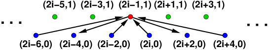
Figure 1. The commutations between $T_{2i-1,1}$ and the other variables of the fundamental cluster ${\mathbf{x}}_{0}$. Vertices $a$ and $b=(2i-1,1)$ are connected by an arrow $a\to b$ iff $T_{a}T_{b}=qT_{b}T_{a}$ and $b\to a$ iff $T_{a}T_{b}=q^{-1}T_{b}T_{a}$, while $T_{a}T_{b}=T_{b}T_{a}$ otherwise.

However, the $A_{1}$ $T$-system comes from an infinite rank cluster algebra with ${\mathbf{x}}_{0}=(x_{i})_{i\in{\mathbb{Z}}}$. We adapt the above condition, based on the quantization of the $A_{1}$ $Q$-system [10, 2], which is a specialization of the $T$-system.

Lemma 3.1.

Let $\Lambda$ be an infinite, skew-symmetric matrix such that

$$(B_{0}\Lambda)_{i,j}=(-1)^{i}(\Lambda_{i+1,j}+\Lambda_{i-1,j})=2\delta_{i,j},\quad i,j\in{\mathbb{Z}},$$

and such that $\Lambda_{i+m,i}=\Lambda_{i-m,i},\ (m>0)$. Then

(3.1) $$\Lambda_{i,j}={1-(-1)^{i+j}\over 2}\times\left\{\begin{matrix}(-1)^{i+j-1\over 2}&{\rm if}\ i\geq j\\ (-1)^{i+j+1\over 2}&{\rm if}\ i<j\end{matrix}\right.$$

The second condition on $\Lambda$ is a choice, a reflection symmetry imposed on the matrix $\Lambda$ which determines the matrix entries (3.1) completely.

The matrix $\Lambda$ encodes the commutation relations among the elements of the fundamental cluster variable ${\mathbf{x}}_{0}$

$$T_{2i-2k,0}T_{2i+1,1} = q^{(-1)^{k}}\,T_{2i+1,1}T_{2i-2k,0},$$

(3.2) $$T_{2i+2k,0}T_{2i-1,1} = q^{(-1)^{k}}\,T_{2i-1,1}T_{2i+2k,0},\quad i\in{\mathbb{Z}},k\geq 0,$$

These commutation relations are depicted graphically in Figure 1.

3.2. The quantum $A_{1}$ $T$-system

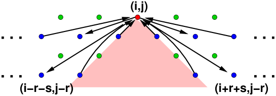
Figure 2. The q-commutations between $T_{i,j}$ and $T_{i+r+s,j-r}$ or $T_{i-r-s,j-r}$ for $r,s\geq 0$ are illustrated as follows: vertices $a$ and $b$ are connected by an arrow $a\to b$ iff $T_{a}T_{b}=qT_{b}T_{a}$. Note that only vertices $a,b$ with heights $j$ of opposite parity give rise to non-trivial commutations. The interior of the shaded cone below $(i,j)$ corresponds to the values $(k,\ell)$ such that $T_{k,\ell}$ cannot belong to the same cluster as $T_{i,j}$.

We define the quantum $A_{1}$ $T$-system for the variables $T_{i,j}$ subject to the commutation relations (3.1) to be:

(3.3) $$q\,T_{i,j+1}T_{i,j-1}=T_{i+1,j}T_{i-1,j}+1\qquad(i,j\in{\mathbb{Z}})$$

As in the commuting system (2.5), this is a “three-term” recursion relation in the variable $j$: All the variables $\{T_{i,j}|i,j\in{\mathbb{Z}},\ i\equiv j\!\!\mod 2\}$ are determined via these equations in terms of the initial data ${\mathbf{x}}_{\mathbf{j}}=(T_{a,j_{a}})_{a\in{\mathbb{Z}}}$ with $|j_{a}-j_{a-1}|=1$.

Mutations $\mu_{a}^{\pm}$ are now implemented by using the relations (3.3) in the forward direction $T_{a,j_{a}}\to T_{a,j_{a}+2}$ or backward direction $T_{a,j_{a}}\to T_{a,j_{a}-2}$.

Using Equations (3.1) and (3.3), the commutation relations between cluster variables within the same seed ${\mathbf{x}}_{{\mathbf{j}}}$ are determined for any ${\mathbf{j}}$.

Lemma 3.2.

Within each admissible initial data set of the quantum $A_{1}$ $T$-system, we have the commutation relations (see Fig.2):

$$T_{i-2k-m,j-m}T_{i,j} = q^{(-1)^{k}{1-(-1)^{m}\over 2}}\,T_{i,j}T_{i-2k-m,j-m}$$

(3.4) $$T_{i+2k+m,j-m}T_{i,j} = q^{(-1)^{k}{1-(-1)^{m}\over 2}}\,T_{i,j}T_{i+2k+m,j-m}$$

for all $i,j\in{\mathbb{Z}}$ and $k,m\in{\mathbb{Z}}_{+}$, with $i+j=0$ mod 2.

Proof.

By induction under mutation. The relations (3.4) reduce to (3.1) for ${\mathbf{x}}_{0}$ under the specialization $j=m=1$.

Suppose the variables in the admissible data set ${\mathbf{x}}_{\mathbf{m}}$ satisfy (3.4) and that $m_{a-1}=m_{a+1}=m_{a}+1=m$ for some fixed value of $a\in{\mathbb{Z}}$. Let us apply (3.3) to perform a mutation $\mu_{a}^{+}:{\mathbf{m}}\to{\mathbf{m}}^{\prime}$ with $m^{\prime}_{b}=m_{b}+2\delta_{b,a}$. We must check that all the commutation relations (3.4) between any $(T_{b,m_{b}})$ for $b\neq a$ and $T_{a,m_{a}^{\prime}}$ hold. Writing $i=a$, $j=m_{a}+1$, the new cluster variable is $T_{i,j+1}$, given by $qT_{i,j+1}T_{i,j-1}=T_{i+1,j}T_{i-1,j}+1$. Let $k=b$, $\ell=m_{b}$ for some $b\neq a$. Without loss of generality, let’s assume that $k=i+r+s$ and $\ell=j-r$, $r\geq 0,s\geq 1$. Then by the commutation relations (3.4), we have

$$T_{i+r+s,j-r}(T_{i+1,j}T_{i-1,j})=(T_{i+1,j}T_{i-1,j})T_{i+r+s,j-r}$$

Henceforth, $T_{i+r+s,j-r}$ must commute with $T_{i,j+1}T_{i,j-1}$, and we obtain

$$T_{i+r+s,j-r}T_{i,j+1}=T_{i,j+1}T_{i+r,j-r-s}q^{-(-1)^{s}{1-(-1)^{r-1}\over 2}}$$

in agreement with (3.4). The Lemma follows. ∎

Remark 3.3.

Note that $T_{i,j}$ and $T_{i^{\prime},j^{\prime}}$ in the same cluster ${\mathbf{x}}_{\mathbf{j}}$ commute if $j\equiv j^{\prime}\mod 2$. From the definition of admissible data sets, we see that $T_{i,j}$and $T_{i^{\prime},j^{\prime}}$ do not belong to the same cluster if $|i-i^{\prime}|<|j-j^{\prime}|$.

Remark 3.4.

Equation (3.3) satisfies a “bar invariance” property in the following sense. Let $*$ denote an algebra antiautomorphism of $\mathcal{A}$, where $q^{*}=q^{-1}$ and $T_{i,i\!\!\mod 2}^{*}=qT_{i,i\!\!\mod 2}$ for $i\in{\mathbb{Z}}$. Then $T_{i,j}^{*}=qT_{i,j}$ for all $i,j\in{\mathbb{Z}}$, $i+j=0$ mod 2. This result is obtained by conjugating the quantum $T$-system (3.3) by $T_{i,j-1}$ and using the commutation relations (3.4).

Using these commutation relations, we see that the $T$-system relation (3.3) is exactly of the form of the quantum cluster mutation (2.4), upon the renormalization of variables $X_{i,j}=q^{1/2}T_{i,j}$. We note that the subset of mutations (3.3) which we consider in the infinite rank cluster algebra makes sense, because the product on the right hand side of a mutation has only a finite number of factors (at most three).

A finite-rank quantum cluster algebra has a Laurent property [2], that is, cluster variables are Laurent polynomials as functions of any cluster seed, as in the case of a commutative cluster algebra. In the quantum case, the coefficients are in ${\mathbb{Z}}[q,q^{-1}]$. It is not completely obvious that this carries over to the current case, which has infinite rank. However we will show that the solutions of the quantum $A_{1}$ $T$-system have the Laurent property, by constructing explicit formulas for the solutions $T_{i,j}$ of the $A_{1}$ quantum $T$-system in terms of any initial data $x_{\mathbf{j}}$. The coefficients are in ${\mathbb{Z}}_{+}[q,q^{-1}]$, which is the analog of the positivity property of cluster algebras [13].

4. Quantum networks and the general solution

Here, we generalize the results of [5] for the network solution of the $T$-system in terms of arbitrary admissible initial data to the non-commutative case. The solution of (3.3) in terms of any given admissible data ${\mathbf{x}}_{j}$ is expressed as a quantum network partition function.

4.1. $U$ and $V$ matrices

Let $a,b$ be elements of $\mathcal{A}$. Define the matrices

(4.1) $$U(a,b)=\begin{pmatrix}1&0\\ q^{-1}b^{-1}&ab^{-1}\end{pmatrix},\qquad V(a,b)=\begin{pmatrix}ab^{-1}&b^{-1}\\ 0&1\end{pmatrix}.$$

These are interpreted as an elementary transfer matrix or “chip”, along a lattice with two rows, going from left to right: $U_{i,j}(a,b)$ or $V_{i,j}(a,b)$ is the weight of the edge connecting the dot (entry connector) in row $i$ on the left to the dot (exit connector) in row $j$ on the right in those elementary chips:

(4.2) $$\qquad\qquad\ U(a,b)\qquad\qquad\qquad\qquad V(a,b)$$

Note that we have represented the variables $a,b$ as attached to the faces of the chips, separated by their edges.

A quantum network is obtained by the concatenation of such chips, forming a chain where the exit connectors $1,2$ of each chip in the chain are identified with the entry connectors of the next chip in the chain, while face labels are well-defined. The latter condition imposes that $U$ and $V$ arguments themselves form a chain $a_{1},a_{2},...$, for instance:

(4.3) $$W=V(a_{1},a_{2})V(a_{2},a_{3})U(a_{3},a_{4})V(a_{4},a_{5})U(a_{5},a_{6})$$

corresponds to the network:

The partition function of a quantum network with matrix of weights $W$ with entry connector $i$ and exit connector $j$ is $W_{i,j}$. It the sum over paths from entry $i$ to exit $j$ of the product on the edges, taken in the order they are traversed.

Lemma 4.1.

Let $a,b,c\in\mathcal{A}$ be invertible elements with relations $ba=qab$ , $bc=qcb$ and $ac=ca$ in $\mathcal{A}$, then

(4.4) $$V(a,b)U(b,c) = U(a,b^{\prime})V(b^{\prime},c),$$

where $b^{\prime}$ is defined by the relation $q\,b^{\prime}b=ac+1$. This definition implies that $cx=qb^{\prime}c$ and $ax=qb^{\prime}a$.

Proof.

Direct calculation:

$$V(a,b)U(b,c)=\begin{pmatrix}(a+c^{-1})b^{-1}&c^{-1}\\ q^{-1}c^{-1}&bc^{-1}\end{pmatrix}$$

and

$$U(a,b^{\prime})V(b^{\prime},c)=\begin{pmatrix}{b^{\prime}}c^{-1}&c^{-1}\\ q^{-1}c^{-1}&q^{-1}{b^{\prime}}^{-1}c^{-1}+a{b^{\prime}}^{-1}\end{pmatrix}$$

Setting the two expressions equal, we find $q{b^{\prime}}b=1+ac$ from the $(1,1)$ element, $q{b^{\prime}}b=1+q{b^{\prime}}a{b^{\prime}}^{-1}c$ from the $(2,2)$ one. Since $a$ commutes with $c$, it commutes with $1+ac$, and the first identity implies that $a{b^{\prime}}b={b^{\prime}}ba=q{b^{\prime}}ab$, i.e. $a{b^{\prime}}=q{b^{\prime}}a$, and $c{b^{\prime}}=q{b^{\prime}}c$. The Lemma follows. ∎

Let ${\mathbf{x}}_{{\mathbf{j}}}$ be admissible data. Then $j_{i}=j_{i+1}\pm 1$. We associate $V^{(i)}({\mathbf{x}}_{\mathbf{j}})=V(T_{i,j_{i}},T_{i+1,j_{i+1}})$ if $j_{i+1}-j_{i}=-1$ and $U^{(i)}({\mathbf{x}}_{\mathbf{j}})=U(T_{i,j_{i}},T_{i+1,j_{i+1}})$ if $j_{i+1}-j_{i}=1$. Thus for the boundary path $(i,j_{i})_{i\in{\mathbb{Z}}}$ on the lattice, $V$ is associated with a down step and $U$ is associated with an up step.

Therefore Lemma 4.1 has a graphical representation in terms of a local mutation of admissible data,

$$\raise-14.22636pt\hbox{${\epsfbox{downup.eps}}$}=\raise-14.22636pt\hbox{${\epsfbox{updown.eps}}$}\\$$

In other words, Lemma 4.1 is an implementation of a mutation of an admissible boundary, using the $A_{1}$ $T$-system. That is, we have the relation

(4.5) $$V^{(i-1)}({\mathbf{x}}_{{\mathbf{j}}})U^{(i)}({\mathbf{x}}_{\mathbf{j}})=U^{(i-1)}({\mathbf{x}}_{{\mathbf{j}}^{\prime}})V^{(i)}({\mathbf{x}}_{{\mathbf{j}}^{\prime}})$$

where ${\mathbf{x}}_{{\mathbf{j}}^{\prime}}=\mu_{i}^{+}({\mathbf{x}}_{\mathbf{j}})$.

4.2. Main Theorem

Let $(i,j)\in{\mathbb{Z}}^{2}$ ($i+j=0\mod 2$) above a fixed admissible boundary ${\mathbf{j}}$, that is, with $j\geq j_{i}$.

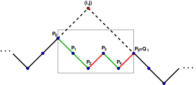
Figure 3. The projection of a point $(i,j)$ onto a given boundary $s_{\mathbf{m}}$.

Definition 4.2.

The projection of the point $(i,j)$ onto the boundary ${\mathbf{j}}$ is the set of points $(i_{0},j_{i_{0}}),(i_{0}+1,j_{i_{0}+1}),\ldots,(i_{1},j_{i_{1}})$, the portion of boundary between the lines $(i+k,j+k)_{k\in{\mathbb{Z}}}$ and $(i+k,j-k)_{k\in{\mathbb{Z}}}$, with endpoints $P_{0}=(i_{0},j_{i_{0}})$ and $Q_{1}=(i_{1},j_{i_{1}})$ such that $j_{i_{0}}-i_{0}=j-i$ with $i_{0}$ maximal and $j_{i_{1}}+i_{1}=j+i$ with $i_{1}$ minimal.

Figure 3 is an example of such a projection. It is a path along the boundary points $(i,j_{i})$ from the vertex $P_{0}$ to the vertex $Q_{1}$ formed by a succession of down (SE) steps $d=(1,-1)$ and up (NE) steps $u=(1,1)$. By definition such a path, if non-empty, starts with a down step and ends up with an up step.

To any path $p=(P_{0},P_{1},P_{2},...,P_{n}=Q_{1})$ made of steps $S_{k}=P_{k}-P_{k-1}\in\{d,u\}$, $k=1,2,...,n$, we associate a matrix product as follows. We define $M_{k}(d,p)=V(T_{P_{k-1}},T_{P_{k}})=V^{(i_{k-1})}({\mathbf{x}}_{\mathbf{j}})$ and $M_{k}(u,p)=U(T_{P_{k-1}},T_{P_{k}})=U^{(i_{k-1})}({\mathbf{x}}_{\mathbf{j}})$, with the matrices $V$ and $U$ as in (4.1) and where for any point of the form $P=(x,y)$ we denote by $T_{P}:=T_{x,y}$. Define

(4.6) $$M(p)=M_{1}(S_{1},p)M_{2}(S_{2},p)\cdots M_{n}(S_{n},p).$$

This product is the weight matrix of the network made up of a concatenation of the basic network chips of the form (4.1) determined by $p$. Let $N(p)$ be the corresponding quantum network.

Example 4.3.

The quantum network $N(p)$ in Equation (4.3) with weight matrix $M(p)=W$ corresponds to the path

$$p=\quad\raise-28.45274pt\hbox{${\epsfbox{pathwork.eps}}$}$$

made of a succession of steps $ddudu$, and with a set of vertices of the form $P_{i-1}=(x_{i},y_{i})\in{\mathbb{Z}}^{2}$ with $x_{i}+y_{i}=0$ mod 2, $i=1,2,...,6$, with $a_{i}=T_{x_{i},y_{i}}$.

The main theorem of this section is the following:

Theorem 4.4.

Let $p$ be the projection of $(i,j)$ onto the boundary ${\mathbf{j}}$, with endpoints $(i_{0},j_{0})\equiv(i_{0},j_{i_{0}})$ and $(i_{1},j_{1})\equiv(i_{1},j_{i_{1}})$. As a function of the admissible data set ${\mathbf{x}}_{{\mathbf{j}}}$,

(4.7) $$T_{i,j}=M(p)_{1,1}T_{i_{1},j_{1}}$$

Proof.

This is proved by induction under mutations of initial data. Let ${\mathbf{x}}_{\mathbf{j}}$ be some initial data whose boundary contains the point $(i,j)$. For such a case, we have $(i,j)=(i_{0},j_{0})=(i_{1},j_{1})$, $T_{i,j}=1\times T_{i,j}=({\mathbf{I}})_{1,1}T_{i_{1},j_{1}}$, and (4.7) is trivially satisfied.

Assume (4.7) holds for some boundary ${\mathbf{x}}_{\mathbf{j}}$, let us show it also holds for the boundary ${\mathbf{x}}_{{\mathbf{j}}^{\prime}}$ with ${\mathbf{j}}^{\prime}=\mu_{a}^{\pm}({\mathbf{j}})$, that is, $j_{a}$ is changed for one value of $a\in{\mathbb{Z}}$, and all other values of $j_{i}$ remain unchanged.

If $a>i_{1}$ or $a<i_{0}$, then the mutation does not affect the formula (4.7), as the boundary ${\mathbf{j}}^{\prime}$ is modified outside of the projection of $(i,j)$ onto it, whereas $M(p)$ and hence $T_{i,j}$ only depends on the boundary values within the projection.

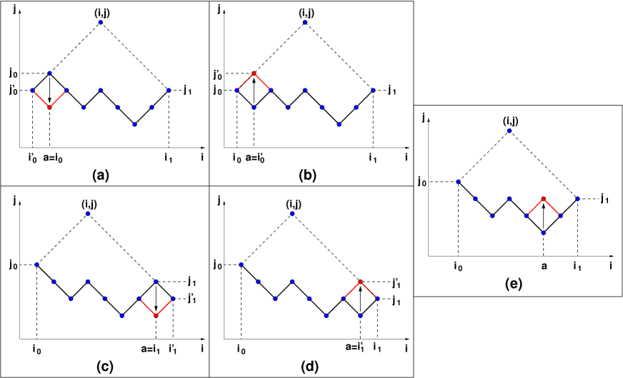
Figure 4. The five cases to be considered in the proof of Theorem 4.4: (a) $a=i_{0}$ (b) $a=i_{0}+1$ (c) $a=i_{1}$ (d) $a=i_{1}-1$ (e) $i_{0}+1<a<i_{1}-1$. For each case, we indicate the mutation by an arrow. The projection of $(i,j)$ onto the boundary is modified by the mutation only in the first four cases.

If $i_{0}\leq a\leq i_{1}$, five situations may occur, as sketched in Fig.4 (a-e). Let $p$ the projection of $(i,j)$ onto ${\mathbf{j}}$, and $p^{\prime}$ the projection of $(i,j)$ onto ${\mathbf{j}}^{\prime}$, and $j_{0}^{\prime}\equiv j_{i_{0}^{\prime}}$, $j_{1}^{\prime}\equiv j_{i_{1}^{\prime}}$.

(a):

If $a=i_{0}$ and $\mu=\mu_{a}^{-}$, then $(i_{0}^{\prime},j_{0}^{\prime})=(i_{0}-1,j_{0}-1)$. The first step of $p$ is must be $d$ for this mutation to be one of the $T$-system equations. Separating out the contribution of this first step of $p$, we write $M(p)=V^{(i_{0})}({\mathbf{j}}){\tilde{M}}(p)$. Using the fact that $(U)_{1,j}=\delta_{j,1}$:

$$M(p)_{1,1} = (U^{(i_{0}-1)}({\mathbf{x}}_{\mathbf{j}})M(p))_{1,1}$$

$$= (U^{(i_{0}-1)}({\mathbf{x}}_{\mathbf{j}})V^{(i_{0})}({\mathbf{x}}_{\mathbf{j}}){\tilde{M}}(p))_{1,1}$$

$$= (V^{(i_{0}-1)}({\mathbf{x}}_{{\mathbf{j}}^{\prime}})U^{(i_{0})}({\mathbf{x}}_{{\mathbf{j}}^{\prime}}){\tilde{M}}(p))_{1,1}=M(p^{\prime})_{1,1}$$

where in the last line, we applied Eq. (4.5). Equation (4.7) follows, as $T_{i_{1},j_{1}}=T_{i^{\prime}_{1},j^{\prime}_{1}}$.

(b):

If $a=i_{0}+1$ and the first two steps of $p$ are $d$, $u$, then $\mu=\mu_{a}^{+}$, $(i_{0}^{\prime},j_{0}^{\prime})=(i_{0}+1,j_{0}+1)$. Therefore,

$$M(p)_{1,1} = (V^{(i_{0})}({\mathbf{x}}_{\mathbf{j}})U^{(i_{0}+1)}({\mathbf{x}}_{\mathbf{j}}){\tilde{M}}(p))_{1,1}$$

$$= (U^{(i_{0})}({\mathbf{x}}_{{\mathbf{j}}^{\prime}})V^{(i_{0}+1)}({\mathbf{x}}_{{\mathbf{j}}^{\prime}}){\tilde{M}}(p))_{1,1}=M(p^{\prime})_{1,1}$$

by application of Eq. (4.5). Equation (4.7) follows, as $T_{i_{1},j_{1}}$ is unchanged by the mutation.

(c):

If $a=i_{1}$ and $\mu=\mu_{a}^{-}$, then $(i_{1}^{\prime},j_{1}^{\prime})=(i_{1}+1,j_{1}-1)$. The last step of $p$ is $u$, so $M(p)={\tilde{M}}(p)U^{(i_{1}-1)}({\mathbf{x}}_{\mathbf{j}})$. Since $(V(a,b))_{i,1}=\delta_{i,1}ab^{-1}$,

$$M(p)_{1,1}T_{i_{1},j_{1}} = \big{(}{\tilde{M}}(p)U^{(i_{1}-1)}({\mathbf{x}}_{\mathbf{j}})V^{(i_{1})}({\mathbf{x}}_{{\mathbf{j}}})\big{)}_{1,1}T_{i_{1}+1,j_{1}-1}$$

$$= \big{(}{\tilde{M}}(p)V^{(i_{1}-1)}({\mathbf{x}}_{{\mathbf{j}}^{\prime}})U^{(i_{1})}({\mathbf{x}}_{{\mathbf{j}}^{\prime}})\big{)}_{1,1}T_{i_{1}+1,j_{1}-1}$$

$$= M(p^{\prime})_{1,1}T_{i_{1}^{\prime},j^{\prime}_{1}}.$$

(d):

If $a=i_{1}-1$ and $\mu=\mu_{a}^{+}$, then $(i_{1}^{\prime},j_{1}^{\prime})=(i_{1}-1,j_{1}+1)$ and the last two steps of $p$ are $d$, $u$. Therefore,

$$M(p)_{1,1}T_{i_{1},j_{1}} = ({\tilde{M}}(p)V^{(i_{1}-2)}({\mathbf{x}}_{\mathbf{j}})U^{(i_{1}-1)}({\mathbf{x}}_{{\mathbf{j}}}))_{1,1}T_{i_{1},j_{1}}$$

$$= ({\tilde{M}}(p)U^{(i_{1}-2)}({\mathbf{x}}_{{\mathbf{j}}^{\prime}})V^{(i_{1}-1)}({\mathbf{x}}_{{\mathbf{j}}^{\prime}}))_{1,1}T_{i_{1},j_{1}}$$

$$= ({\tilde{M}}(p)U^{(i_{1}-2)}({\mathbf{x}}_{{\mathbf{j}}^{\prime}}))_{1,1}T_{i_{1}-1,j_{1}+1}=M(p^{\prime})_{1,1}T_{i_{1}^{\prime},j_{1}^{\prime}}$$

again using $(V(a,b))_{i,1}=\delta_{i,1}ab^{-1}$.

(e):

If $i_{0}+1<a<i_{1}-1$, the endpoints of the projection onto the boundary do not change and the mutation $\mu_{a}^{\pm}$ amounts to a change of ordering of one pair of factors within the product $M(p)$ of the form (4.5), which corresponds to writing it as $M(p^{\prime})$, $p^{\prime}=\mu_{a}^{\pm}(p)$ and (4.7) follows.

∎

Theorem 4.4 may be rephrased in the language of a quantum network partition function:

Corollary 4.5.

The quantity $T_{i,j}T_{i_{1},j_{1}}^{-1}$ is the partition function of the quantum network $N(p)$, with weight matrix $M(p)$, with entry and exit connector $1$, where $p$ is the projection of $(i,j)$ onto the boundary.

As all weights involved in the network $N(p)$ are Laurent monomials of the initial data ${\mathbf{x}}_{{\mathbf{j}}}$ with coefficients in ${\mathbb{Z}}_{+}[q,q^{-1}]$, we deduce the following positivity result, the quantum version of the Fomin-Zelevinsky positivity conjecture:

Corollary 4.6.

The expression for $T_{i,j}$ in terms of any initial data $x_{\mathbf{j}}$ is a Laurent polynomial with coefficients in ${\mathbb{Z}}_{+}[q,q^{-1}]$.

Example 4.7.

Consider the case where $(i,j)=(0,4)$, with a boundary projection of the form: $p=((-2,2),(-1,1),(0,0),(1,1),(2,2))$. Then $(i_{0},j_{0})=(-2,2)$, $(i_{1},j_{1})=(2,2)$. It consists of the steps $dduu$, hence

$$M(p)=V^{(-2)}({\mathbf{x}}_{\mathbf{j}})V^{(-1)}({\mathbf{x}}_{\mathbf{j}})U^{(0)}({\mathbf{x}}_{\mathbf{j}})U^{(1)}({\mathbf{x}}_{\mathbf{j}})$$

which yields

$$T_{0,4}=M(p)_{1,1}T_{2,2}=T_{-2,2}T_{0,0}^{-1}T_{2,2}+q^{-1}(T_{-2,2}T_{-1,1}^{-1}T_{0,0}^{-1}+T_{-1,1}^{-1})(T_{1,1}^{-1}T_{2,2}+T_{0,0}T_{1,1}^{-1})$$

The five monomials forming $T_{0,4}T_{2,2}^{-1}$ are the weights of the five paths $1\to 1$ in the network $N(p)$ with weight matrix $M(p)$:

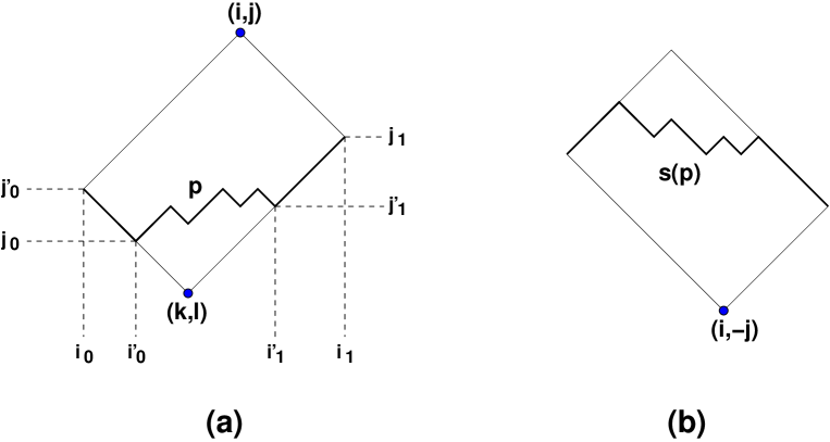
Figure 5. (a) The projection of a point $(i,j)$ onto a boundary ${\mathbf{j}}$, and the corresponding point $(k,l)$. (b) The action of the reflection $s:(i,j)\mapsto(i,-j)$.

Finally, we can use the symmetry of the $T$-system under the bar involution to compute $T_{k,\ell}$ with $\ell\leq j_{k}$. Given a boundary ${\mathbf{j}}$ and a point $(i,j)$ above it with $j\geq j_{i}$, let $p$ denote the projection of $(i,j)$ onto the boundary with endpoints $(i_{0},j_{0})$ and $(i_{1},j_{1})$. Then

$$i={i_{0}+i_{1}+j_{1}-j_{0}\over 2},\qquad j={j_{0}+j_{1}+i_{1}-i_{0}\over 2}.$$

Let $(k,l)$ be the point under the boundary such that

(4.8) $$k={i_{0}+i_{1}+j_{0}-j_{1}\over 2},\qquad l={j_{0}+j_{1}+i_{0}-i_{1}\over 2}.$$

(See Fig.5 (a) for an illustration.). Let $s:(i,j)\mapsto(i,-j)$ denote a reflection. Under $s$, the boundary ${\mathbf{j}}$ is sent to $-{\mathbf{j}}$ (see Fig.5 (b)). The projection of $s(k,l)$ onto the reflected boundary $-{\mathbf{j}}$ is $s(p^{\prime})$, a sub-path of $s(p)$, with endpoints $s(i_{0}^{\prime},j_{0}^{\prime})$ and $s(i_{1}^{\prime},j_{1}^{\prime})$, with $i_{0}-i_{0}^{\prime}=j_{0}-j_{0}^{\prime}\geq 0$ and $i_{1}^{\prime}-i_{1}=j_{1}-j_{1}^{\prime}\geq 0$. Note that $s(p)=u^{i_{0}-i_{0}^{\prime}}s(p^{\prime})d^{i_{1}^{\prime}-i_{1}}$. We have the following:

Theorem 4.8.

Let ${\mathbf{j}}$, $(i,j)$, $p$ and $M(p)$ be as in Theorem 4.4, and $(k,l)$ the point under the boundary ${\mathbf{j}}$ defined by (4.8). In terms of the initial data ${\mathbf{x}}_{\mathbf{j}}$, we have:

(4.9) $$T_{k,l}=\big{(}M(p)\big{)}_{2,2}T_{i_{1},j_{1}}.$$

Proof.

Note first that $S_{i,j}=qT_{i,-j}$ is a solution of the $A_{1}$ quantum $T$-system with $q\to q^{-1}$. Indeed, from (3.3), $q^{-1}S_{i,j-1}S_{i,j+1}=q^{-2}S_{i+1,j}S_{i-1,j}+1$, and upon applying the bar involution of Remark 3.4, $q^{-1}S_{i,j+1}S_{i,j-1}=S_{i+1,j}S_{i-1,j}+1$. Therefore with the initial data $q{\mathbf{x}}_{-{\mathbf{j}}}=(qT_{i,j_{i}})_{i\in{\mathbb{Z}}}$, we have

$$q^{-1}S_{i,j}=T_{i,-j}=M(p,q{\mathbf{x}}_{-{\mathbf{j}}},q^{-1})_{1,1}q^{-1}S_{i_{1},j_{1}}=M(p,q{\mathbf{x}}_{-{\mathbf{j}}},q^{-1})_{1,1}T_{i_{1},-j_{1}}$$

Here, we have made explicit the arguments of $M(p):=M(p,{\mathbf{y}},t)$, where ${\mathbf{y}}$ is the boundary data in the $V,U$ matrices, and the quantum parameter is $t$. Similarly, let $U^{(i)}({\mathbf{y}})=U^{(i)}({\mathbf{y}},t)$ and $V^{(i)}({\mathbf{y}})=V^{(i)}({\mathbf{y}},t)$ where $t$ is the quantum parameter. Then $M(p,q{\mathbf{x}}_{-{\mathbf{j}}},q^{-1})$ is obtained from $M(p,{\mathbf{x}}_{\mathbf{j}},q)$ upon substitution of the matrices

$$U^{(i)}({\mathbf{x}}_{\mathbf{j}},q)\mapsto U^{(i)}(q{\mathbf{x}}_{-{\mathbf{j}}},q^{-1})\quad{\rm and}\quad V^{(i)}({\mathbf{x}}_{\mathbf{j}},q)\mapsto V^{(i)}(q{\mathbf{x}}_{-{\mathbf{j}}},q^{-1})$$

We note that

$$U(qa,qb;q^{-1})=JV(a,b;q)J\quad{\rm and}\quad V(qa,qb;q^{-1})=JU(a,b;q)J$$

where $J=\begin{pmatrix}0&1\\ 1&0\end{pmatrix}$ is the permutation matrix. Therefore,

$$T_{i,-j}=(JM(s(p),{\mathbf{x}}_{-{\mathbf{j}}},q)J)_{1,1}T_{i_{1},-j_{1}}=M(s(p),{\mathbf{x}}_{-{\mathbf{j}}},q)_{2,2}T_{i_{1},-j_{1}}$$

where $s(p)$ is the reflected path with $d$ and $u$ steps interchanged. This last identity corresponds to the reflecting of the entire initial picture. Upon renaming $(i,-j)\to(k,l)$, $(i_{1},-j_{1})\to(i_{1}^{\prime},j_{1}^{\prime})$, $(i_{0},-j_{0})\to(i_{0}^{\prime},j_{0}^{\prime})$, $s(p)\to p^{\prime}$, and ${\mathbf{x}}_{-{\mathbf{j}}}\to{\mathbf{x}}_{\mathbf{j}}$, we deduce that

$$T_{k,l}=M(p^{\prime})_{2,2}T_{i_{1}^{\prime},j_{1}^{\prime}}$$

Recalling finally that $p=d^{i_{0}-i_{0}^{\prime}}p^{\prime}u^{i_{1}^{\prime}-i_{1}}$ and that, due to the particular triangular form of the $U,V$ matrices:

$$\left(\prod_{i=i_{0}^{\prime}}^{i_{0}-1}V^{(i)}({\mathbf{x}}_{\mathbf{j}})\right)_{2,m}=\delta_{m,2},\qquad\left(\prod_{i=i_{1}}^{i_{1}^{\prime}-1}U^{(i)}({\mathbf{x}}_{\mathbf{j}})\right)_{m,2}=\delta_{m,2}T_{i_{1}^{\prime},j_{1}^{\prime}}T_{i_{1},j_{1}}^{-1},$$

the Theorem follows. ∎

4.3. Conserved quantities and $V,U$ matrices

In this section we investigate the content of the full network matrix $M(p)$ of Theorems 4.4 and 4.8, in the special case of the fundamental boundary ${\mathbf{j}}_{0}$, with heights $j_{i}=i\mod 2$.

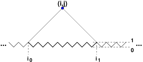
Figure 6. The projection of a point $(i,j)$ onto the fundamental boundary ${\mathbf{j}}_{0}$.

Let $p$ be the projection of $(i,j)\in{\mathbb{Z}}^{2}$ with $j\geq(i\ {\rm mod}\ 2)$ onto the boundary ${\mathbf{j}}_{0}$, consisting of vertices $\{(a,j_{a})\,:\,i_{0}\leq a\leq i_{1}\}$ with $i_{0},i_{1}$ odd (see Fig.6).

We have

$$M(p)=(V^{(i_{0})}U^{(i_{0}+1)}\cdots V^{(i_{1}-2)}U^{(i_{1}-1)})({\mathbf{x}}_{\mathbf{j}}).$$

Let $n=(i_{1}-i_{0})/2$, then the length of $p$ is $2n$.

We focus on the non-diagonal terms of $M(p)T_{i_{1},1}$. These involve what we call (in analogy with the commutative case) the conserved quantities of the quantum $A_{1}$ $T$-system:

Lemma 4.9.

Let $(i,j)\in{\mathbb{Z}}^{2}$, and $T$ a solution of the quantum $A_{1}$ $T$-system (3.3). Then

$$c_{i,j}=T_{i-1,j+1}T_{i,j}^{-1}+T_{i,j}^{-1}T_{i+1,j-1}$$

is independent of $i-j$ and

$$d_{i,j}=T_{i-1,j-1}T_{i,j}^{-1}+T_{i,j}^{-1}T_{i+1,j+1}$$

is independent of $i+j$. That is,

$$c_{i,j}=c_{i-1,j-1}=c_{i-j,0}:=c_{i-j}\qquad d_{i,j}=d_{i+1,j-1}=d_{i+j,0}:=d_{i+j}$$

Proof.

We write the $T$-system equations:

$$\left\{\begin{matrix}qT_{i,j}T_{i,j-2}=T_{i+1,j-1}T_{i-1,j-1}+1\hfill&\Rightarrow T_{i-1,j-1}^{-1}T_{i,j-2}=T_{i,j}^{-1}T_{i+1,j-1}+T_{i,j}^{-1}T_{i-1,j-1}^{-1}\hfill\\ qT_{i-1,j+1}T_{i-1,j-1}=T_{i,j}T_{i-2,j}+1\hfill&\Rightarrow T_{i-1,j+1}T_{i,j}^{-1}=T_{i-2,j}T_{i-1,j-1}^{-1}+T_{i,j}^{-1}T_{i-1,j-1}^{-1}\hfill\end{matrix}\right.$$

where in the first line we have used the $q$-commutation of $T_{i-1,j-1}^{-1}$ and $T_{i,j-2}$ and that of $T_{i-1,j+1}$ and $T_{i,j}^{-1}$ in the second. Subtracting these last two equations leads to $c_{i,j}=c_{i-1,j-1}$. The conservation of $d$ is proved in a similar manner. ∎

We also define by induction the following polynomials of the conserved quantities:

$$\left\{\begin{matrix}\varphi^{(-1)}_{m}=0,&\varphi^{(0)}_{m}=1,&\varphi^{(p)}_{m}=\varphi^{(p-1)}_{m}c_{m+2p-2}-q\,\varphi^{(p-2)}_{m}\hfill\\ \theta^{(-1)}_{m}=0,&\theta^{(0)}_{m}=1,&\theta^{(p)}_{m}=d_{m+2-2p}\,\theta^{(p-1)}_{m}-q^{-1}\theta^{(p-2)}_{m}\hfill\end{matrix}\right.\quad(p\geq 1,m\in{\mathbb{Z}})$$

Note that, while it is true that $[c_{m},d_{p}]=0=[\varphi^{(i)}_{m},\theta^{(j)}_{p}]$, for all $i,j,m,p$, neither the $c$’s nor the $d$’s commute among themselves.

We have:

Theorem 4.10.

Let $(i,j)$ be a point above the boundary ${\mathbf{j}}={\mathbf{j}}_{0}$ and $p$ be the projection of $(i,j)$ onto the boundary, $p$ a zig-zag path with endpoints $(i_{0},1)$ and $(i_{1},1)$ and length $2n=i_{1}-i_{0}$, as in Fig.6. Then

$$\big{(}M(p)\big{)}_{1,2}\,T_{i_{1},1} = \varphi^{(n-1)}_{i-j+2},$$

$$\big{(}M(p)\big{)}_{2,1}\,T_{i_{1},1} = q^{-1}\,\theta^{(n-1)}_{i+j-2}.$$

Proof.

By induction on $n$. For $n=0$, $M(p)={\mathbf{I}}$, and the theorem holds, as $\varphi^{(-1)}_{m}=\theta^{(-1)}_{m}=0$.

Assume the theorem holds for paths $p^{\prime}$ of length $2n$. Let $p$ be a path of length $2n+2$, with $i_{0}=i-n-1$, $i_{1}=i+n+1$, $j=n+2$. Denote by $p^{\prime}$ the truncated projection between the lines $i=i_{0}$ and $i=i_{1}-2$. For simplicity, we introduce the following notation: $U^{(i)}({\mathbf{x}}_{\mathbf{j}})=\langle i|U|i+1\rangle$ and $V^{(i)}({\mathbf{x}}_{\mathbf{j}})=\langle i|V|i+1\rangle$, with $|i\rangle\langle i|=I$ for all $i$. We have

(4.10) $$(M(p))_{1,2}T_{i_{1},1} = \big{(}\langle i_{0}|(VU)^{n+1}|i_{1}\rangle\big{)}_{1,2}T_{i_{1},1}$$

$$= \big{(}\langle i_{0}|(VU)^{n}|i_{1}-2\rangle\langle i_{1}-2|VU|i_{1}\rangle)\big{)}_{1,2}T_{i_{1},1}$$

$$= \big{(}M(p^{\prime})\langle i_{1}-2|V|i_{1}-1\rangle)\big{)}_{1,2}T_{i_{1}-1,0}$$

$$= (M(p^{\prime}))_{1,2}T_{i_{1}-2,1}T_{i_{1}-2,1}^{-1}T_{i_{1}-1,0}+(M(p^{\prime}))_{1,1}$$

$$= \varphi^{(n-1)}_{i-j+2}T_{i_{1}-2,1}^{-1}T_{i_{1}-1,0}+T_{i-1,j-1}T_{i_{1}-2,1}^{-1}$$

by applying Theorem 4.4. Repeating this calculation for $(M(p^{\prime}))_{1,2}T_{i_{1}-2,1}=\varphi^{(n-1)}_{i-j+2}$ by the recursion hypothesis, we get analogously:

$$\varphi^{(n-1)}_{i-j+2}=\varphi^{(n-2)}_{i-j+2}T_{i_{1}-4,1}^{-1}T_{i_{1}-3,0}+T_{i-2,j-2}T_{i_{1}-4,1}^{-1}$$

We may consider this identity with indices $i,j$ shifted by $+1$, while $n$ remains fixed, namely

$$\varphi^{(n-1)}_{i-j+2}=\varphi^{(n-2)}_{i-j+2}T_{i_{1}-3,2}^{-1}T_{i_{1}-2,1}+T_{i-1,j-1}T_{i_{1}-3,2}^{-1}$$

from which we deduce:

$$\varphi^{(n-1)}_{i-j+2}T_{i_{1}-3,2}T_{i_{1}-2,1}^{-1} = \varphi^{(n-2)}_{i-j+2}T_{i_{1}-3,2}^{-1}T_{i_{1}-2,1}T_{i_{1}-3,2}T_{i_{1}-2,1}^{-1}+T_{i-1,j-1}T_{i_{1}-2,1}^{-1}$$

$$= q\,\varphi^{(n-2)}_{i-j+2}+T_{i-1,j-1}T_{i_{1}-2,1}^{-1}$$

by use of the $q$ commutation of $T_{i_{1}-2,1}$ and $T_{i_{1}-3,2}$. Comparing with (4.10), we finally get

$$(M(p))_{1,2}T_{i_{1},1} = \varphi^{(n-1)}_{i-j+2}(T_{i_{1}-3,2}T_{i_{1}-2,1}^{-1}+T_{i_{1}-2,1}^{-1}T_{i_{1}-1,0})-q\,\varphi^{(n-2)}_{i-j+2}$$

$$= \varphi^{(n-1)}_{i-j+2}c_{i+n-2}-q\,\varphi^{(n-2)}_{i-j+2}=\varphi^{(n-1)}_{i-j+2}c_{i-j+2n}-q\,\varphi^{(n-2)}_{i-j+2}=\varphi^{(n)}_{i-j+2}$$

by the defining recursion relation for $\varphi^{(n)}_{m}$. The second statement of the theorem follows analogously. ∎

5. Quantum $Q$-system for $A_{1}$ and its fully non-commutative version

5.1. Quantum $Q$-system: from the path solution to the network solution

5.1.1. $A_{1}$ $Q$-system

Closely related to the $A_{1}$ $T$-system is the $A_{1}$ $Q$-system:

(5.1) $$R_{j+1}R_{j-1}=R_{j}^{2}+1\qquad(j\in{\mathbb{Z}})$$

which is satisfied by the 2-periodic solutions of the $A_{1}$ $T$-system in $i$, namely with $T_{i+2,j}=T_{i,j}=T_{j\,{\rm mod}\,2,j}=R_{j}$. The admissible initial data are of the form ${\mathbf{x}}_{n}=(R_{n},R_{n+1})$ and are the restrictions of the $2$-periodic initial data of the $T$-system with ${\mathbf{j}}$ such that $j_{i}=n$ if $i-n=0$ mod 2, and $j_{i}=n+1$ otherwise.

The $A_{1}$ $Q$-system (5.1) has an associated cluster algebra [17] with fundamental seed made of the cluster ${\mathbf{x}}_{0}=(R_{0},R_{1})$ and of the exchange matrix $B_{0}=\begin{pmatrix}0&2\\ -2&0\end{pmatrix}$. A forward mutation $\mu^{+}:{\mathbf{x}}_{n}\mapsto{\mathbf{x}}_{n+1}$ takes $R_{n}\to R_{n+2}=(R_{n+1}^{2}+1)/R_{n}$, while a backward one $\mu^{-}:{\mathbf{x}}_{n}\mapsto{\mathbf{x}}_{n-1}$ takes $R_{n+1}\to R_{n-1}=(R_{n}^{2}+1)/R_{n+1}$.

5.1.2. Quantum $A_{1}$ $Q$-system from quantum cluster algebra

The quantum cluster algebra associated to the cluster algebra of the $A_{1}$ $Q$-system (5.1), is obtained by taking the admissible pair $(B_{0},\Lambda)$ with $\Lambda=2(B_{0})^{-1}=\begin{pmatrix}0&1\\ -1&0\end{pmatrix}$ (see Ref.[2, 10]), which amounts to the commutation relation $R_{0}R_{1}=q\,R_{1}R_{0}$ for the fundamental initial data ${\mathbf{x}}_{0}=(R_{0},R_{1})$. The quantum $A_{1}$ $Q$-system [2, 10] expresses the mutations of the quantum cluster algebra, and reads:

(5.2) $$qR_{j+1}R_{j-1}=R_{j}^{2}+1\qquad(j\in{\mathbb{Z}})$$

Together with the above fundamental initial data, compatibility implies the following commutation relation holds within each cluster ${\mathbf{x}}_{n}=(R_{n},R_{n+1})$:

(5.3) $$R_{n}R_{n+1}=q\,R_{n+1}R_{n}$$

Note that, like in the commuting case, the solutions of the quantum $A_{1}$ $Q$-system (5.2) are the solutions of the quantum $A_{1}$ $T$-system (3.3) that are $2$-periodic in the index $i$, namely with $R_{j}=T_{j\!\!\mod 2,j}$.

5.1.3. Solution via quantum paths v/s quantum networks

The quantum $A_{1}$ $Q$-system (5.2) was solved in [10] in terms of “quantum” paths as follows. Let us define weights

(5.4) $$y_{1}=R_{1}R_{0}^{-1}\qquad y_{2}=R_{1}^{-1}R_{0}^{-1}\qquad y_{3}=R_{1}^{-1}R_{0}$$

These weights satisfy the relations:

$$y_{1}y_{3}=y_{3}y_{1}=q\qquad y_{1}y_{2}=q^{2}\,y_{2}y_{1}\qquad y_{2}y_{3}=q^{2}\,y_{3}y_{2}$$

We consider “quantum” paths on the integer segment $[0,3]$ from and to the origin $0$, with steps $\pm 1$ with weight $1$ for $i\to i+1$, $i=0,1,2$ and $y_{i}$ for $i\to i-1$, $i=1,2,3$. The weight of a path $p$, $w(p)$ is the product of the step weights in the order in which they are taken. The partition function for quantum paths of length $2j$ is the sum over the paths $p$ from and to the origin, with $2j$ steps, of the weights $w(p)$. We have the following

Theorem 5.1.

([10]) For $j\in{\mathbb{Z}}_{+}$, the solution $R_{j}$ to the quantum $A_{1}$ $Q$-system (5.2) is equal to the partition function for quantum paths of length $2j$, times $R_{0}$.

A reformulation of this result uses the “two-step” transfer matrix $\mathcal{T}$ whose entries are the weights of the paths of length $2$ that start (and end) at the even points $0$ and $2$:

(5.5) $$\mathcal{T}=\begin{pmatrix}y_{1}&1\\ y_{2}y_{1}&y_{2}+y_{3}\end{pmatrix}=\begin{pmatrix}w\left(\raise-5.69046pt\hbox{${\epsfbox{t11.eps}}$}\right)&w\left(\raise-11.38092pt\hbox{${\epsfbox{t12.eps}}$}\right)\\ w\left(\raise-11.38092pt\hbox{${\epsfbox{t21.eps}}$}\right)&w\left(\raise-5.69046pt\hbox{${\epsfbox{t22.eps}}$}\right)\end{pmatrix}$$

The theorem may be rephrased as the following identity:

(5.6) $$R_{j}=(\mathcal{T}^{j})_{1,1}\,R_{0}\qquad(j\in{\mathbb{Z}}_{+})$$

We may now apply the Theorem 4.4 above to obtain an alternative quantum network formulation of the $A_{1}$ $Q$-system solutions. We start with the fundamental initial data $x_{0}=(R_{0},R_{1})$, with $R_{0}R_{1}=qR_{1}R_{0}$. We have by Theorem 4.4, for all $j\in{\mathbb{Z}}_{>0}$:

(5.7) $$R_{j}=T_{j\,{\rm mod}\,2,j}=\big{(}(VU)^{j-1}\big{)}_{1,1}R_{1}=\big{(}(UV)^{j}\big{)}_{1,1}R_{0}$$

where, due to the periodicity property, we have

$$V=V(R_{1},R_{0})=\begin{pmatrix}R_{1}R_{0}^{-1}&R_{0}^{-1}\\ 0&1\end{pmatrix}\qquad U=U(R_{0},R_{1})=\begin{pmatrix}1&0\\ q^{-1}R_{1}^{-1}&R_{0}R_{1}^{-1}\end{pmatrix}$$

$$UV=\begin{pmatrix}R_{1}R_{0}^{-1}&R_{0}^{-1}\\ q^{-1}R_{0}^{-1}&(R_{0}+R_{0}^{-1})R_{1}^{-1}\end{pmatrix}=\begin{pmatrix}y_{1}&R_{0}^{-1}\\ q^{-1}R_{0}^{-1}&q^{-1}(y_{2}+y_{3})\end{pmatrix}$$

Comparing with eq.(5.5), and noting that $y_{2}y_{1}=R_{1}^{-1}R_{0}^{-1}R_{1}R_{0}^{-1}=q^{-1}R_{0}^{-2}$, and that $R_{0}^{-1}(y_{2}+y_{3})R_{0}=q^{-1}(y_{2}+y_{3})$, we arrive at the relation:

(5.8) $$UV=\begin{pmatrix}1&0\\ 0&R_{0}^{-1}\end{pmatrix}\mathcal{T}\begin{pmatrix}1&0\\ 0&R_{0}\end{pmatrix}$$

from which we deduce that Eqns. (5.6) and (5.7) are equivalent, as the conjugation does not affect the $(1,1)$ matrix element.

5.2. Non-commutative $Q$-system: a solution via non-commutative networks

The fully non-commutative version of the $A_{1}$ $Q$-system was studied and solved in [9]. It reads:

(5.9) $$R_{n+1}R_{n}^{-1}R_{n-1}=R_{n}+R_{n}^{-1}\qquad(n\in{\mathbb{Z}})$$

for $R_{n}$ some formal non-commutative variables subject to the quasi-commutation relations

(5.10) $$R_{n}R_{n+1}=R_{n+1}CR_{n}$$

where $C$ is another fixed non-commuting variable. The quantum case is recovered when $C=q$ is central.

Using the relations (5.10), the non-commutative $A_{1}$ $Q$-system (5.9) may be rewritten as

(5.11) $$R_{n+1}CR_{n-1}=R_{n}^{2}+1\qquad(n\in{\mathbb{Z}})$$

Let us keep the definition (5.4) for $y_{1},y_{2},y_{3}$, now in terms of the non-commutative initial data $R_{0}$ and $R_{1}$. The solution of [9] involves “non-commutative paths” from and to the origin on $[0,3]$, with weights $1$ for the steps $i\to i+1$, $i=0,1,2$ and $y_{i}$ for the steps $i\to i-1$, $i=1,2,3$. We have:

Theorem 5.2.

([9]) For $n\in{\mathbb{Z}}_{+}$, the solution $R_{n}$ of the non-commutative $A_{1}$ $Q$-system is the partition function for non-commutative paths from the origin to itself with $2n$ steps, times $R_{0}$.

As before, this is best expressed by use of the “two-step” transfer matrix $\mathcal{T}$, still given by the expression (5.5) in terms of $R_{0}$ and $R_{1}$, and the identity (5.6) still holds.

The network solution of the quantum $A_{1}$ $Q$-system may be adapted for the fully non-commutative one as follows. For non-commuting variables $a,b$, we introduce the matrices:

(5.12) $$U(a,b)=\begin{pmatrix}1&0\\ C^{-1}b^{-1}&ab^{-1}\end{pmatrix}\qquad V(a,b)=\begin{pmatrix}ab^{-1}&b^{-1}\\ 0&1\end{pmatrix}$$

We have the following generalization of Lemma 4.1.

Lemma 5.3.

Assume $a,b,c$ have the quasi-commutations $ba=aCb$, $bc=cCb$, and $ac=ca$, then we have the equation:

(5.13) $$V(a,b)U(b,c)=U(a,b^{\prime})V(b^{\prime},c)$$

for $b^{\prime}$ defined via $b^{\prime}Cb=ac+1$. Moreover, with this definition, $cb^{\prime}=b^{\prime}Cc$ and $ab^{\prime}=b^{\prime}Ca$.

Proof.

We compute directly

$$V(a,b)U(b,c)=\begin{pmatrix}ab^{-1}&b^{-1}\\ 0&1\end{pmatrix}\begin{pmatrix}1&0\\ C^{-1}c^{-1}&bc^{-1}\end{pmatrix}=\begin{pmatrix}(a+c^{-1})b^{-1}&c^{-1}\\ C^{-1}c^{-1}&bc^{-1}\end{pmatrix}$$

and

$$U(a,b^{\prime})V(b^{\prime},c)=\begin{pmatrix}1&0\\ C^{-1}b^{\prime-1}&ab^{\prime-1}\end{pmatrix}\begin{pmatrix}b^{\prime}c^{-1}&c^{-1}\\ 0&1\end{pmatrix}=\begin{pmatrix}b^{\prime}c^{-1}&c^{-1}\\ C^{-1}c^{-1}&C^{-1}b^{\prime-1}c^{-1}+ab^{\prime-1}\end{pmatrix}$$

Identifying the two results, we obtain $b^{\prime}c^{-1}bc=b^{\prime}Cb=1+ac$ from the (1,1) element identification, and $b^{\prime}Cb=1+b^{\prime}Cab^{\prime-1}c$ from the $(2,2)$ one. But from the first identity we deduce that $ab^{\prime}=b^{\prime}Ca$ (as well as $cb^{\prime}=b^{\prime}Cc$), and the Lemma follows. ∎

Theorem 5.4.

For $n\in{\mathbb{Z}}_{+}$, $p\in{\mathbb{Z}}$, the solution $R_{n+p}$ of the non-commutative $A_{1}$ $Q$-system is expressed in terms of the initial data $x_{p}=(R_{p},R_{p+1})$ as:

$$R_{n+p}=\big{(}(V_{p}U_{p})^{n-1}\big{)}_{1,1}R_{p+1}=\big{(}(U_{p}V_{p})^{n}\big{)}_{1,1}R_{p}$$

where $V_{p}=V(R_{p+1},R_{p})$ and $U_{p}=U(R_{p},R_{p+1})$ in terms of the matrices of eq.(5.12).

Proof.

By induction on $n$. The result is clear for $n=1$. Assume that the Theorem holds for $n-1,p+1$. Applying the Lemma 5.3 for $a=c=R_{p+1}$ and $b=R_{p}$, we get $x=R_{p+2}$ and $V_{p}U_{p}=U_{p+1}V_{p+1}$. We deduce that:

$$\big{(}(V_{p}U_{p})^{n-1}\big{)}_{1,1}R_{p+1}=\big{(}(U_{p+1}V_{p+1})^{n-1}\big{)}_{1,1}R_{p+1}=R_{(n-1)+(p+1)}=R_{n+p}$$

and the Theorem holds for $n,p$. Finally, the translational invariance of (5.11) implies that $R_{n+p}$ is the same function of $(R_{p},R_{p+1})$ as $R_{n}$ of $(R_{0},R_{1})$, independently of $p\in{\mathbb{Z}}$. The Theorem follows. ∎

The direct connection between the non-commutative network formulation and the non-commutative path formulation is the same relation (5.8) between $VU$ and $\mathcal{T}$ as in the quantum case. It is now a consequence of: $y_{2}y_{1}=R_{1}^{-1}R_{0}^{-1}R_{1}R_{0}^{-1}=R_{0}^{-1}C^{-1}R_{0}^{-1}$ and $R_{0}(y_{2}+y_{3})R_{0}^{-1}=C^{-1}R_{1}^{-1}R_{0}^{-1}+R_{0}R_{1}^{-1}$, by use of the quasi-commutations (5.10).

6. Discussion: connection to the quantum lattice Liouville equation

In this paper, we have introduced and solved the quantum $A_{1}$ $T$-system in terms of an arbitrary admissible data, by means of a quantum path model. This system turns out to be closely related to the quantum lattice Liouville equation of [12].

The $T$-systems in general are related to the so-called $Y$-systems via a birational transformation [21]. The following is a quantum version of this transformation. Define

$$\chi_{i,j}=\left(T_{i+1,j}T_{i-1,j}\right)^{-1}\qquad(i,j\in{\mathbb{Z}}).$$

Then

$$\chi_{i,j-1}\chi_{i,j+1} = T_{i+1,j-1}^{-1}(T_{i-1,j+1}T_{i-1,j-1})^{-1}T_{i+1,j+1}^{-1}$$

$$= qT_{i+1,j-1}^{-1}(1+T_{i,j}T_{i-2,j})^{-1}T_{i+1,j+1}^{-1}$$

$$= q(T_{i+1,j+1}T_{i+1,j-1})^{-1}(1+T_{i,j}T_{i-2,j})^{-1}$$

$$= q^{2}\chi_{i+1,j}(1+\chi_{i+1,j})^{-1}\chi_{i-1,j}(1+\chi_{i-1,j})^{-1}.$$

Note that all the factors in the last line commute.

This system may be called quantum $Y$-system for $A_{1}$: If we set $q=1$ and denote $Y_{i}(j/2)=\chi_{i,j}$ it coincides with the $A_{1}$ $Y$-system [25, 24]. In the non-commuting case, it coincides (upon a reordering of the left hand side and a renormalization of the variables, $\chi\mapsto q\chi$) with the quantum lattice Liouville equations of [12].

The variables $\chi_{i,j}$ have local commutation relations within each cluster.

Lemma 6.1.

$$\chi_{k\pm 1,l+1}\chi_{k,l}=q^{2}\chi_{k,l}\chi_{k\pm 1,l+1},$$

while all other pairs of variables commute.

Proof.

Let $j\geq l$. If $(i,j)\neq(k,l+1)$, then the commutation relations (3.4) imply that $T_{i,j}\chi_{k,l}=\chi_{k,l}T_{i,j}.$ Otherwise,

$$T_{k,l+1}\chi_{k,l}=T_{k,l+1}T_{k+1,l}^{-1}T_{k-1,l}^{-1}=q^{2}\chi_{k,l}T_{k,l+1},$$

and the Lemma follows. ∎

Note that here we do not impose the periodicity condition of [12], that $\chi_{i+2N,j}=\chi_{i,j}$. Here it would be implemented by a periodicity condition of the form $T_{i+2N,j}=T_{i,j}$. The solution of this paper holds for any choice of boundary conditions, and may therefore be restricted to these special periodicity conditions on $T_{i,j}$.

References

- [1] I. Assem, C. Reutenauer, and D. Smith Frises, arXiv:0906.2026 [math.RA].
- [2] A. Berenstein, A. Zelevinsky, Quantum Cluster Algebras, Adv. Math. 195 (2005) 405–455. arXiv:math/0404446 [math.QA].
- [3] P. Caldero and M. Reineke, On the quiver Grassmannian in the acyclic case. J. Pure Appl. Algebra 212 (2008), no. 11, 2369–2380. arXiv:math/0611074 [math.RT].
- [4] H.S.M. Coxeter, Frieze Patterns, Triangulated Polygons and Dichromatic Symmetry, in The Lighter Side of Mathematics, R.K. Guy and E. Woodrow (eds.), John Wiley Sons, NY, (1961) pp 15-27.
- [5] P. Di Francesco, The solution of the T-system for arbitrary boundary, Elec. Jour. of Comb. Vol. 17(1) (2010) R89. arXiv:1002.4427 [math.CO].
- [6] P. Di Francesco and R. Kedem, Q-systems as cluster algebras II, Lett. Math. Phys. 89 No 3 (2009) 183-216. arXiv:0803.0362 [math.RT].
- [7] P. Di Francesco and R. Kedem, Q-systems, heaps, paths and cluster positivity, Comm. Math. Phys. 293 No. 3 (2009) 727–802, DOI 10.1007/s00220-009-0947-5. arXiv:0811.3027 [math.CO].
- [8] P. Di Francesco and R. Kedem, Positivity of the -system cluster algebra, Elec. Jour. of Comb. Vol. 16(1) (2009) R140, Oberwolfach preprint OWP 2009-21, arXiv:0908.3122 [math.CO].
- [9] P. Di Francesco and R. Kedem, Discrete non-commutative integrability: proof of a conjecture by M. Kontsevich, Int. Math. Res. Notices (2010), doi:10.1093/imrn/rnq024. arXiv:0909.0615 [math-ph].
- [10] P. Di Francesco and R. Kedem, Noncommutative integrability, paths and quasi-determinants, preprint arXiv:1006.4774 [math-ph].
- [11] L.D. Faddeev and A.Y. Volkov Discrete evolution for the zero modes of the quantum Liouville model. J. Phys. A 41 (2008), no. 19, 194008, 12 pp. arXiv:0803.0230 [hep-th].
- [12] L. Faddeev, R. Kashaev and V. Volkov, Strongly coupled quantum discrete Liouville theory. I: Algebraic approach and duality, Comm. Math. Phys. 219 No 1 (2001) 199-219. arXiv:hep-th/0006156.
- [13] S. Fomin and A. Zelevinsky Cluster Algebras I. J. Amer. Math. Soc. 15 (2002), no. 2, 497–529 arXiv:math/0104151 [math.RT].
- [14] S. Fomin And A. Zelevinsky The Laurent phenomenon. Adv. in Appl. Math. 28 (2002), no. 2, 119–144. arXiv:math/0104241 [math.CO].
- [15] S. Fomin and A. Zelevinsky Cluster Algebras IV: coefficients. Compos. Math. 143 (2007), 112–164. arXiv:math/0602259 [math.RA].
- [16] E. Frenkel and N. Reshetikhin, The -characters of representations of quantum affine algebras and deformations of -algebras. In Recent developments in quantum affine algebras and related topics (Raleigh, NC 1998), Contemp. Math. 248 (1999), 163–205.
- [17] R. Kedem, -systems as cluster algebras. J. Phys. A: Math. Theor. 41 (2008) 194011 (14 pages). arXiv:0712.2695 [math.RT].
- [18] A. N. Kirillov and N. Yu. Reshetikhin, Representations of Yangians and multiplicity of occurrence of the irreducible components of the tensor product of representations of simple Lie algebras, J. Sov. Math. 52 (1990) 3156-3164.
- [19] A. Knutson, T. Tao, and C. Woodward, A positive proof of the Littlewood-Richardson rule using the octahedron recurrence, Electr. J. Combin. 11 (2004) RP 61. arXiv:math/0306274 [math.CO]
- [20] I. Krichever, O. Lipan, P. Wiegmann and A. Zabrodin, Quantum Integrable Systems and Elliptic Solutions of Classical Discrete Nonlinear Equations, Comm. Math. Phys. 188 (1997), 267–304. arXiv:hep-th/9604080.
- [21] A. Kuniba, A. Nakanishi and J. Suzuki, Functional relations in solvable lattice models. I. Functional relations and representation theory. International J. Modern Phys. A 9 no. 30, pp 5215–5266 (1994). arXiv:hep-th/9310060.
- [22] G. Musiker, R. Schiffler and L. Williams, Positivity for cluster algebras from surfaces, preprint arXiv:0906.0748 [math.CO].
- [23] D. Speyer, Perfect matchings and the octahedron recurrence, J. Algebraic Comb. 25 No 3 (2007) 309-348. arXiv:math/0402452 [math.CO].
- [24] F. Ravanini, R. Tateo, and A. Valleriani, A new family of diagonal -related scattering theories, Phys. Lett.B 293 (1992), 361–366.
- [25] Al. B. Zamolodchikov, On the thermodynamic Bethe ansatz equations for reflectionless scattering theories, Physics Letters B 253, 1991, 391–394.