Ground States of the Sherrington-Kirkpatrick Spin Glass with Levy Bonds

Abstract

Ground states of Ising spin glasses on fully connected graphs are studied for a broadly distributed bond family. In particular, bonds $J$ distributed according to a Levy distribution $P(J)\propto 1/|J|^{1+\alpha},$ $|J|>1,$ are investigated for a range of powers $\alpha.$ The results are compared with those for the Sherrington-Kirkpatrick (SK) model, where bonds are Gaussian distributed. In particular, we determine the variation of the ground state energy densities with $\alpha$, their finite-size corrections, measure their fluctuations, and analyze the local field distribution. We find that the energies themselves at infinite system size attain universally the Parisi-energy of the SK as long as the second moment of $P\left(J\right)$ exists ($\alpha>2$), and compare favorably with recent one-step replica symmetry breaking predictions well below $\alpha=2$. At and just below $\alpha=2$, the simulations deviate significantly from theoretical expectations. The finite-size investigation reveals that the corrections exponent $\omega$ decays from the SK value $\omega_{SK}=\frac{2}{3}$ already well above $\alpha=2$, at which point it reaches a minimum. This result is justified with a speculative calculation of a random energy model with Levy bonds. The exponent $\rho$ that describes the variations of the ground state energy fluctuations with system size decays monotonically from its SK value over the entire range of $\alpha$ and apparently vanishes at $\alpha=1$.

I Introduction

The mean-field spin glass, in particular, the Sherrington-Kirkpatrick model (SK) (Sherrington and Kirkpatrick, 1975) provides the most thorough and tantalizing insights into the nature of frustrated and disordered systems (Mézard et al., 1987; Fischer and Hertz, 1991). The applications of this model, and the techniques that have been developed to dissect it, have dramatically expanded since its inception, and pervade many areas of science  (Mézard et al., 1987; Nishimori, 2001; Mezard et al., 2002; Talagrand, 2003; Eastham et al., 2006; Schneidman et al., 2006; Percus et al., 2006; Mézard and Montanari, 2006). Yet, even for the SK model, many essential aspects still have to be revealed. In particular, finite size corrections to the mean-field solutions have not been worked out, and existing conjectures appear to be inconsistent or disagree with numerical predictions  (Bouchaud et al., 2003; Aspelmeier et al., 2003; Andreanov et al., 2004; Boettcher, 2005a; Aspelmeier et al., 2008; Palassini, 2008; Boettcher, 2010a, b). These questions are not merely academic but seem to indicate an incomplete understanding in how finite-dimensional spin glasses, as introduced by Edwards and Anderson (Edwards and Anderson, 1975), approach the large-dimensional limit (Aspelmeier et al., 2003; Boettcher, 2005b).

The study of spin glasses with a power-law (Levy) bond distribution has been advocated in Ref. (Cizeau and Bouchaud, 1993) on physical grounds, concerning the properties of the RKKY couplings between magnetic sites in the dilute limit of glassy alloys. In fact, it thus may constitute a more “physical” mean-field limit compared to the typical, mathematically more tractable, Gaussian bonds used in SK. One could speculate to whether power-law bonds may actually overcome the discrepancies between finite-dimensional spin glasses and their mean-field limit. While power-law bonds do not seem to affect the phenomenology of the droplet model proposed for low-dimensional lattices, the corresponding (replica symmetric) mean-field theory in Ref. (Cizeau and Bouchaud, 1993) shows much weaker replica symmetry breaking effects at low temperatures than SK, which is more in line with many numerical and experimental results in finite dimensions. An in-depth study of the low-temperature properties is pertinent as Levy spin glasses have received much renewed theoretical attention recently(Janzen et al., 2008, 2010a, 2010b; Neri et al., 2010). In particular, Ref. (Janzen et al., 2010b) provides a number of theoretical predictions for the ground state energy density both, at the replica symmetric (RS) and the one-step replica symmetry breaking (1RSB) level, to compare with.

In this paper, we probe mean-field spin glasses for a one-parameter family of bond distributions with power-law tails to explore how this may affect familiar properties, such as the distribution of ground state energies, its characteristic width, and the finite-size scaling corrections to the energy in the thermodynamic limit. In particular, we consider bonds $J$ distributed according to

$$P(J) = \frac{\alpha}{2}\left|J\right|^{-1-\alpha},\qquad|J|>1,$$ (1)

for a range of powers $\alpha.$ (In contrast to most theoretical work that is limited to specific regimes of $\alpha$, we do not rescale the bonds with system size $N$ in our simulations; proper densities for the various regimes are defined in Sec. II.) From a conceptual standpoint, the bond distribution in Eq. (1) is interesting because it provides a gradual interpolation between those distributions possessing a second moment (for $\alpha>2)$ and those that don’t, i.e., where that moment diverges with the system size $N.$ For instance, singular behavior for the ground state energy has been obtained near $\alpha=1$ and 2 in Ref. (Janzen et al., 2010b), at least at the replica symmetric level. While we expect the behavior for $\alpha>2$ to be similar to SK, it is interesting to see how this limit is approached and how scaling exponents may change with $\alpha$. The extreme limit of bonds well-separated in size have been studied in Refs. (Newman and Stein, 1994; Cieplak et al., 1994).

In our simulations, we use extremal optimization (EO) (Boettcher and Percus, 2001; Hartmann and Rieger, 2004), a local search heuristic which has been used successfully to obtain ground state approximations for mean-field and finite-dimensional spin glasses with bimodal and Gaussian bond distributions (Boettcher, 2005a, 2010b, 2010a). Broadly distributed bonds create a very heterogeneous configuration space, which provides a significant challenge for any local search heuristic, and considerable computational resources had to be expanded to obtain sufficiently accurate results. Combined with the desire to sample an entire $\alpha$-family of models, such obstacles have limited the achievable system sizes, which may at times call into question whether true asymptotic behavior has been reached. At their face value, the EO results are consistent with RSB predictions for the ground state energies except near $\alpha=2$, where EO appears to provide a finite value. Both, the exponent for finite-size corrections $\omega$ and for the width of energy fluctuations $\rho$, exhibits an interesting variation with $\alpha$ at $T=0$, most dramatically near $\alpha=2$. In fact, due to their higher-order nature, these variations in finite-size effects are already noticeable below $\alpha=4$, well before the disappearance of the second moment in the bond distribution. That such finite-size effects may exhibit non-universal (i.e., bond distribution dependent) behavior has already been observed for mean-field spin glasses on sparse graphs (Boettcher, 2010b; Zdeborova and Boettcher, 2010).

This paper is organized as follows: In the next section, we describe the model and our conventions for the determination of the energy densities. In Sec. III, we briefly describe the EO-heuristic used to obtain the numerical results, which are subsequently discussed in detail in Sec. IV. In the Appendix, we outline our speculative (and somewhat lengthy) calculation for the random energy model (REM) (Derrida, 1980, 1981), which we use in the discussion of the numerical results.

II Spin Glasses with Power-Law Bonds

The Hamiltonian for a fully connected mean-field spin glasses is defined as

$$H=\frac{1}{{\cal N}}\sum_{i=1}^{N-1}\sum_{j=i+1}^{N}J_{i,j}\sigma_{i}\sigma_{j},$$ (2)

where we formally included a normalization factor ${\cal N}$ to make the energy extensive, in light of the fact that the bonds $J_{i,j}$ are taken from the unrescaled density in Eq. (1). As we are here exclusively interested in properties of the ground state energy density, it is convenient to simply set ${\cal N}=1$ and accept the fact that the putative ground state energies $E$ found in our simulations for instances with the Hamiltonian in Eq. (2) are neither extensive nor properly adjusted to the characteristic coupling strength $J_{0}$. We obtain proper energy densities, independent of system size $N$, in the relevant regimes of $\alpha$ via

$$e=\begin{cases}\frac{E}{N^{1+\frac{1}{\alpha}}},&\alpha<2,\\ \frac{E}{N^{3/2}},&\alpha>2.\end{cases}$$ (3)

Note that in Eq. (3) we have chosen to ignore, for all $\alpha>2$, the usual scaling with the second moment of $P(J)$, i.e., instead of having a unit moment we have $J_{0}^{2}=\left\langle J^{2}\right\rangle=\frac{\alpha}{\alpha-2}$, which fails to exist for $\alpha\leq 2$. This choice allows us to consider the special case $\alpha=2$ more closely, but to compare with the familiar result from SK, $e_{SK}=-0.76321\ldots$ (Oppermann and Sherrington, 2005; Oppermann et al., 2007), we will have to take this extra factor into account.

III Finding Ground States with Extremal Optimization

In our numerical investigations here, we use the Extremal Optimization heuristic (EO) (Boettcher and Percus, 2000, 2001), in particular, an adaptation of EO developed previously for SK (Boettcher, 2005a). Due to the potentially wide distribution of bonds (in particular, for small $\alpha)$, we pre-process the bond matrix $J_{i,j}$ in a manner discussed in more detail in Ref. (Boettcher and Davidheiser, 2008): Any spin $\sigma_{i}$, $1\leq i\leq N$, is determined, subject to the state of spin $\sigma_{j^{\prime}}$, if

$$\frac{1}{2}\sum_{j=1}^{N}\left|J_{i,j}\right|<{\textrm{max}}_{1\leq j\leq N}\left\{\left|J_{i,j}\right|\right\}\equiv J_{i,j^{\prime}},$$ (4)

such that the bond $J_{i,j^{\prime}}$ is satisfied in the ground state. This dependency allows us to eliminate the $i$th column and row from the bond matrix by compounding the remaining bonds $J_{i,j\not=j^{\prime}}$ according to

$$J_{j^{\prime},j} \leftarrow J_{j^{\prime},j}+{\textrm{sign}}\left(J_{i,j^{\prime}}\right)J_{i,j}\qquad({\textrm{for\leavevmode\nobreak\ all\leavevmode\nobreak\ }}j\not=j^{\prime})$$

and similarly for $J_{j,j^{\prime}},$ to preserve the symmetry of the bond matrix. The ground state energy $E_{0}^{(N-1)}$ of this reduced bond matrix for $N-1$ spins gives the energy of the original system via

$$E_{0}^{(N)}=E_{0}^{(N-1)}-\left|J_{i,j^{\prime}}\right|.$$

Of course, this reduction procedure can be applied recursively until there are no more spins $i$ that satisfies Eq. (4).

Clearly, this reduction procedure is most effective for small $\alpha;$ for instance, at $\alpha=1/2,$ about half of all spins can be traced out in this way. The resulting problem is not only drastically smaller in size (considering the exponentially growing cost for determining the ground state exactly!), but the bond matrix is also much more homogeneous for the subsequent application of the EO heuristic. While the reduction is ineffective for $\alpha>2,$ even for, say, $\alpha=3/2,$ where only a few spins get reduced, the elimination of those exceedingly dominant bonds can be quite helpful for local search with EO.

The remaining bond matrix is then treated by $\tau$-EO as outlined in Ref. (Boettcher, 2005a): A fitness proportional to the (negative of) the local field is defined for each spin, and spins are chosen for an update with a bias toward spins of low fitness as specified by the parameter $\tau.$ For the system sizes in this paper, a value of $\tau=1.5$ and a sequence of $O(N^{3})$ update steps for each instance proved most effective. While systems with $\alpha<1$ are readily reducible, and systems with $\alpha>2$ are very homogeneous, those almost irreducible, but quite heterogeneous systems with $1<\alpha<2$ provide the biggest challenge for EO, requiring at least ten times more update steps for consistent results. Each instance was treated repeatedly with EO, each repeat starting from random initial conditions, and results were considered consistent when a total of six runs reproduced the putative ground state energy.

IV Discussion of the Numerical Results

We have determined approximate ground states for a large number of fully connected graphs for sizes $N=31,\ldots,255$ with bond matrices filled with random bonds drawn from the power-law distribution in Eq. (1) for values ranging over $\alpha=0.9,1.2,\ldots,3.0$ in steps of 0.3, and $\alpha=3.9$. Extremely large statistics was required to obtain converging averages, which ultimately limited the system sizes reached. For comparison, we have included earlier results for SK (Boettcher, 2005a, 2010a), where sizes of $N=1023$ had been obtained. At these finite system sizes, instances revealing the characteristics of the thermodynamic limit are few and far between, as very large bonds are an essential feature of the ensemble for $\alpha<2$ but only arise infrequently. Hence, a large number of instances are required for converging results. Here we averaged over about $10^{6}$ at the smaller system sizes and at least $25,000$ for the largest sizes, $N=255$.

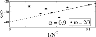
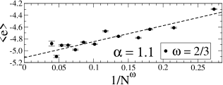
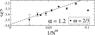
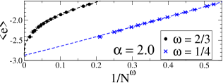
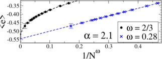
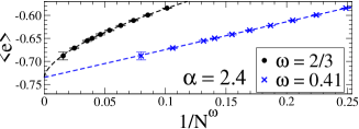
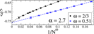
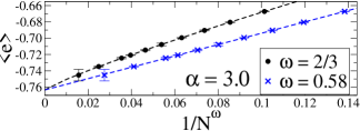
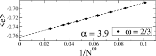
Figure 1: Average ground state energy density $\left\langle e\right\rangle$ obtained with EO for various system sizes up to $N=511$, for values of $\alpha$ between 0.9 and 3.9 in Eq. (1). In each panel, the EO data is once plotted as a function of $1/N^{2/3}$ (black squares), the scaling projected for SK (corresponding to $\alpha\to\infty$), and once linearized with the fitted scaling correction exponent $\omega\left(\alpha\right)$ (blue $\times)$. While no specific scaling can be identified for the smallest $\alpha$, the scaling is consistent with SK (linear on this scale) for larger values of $\alpha$, but significant deviations from $\omega=2/3$ in Eq. (5) are observed for intermediate values of $\alpha$, where $\omega$ appears to attain a minimum of $\omega\approx 0.25$ at $\alpha=2$. The results for $\omega\left(\alpha\right)$ are also summarized in Fig. 4.

IV.1 Corrections to scaling

First, we investigate the average ground state energy density $\left\langle e\right\rangle$ and its finite-size corrections to scaling. In Figs. 1 we plot these energies in an extrapolation plot as a function of inverse system size, $1/N^{2/3}$, which is generally believed to be the magnitude of scaling corrections in the SK. We notice significant deviation from that scaling behavior for varying $\alpha$. For each value of $\alpha$, we have fitted the data to

$$\left\langle e\right\rangle_{N} \sim \left\langle e\right\rangle_{\infty}+\frac{A}{N^{\omega}}.$$ (5)

A plot of the same data but linearized through the scaling in Eq. (5) with the exponent $\omega$ extracted from those fits are also shown in Fig. 1, and the fitted values for $\omega$ as a function of $\alpha$ are displayed in Fig. 4.

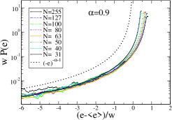
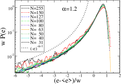
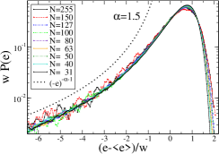
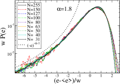
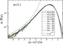
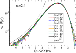
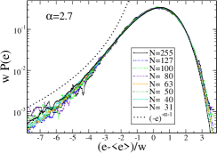
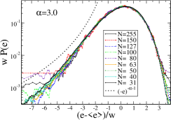
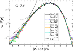
Figure 2: Plot of the ground state energy PDF obtained with EO. We plot the data for all values of $N$ in each panel, whereas $\alpha$ varies between panels from 0.9 to 3.9. The PDFs appear to reach an asymptotic form quickly with small finite-size effects, which are most pronounced for smaller $\alpha$ (and, in fact, are divergent for $\alpha<1$). For $\alpha<2$, the tails for $e\rightarrow-\infty$ are a power-law (dotted lines) with the same exponent as the input bond-distribution $P(J)$ in Eq. (1), since those ground state energies are dominated by a few large bonds that must be satisfied. For $\alpha>2$, the random sum of many small bonds dominates the energy, leading to increasingly exponential tails and the PDF becomes similar to that found in SK (Andreanov et al., 2004; Boettcher, 2005a; Boettcher and Kott, 2005; Palassini, 2008). The scaling of the width $w$ with system size is discussed in Fig. 3.

IV.2 Ground-state energy fluctuations

A deeper insight into the subtleties of ground state energies is provided by their distribution over the ensemble of instances. Typically, we plot the PDF as $\sigma P(e)$ vs. $(e-\left\langle e\right\rangle)/\sigma,$ where $\sigma=\sqrt{\left\langle e^{2}\right\rangle-\left\langle e\right\rangle^{2}}$ is the standard deviation of the distribution. But for $\alpha<2,$ we find that the PDF has a broad tail for energies below the mean, which behaves as $P(e)\sim(-e)^{-\alpha-1}$ for $e\rightarrow-\infty.$ Hence, $\left\langle e^{2}\right\rangle$ and $\sigma$ do not exist. Instead, we define a width via the absolute moment (see Ref. (Press et al., 1995)) $w=\left\langle\left|e-\left\langle e\right\rangle\right|\right\rangle$ to characterize the distribution and plot $wP(e)$ vs. $(e-\left\langle e\right\rangle)/w$ for each $\alpha$ in Figs. 2.

The power-law tails at low energies $e\rightarrow-\infty$ in Figs. 2 for $\alpha<2$ are easy to explain: They are entirely due to those rare, large bonds from deep within the bond distribution in Eq. (1), which almost always must be satisfied and completely dominate the ground state energy when they occur (Newman and Stein, 1994; Cieplak et al., 1994). Accordingly, those tails of the PDF decay with the same exponent, $1+\alpha,$ as Eq. (1).

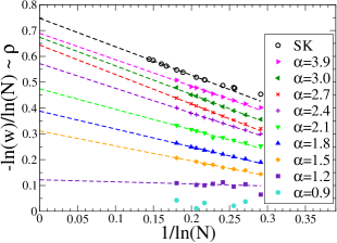
Figure 3: Extrapolation plot of the width $w=\left\langle\left|e-\left\langle e\right\rangle\right|\right\rangle$ of the ground state energy distributions $P(e)$ in Figs. 2 versus system size $N$ for each value of $\alpha$. Note that $\ln(w)/\ln(N)\to-\rho$ for $1/\ln(N)\to 0$. As a reference, we have included the corresponding SK data for $w$ derived from the study in Ref. (Boettcher, 2010a). Theory (Parisi and Rizzo, 2008) provides an upper bound of $\rho=\frac{5}{6}$ that should be approached for large $\alpha$. On the other side, when $\alpha$ drops below 1 the width diverges (in the limit of infinitely many instances), independent of system size $N$, leading to the conclusion $\rho_{\alpha\leq 1}\equiv 0$. For increasing $\alpha>1$, $\rho$ seems to increase rapidly to saturate soon at the SK limit, see Fig. 4.

The feature of $P(e)$ of greatest interest is the scaling of its width. As noted, the standard deviation $\sigma$ does not exist for $\alpha<2$, but we can instead for all $\alpha>1$ refer to the width derived from the first absolute moment, $w=\left\langle\left|e-\left\langle e\right\rangle\right|\right\rangle,$ introduced above. It is expected that, like $\sigma$, the width would decay with system size as

$$w \sim N^{-\rho}.$$ (6)

As an example of the significance of this exponent we mention that according to Ref. (Aspelmeier et al., 2003), $\rho$ is related to the exponent $y$ (or $\theta$) for domain-wall excitations in the large-dimensional limit $d\to\infty$ of the Edwards-Anderson model (Edwards and Anderson, 1975) via

$$y/d=1-\rho,$$ (7)

which has led to much consideration recently (Boettcher, 2005b; Aspelmeier et al., 2008; Parisi and Rizzo, 2008; Aspelmeier, 2008a, b; Parisi and Rizzo, 2010, 2009; Boettcher, 2010a). In Fig. 3, we have plotted the values of $w$ obtained in preparing Fig. 2 as a function of $N$ for each value of $\alpha$. In reference to Eq. (6), we specifically use its extrapolated version and plot $-\ln(w)/\ln(N)$ as a function of $1/\ln(N)$, which should extrapolate linearly to the thermodynamic value of $\rho$ at the intercept $1/\ln(N)\to 0$. It appears that $\rho$ increases from zero at $\alpha\leq 1$ to saturate at the SK value. Although large uncertainties in the precise value of $\rho$ for each individual $\alpha$ should be expected (and possibly non-analyticities or logarithmic corrections), the general trend in $\rho$ appears to be reliable. The SK data provides justification for choosing $w$ as the width instead of the more conventional deviation $\sigma$: The extrapolation of $w$ in Fig. 3 leads to identical results for $\sigma$ as in Refs. (Boettcher, 2005a, 2010a).

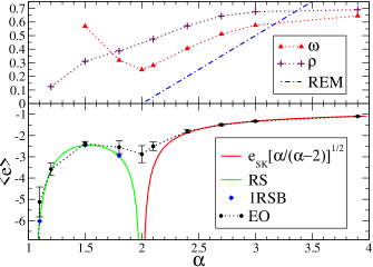
Figure 4: Top panel: Plot of the measured values of the exponents $\omega$ (from Figs. 1) and $\rho$ (from Fig. 3) over the range of values for $\alpha$ used in this study. (Lines are added just to guide the eye.) For $\alpha>1$, $\omega$ initially drops towards a minimum near $\alpha=2$ to rise again and approach its SK-value of 2/3. In turn, $\rho$ rises monotonically from about zero at $\alpha=1$ to its SK-value, which is which varies only little for $\alpha\geq 3$. The dash-dotted line corresponds to the naive REM calculation, see Eq. (29). Bottom panel: Plot of the ground state energy densities in the scaling of Eq. (3). Black circles denote the extrapolated EO values found in Fig. 1 (connected by a dotted line to guide the eye). The line for $1<\alpha<2$ corresponds to the RS- and the blue diamonds to the 1RSB-calculation from Ref. (Janzen et al., 2010a, b), the line for $\alpha>2$ provides the exact SK-energy $e_{SK}=-0.76321\ldots$, appropriately rescaled. The energies found with EO deviate significantly from the theoretical values near $\alpha=2$, where finite-size corrections are also the strongest (or, $\omega$ is minimal, see top).

IV.3 Exponents as a function of $\alpha$ for $2<\alpha<4$

While $\rho$ appears to rise rapidly but monotonously from zero at $\alpha=1$ to approach the SK-limit, $\omega$ instead has a distinct minimum of about $\omega\approx 0.25$ near $\alpha=2$. For larger $\alpha$, it approaches the presumed SK-value of $\omega=2/3$. In turn, in the limit for $\alpha\to 1^{-}$, $\omega$ may revert to its SK value, although a simple volume-size correction to the energy with $\omega=1$ or even exponentially small size corrections with $\omega\to\infty$ appear conceivable. Although both exponents, $\omega$ and $\rho$, approach the corresponding SK-value convincingly for larger values of $\alpha$, that limit is attained in a manner that requires some explanation. Even for values of $\alpha>2$, where a second moment in $P(J)$ already exists, both exponents still deviate significantly from their SK-values. The smallest value beyond which one might argue that the SK-limit has been saturated would be $\alpha=3$, but it may even be higher. Our data would indicate a steady approach to that limit but its system-size limitations certainly could not exclude a singular “bend” at $\alpha=3$, say.

We argue that the origin of these anomalous exponents for $\alpha>2$ can be tied to higher-order differences between the moments of a Gaussian and a Levy distribution. In particular, for $\alpha\leq 4$, the 4th moment of the Levy distribution remains divergent. As both exponents refer to finite-size effects, i.e., they do not per-se relate to properties of the SK (that are universal for $2<\alpha<4$) in the thermodynamic limit, the sensitivity of these exponents to such differences is not surprising. In the Appendix, we have done a speculative calculation for the finite-size scaling corrections in the REM model (Derrida, 1980, 1981) with Levy bonds. The key result, Eq. (29), clearly demonstrates that at this level there are anomalous scaling exponents already for $2<\alpha<4$, well in qualitative accord with our numerical findings in Fig. 4, where we indicated the REM result by a dash-dotted line.

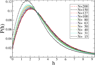
Figure 5: Plot of the distribution of local fields $P(h)$ for $h\geq 0$ only for a range of system sizes $N$. (The function is symmetric, and it is normalized to 1/2 for the positive part shown here.) The distribution is nearly linear for $h\to 0$, although higher order terms become more noticeable for increasing $h$ than is the case for SK (Boettcher et al., 2008). For larger values of $h$, we observe a much broader tail than for SK, yet, that tail still represents an exponential fall-off. From this plot it is not clear whether $P(h)$ at $h=0$ remains finite for $N\to\infty$, therefore, we study the behavior of $P(0)$ more closely in Fig. 6.

IV.4 Local field distribution at $\alpha=3/2$

We now investigate also the distribution of local fields $P(h)$ in the ground state configurations for $\alpha=3/2$. Instead of parsing out the whole parameter space, we focus on a single value of $\alpha$ to optimize statistics. Specifically, $\alpha=3/2$ is chosen, since it is ideally located sufficiently below the cross-over regime near $\alpha=2$ , above which the central limit theorem comes into play, and sufficiently above $\alpha=1$, where (numerical and theoretical) pathologies arise due to the extreme breadth of the bond distribution.

In Fig. 5 we plot the data obtained for $P(h)$ for $\alpha=3/2$ up to $N=200$. The function has similar characteristics to those observed in other spin glasses (Boettcher et al., 2008), with a near-Poissonian shape, but with a much broader tail for larger $h$. Overall, at $N=200$ finite-size effects have largely diminished already, with the notable exception near $h=0$, which in turn harbors the dynamically most relevant information contained in $P(h)$. In the ground state configuration (in which almost all variables have a positive local field) the number of variables with near-vanishing local field characterize the stability of the state, for which the scaling-behavior of $P(h)$ for $N\to\infty$ and $h\to 0$ holds the key. Despite significant curvature for increasing $h$, it seems clear from Fig. 5 that the slope of $P(h)$ is nonetheless linear at the origin, as it is for SK.

To obtain a closer insight into the scaling of $P(0)$ itself, we plot in Fig. 6 just the values at the origin of Fig. 5 as a function of system size $N$. It is very hard to get well-converged data for larger system sizes, such as those available for SK (Boettcher et al., 2008), but luckily the data exhibits already solid scaling starting with $N\geq 31$. The scaling, with an exponent of about $\approx 0.4$, indicates that $P(0)\to 0$ in the thermodynamic limit but is definitely slower decaying than for SK, which falls with $1/\sqrt{N}$ (Boettcher et al., 2008).

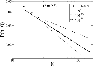
Figure 6: Plot of $P(0)$ as a function of system size $N$. The data exhibits scaling over almost a decade, decaying roughly as $N^{-0.39}$, displayed as the full line. For comparison, lines for a $N^{-1/2}$ (dotted line) and $N^{-1/4}$-decay (dash-dotted line) are also plotted.

V Acknowledgments

Many thanks to J-P. Bouchaud for his suggestions that initiated this project. I am greatly indebted to K. Janzen and A. Engel for many clarifying discussion and for providing me with some of their data, and to the Fulbright Kommission for supporting my stay at Oldenburg University. This work has been supported also by grants 0312510 and 0812204 from the Division of Materials Research at the National Science Foundation and by the Emory University Research Council.

VI Appendix: Finite-Size Corrections in the Levy-REM

We use here the assumption of the random energy model (REM) (Derrida, 1980, 1981) that the spectrum of available states are uncorrelated to obtain an estimate for the finite-size scaling of the SK model with Levy bonds. This is true for the $p$-spin generalization of SK in the limit of $p\to\infty$ with Gaussian bonds, but this is clearly not obvious for Levy bonds. We go even further and assume this to hold even for $p=2$, the case considered for SK in this paper, in order to estimate leading-order scaling and finite-size corrections to the ground state energy density. A full treatment of the Levy-REM would likely be a lengthy exercise but potentially rewarding as interesting classes of the extreme-value distribution of ground-state energies and of the local field distribution may result.

VI.1 REM with Gaussian bonds

To review the REM(Derrida, 1980, 1981; Gross and Mezard, 1984) calculation for the Hamiltonian of the $p$-spin model,

$${\cal H}\left(\left\{\sigma_{i}\right\}\right) = \frac{1}{p!}\sum_{i_{1}=1,\ldots,i_{p}=1}^{N}J_{i_{1},\ldots,i_{p}}\sigma_{i_{1}}\times\ldots\times\sigma_{i_{p}},$$ (8)

for Gaussian bonds, we set

$$P\left(J\right) = \sqrt{\frac{N^{p-1}}{\pi p!}}\exp\left\{-\frac{N^{p-1}}{p!}J^{2}\right\}$$ (9)

and, following Ref. (Fischer and Hertz, 1991), calculate the densities of energy-levels via

$${\cal D}\left(E\right)=\left\langle\delta\left(E-{\cal H}\left(\left\{\sigma_{i}\right\}\right)\right)\right\rangle_{J},$$ (10)

$$=\int\prod_{i_{1},\ldots,i_{p}}^{N}\left[dJ_{i_{1},\ldots,i_{p}}P\left(J_{i_{1},\ldots,i_{p}}\right)\right]$$

$$\qquad\delta\left(E-\frac{1}{p!}\sum_{i_{1},\ldots,i_{p}}^{N}J_{i_{1},\ldots,i_{p}}\sigma_{i_{1}}\ldots\sigma_{i_{p}}\right),$$

$$=\int_{-\infty}^{\infty}\frac{dt}{2\pi}\,e^{iEt}\prod_{i_{1}=1,\ldots,i_{p}=1}^{N}\left[\int dJP\left(J\right)\exp\left\{\frac{iJt}{p!}\sigma_{i_{1}}\ldots\sigma_{i_{p}}\right\}\right],$$

assuming in the first line that the energies are uncorrelated:

$${\cal D}\left(E_{1},E_{2}\right)={\cal D}\left(E_{1}\right){\cal D}\left(E_{2}\right).$$ (11)

The ensuing Gaussian integral in Eq. (10) only depends on $\left(\sigma_{i_{1}}\ldots\sigma_{i_{p}}\right)^{2}\equiv 1$, thus,

$${\cal D}\left(E\right)=\int_{-\infty}^{\infty}\frac{dt}{2\pi}e^{N\psi\left(t\right)}$$ (12)

with

$$\psi\left(t\right)=it\frac{E}{N}-\frac{t^{2}}{4}.$$ (13)

Of course, no steepest-descent analysis is required here to solve this integral:

$${\cal D}\left(E\right) = \frac{e^{-\frac{E}{N}^{2}}}{\sqrt{N\pi}}.$$ (14)

Then, we get for the entropy

$$S\left(E\right) = \ln\Omega\left(E\right)=\ln\left[2^{N}{\cal D}\left(E\right)\right]$$ (15)

$$= N\left[\ln 2-\left(\frac{E}{N}\right)^{2}+O\left(\frac{\ln N}{N}\right)\right].$$

As the entropy may not become negative, vanishing of the entropy (-density) defines the ground-state energy density

$$\frac{E_{0}}{N} = -\sqrt{\ln 2}+O\left(\frac{\ln N}{N}\right).$$ (16)

Its numerical value, $-\sqrt{\ln 2}=-0.832555$, is plausible when compared to the Parisi energy, $e_{SK}=-0.763217\ldots$ (Oppermann and Sherrington, 2005; Oppermann et al., 2007). The implicated finite-size correction of this result, $\ln\left(N\right)/N$ or $\omega=1$, of course, does not correspond to the SK result for $p=2$, presumed to scale with $N^{-\frac{2}{3}}$. But since this result has become entirely independent of $p\geq 2$, one would hardly expect a better agreement. After all, only for $p\to\infty$ are these energy levels sufficiently uncorrelated, as in Eq. (11), to justify this approach. The value of our calculation here lies not so much in a precise prediction for $\omega$ but in a plausible trend in the function $\omega(\alpha)$ and its transitions.

VI.2 REM with Levy Bonds

We can repeat the above calculation for the $p$-spin Hamiltonian in Eq. (8) with a bond distribution of the Levy-type,

$$P\left(J\right) = \frac{\alpha}{2}B^{\alpha}\left|J\right|^{-1-\alpha}\theta\left(\left|J\right|-B\right),$$ (17)

for some positive $B$, which will be discussed below.

Inserting this bond distribution into Eq. (10) results in a density of states ${\cal D}\left(E\right)$ as in Eq. (12) using

$$\psi\left(t\right)=\pm it\frac{E}{N}+N^{p-1}\ln\left[f_{\alpha}\left(\frac{tB}{p!}\right)\right]$$ (18)

with

$$f_{\alpha}\left(x\right)=\alpha\int_{1}^{\infty}d\xi\frac{\cos\left[x\xi\right]}{\xi^{1+\alpha}},$$ (19)

which can be written in terms of special functions to facilitate the ensuing analysis:

$$f_{\alpha}\left(x\right) = \,{}_{1}F_{2}\left(-\frac{\alpha}{2};\frac{1}{2},1-\frac{\alpha}{2};-\frac{x^{2}}{4}\right)$$ (20)

$$\quad-\cos\left(\frac{\pi}{2}\alpha\right)\Gamma\left(1-\alpha\right)x^{\alpha}.$$

For even $\alpha=2,4,\ldots$, both terms in Eq. (20) develop identical singularities for small $x$ in a way that the resulting expression always remains finite:

$$f_{2}\left(x\right) = \cos\left(x\right)-x\sin\left(x\right)+x^{2}{\rm Ci}\left(x\right),$$ (21)

$$f_{4}\left(x\right) = \left(1-\frac{x^{2}}{6}\right)\cos\left(x\right)$$

$$\quad-\frac{x}{6}\left(2-x^{2}\right)\sin\left(x\right)-\frac{x^{4}}{6}{\rm Ci}\left(x\right).$$

From Eq. (18) it is clear that for the saddle point in the thermodynamic limit $N\to\infty$, $B$ will have to be chosen to scale with the system size as to make $\psi\left(t\right)$ stationary in that limit and to render the energy density $E/N$ intensive, i. e., it has to serve to compensate the explicit factor of $N^{p-1}$. We expect that for all values of $\alpha$ the saddle point is located at some (possibly complex) finite value of $t_{0}$ while $B$ becomes small in some fashion for $N\to\infty$. In that case, we are merely looking for the series expansion of $\ln\left[f_{\alpha}\left(x\right)\right]$ for small values of $x$:

$$-\ln f_{\alpha}\left(x\right) \sim \cos\left(\frac{\pi}{2}\alpha\right)\Gamma\left(1-\alpha\right)x^{\alpha}+\frac{\alpha}{2\left(\alpha-2\right)}x^{2}$$ (22)

$$\quad+\frac{\alpha\left(\alpha^{2}-4\alpha-2\right)}{12\left(\alpha-4\right)\left(\alpha-2\right)^{2}}x^{4}+\ldots,$$

as long as $\alpha>2$; for $\alpha<2$ there are higher powers of the $x^{\alpha}$-term in Eq. (20) from the expansion of the logarithm to take into account. There are exceptional cases for $\alpha=2,4,\ldots$:

$$\ln f_{2}\left(x\right) \sim x^{2}\left[\left(\ln x+\gamma\right)-\frac{3}{2}\right]$$

$$-\frac{x^{4}}{6}\left[3\left(\ln x+\gamma\right)^{2}-9\left(\ln x+\gamma\right)+7\right]+\ldots,$$

$$\ln f_{4}\left(x\right) \sim -x^{2}-\frac{x^{4}}{72}\left[12\left(\ln x+\gamma\right)+11\right]+\ldots.$$ (23)

Case $\alpha>4$:

For $\alpha>4$, the irregular term in Eq. (22) becomes irrelevant for the determination of ground-state energy density and its corrections. We find for $\psi\left(t\right)$ in Eq. (18) to leading orders,

$$\psi\left(t\right) \sim it\frac{E}{N}-\frac{\alpha}{2\left(\alpha-2\right)}N^{p-1}\left(\frac{tB}{p!}\right)^{2}$$ (24)

$$-\frac{\alpha\left(\alpha^{2}-4\alpha-2\right)}{12\left(\alpha-4\right)\left(\alpha-2\right)^{2}}N^{p-1}\left(\frac{tB}{p!}\right)^{4}+\ldots,$$

$$\sim it\frac{E}{N}-\frac{t}{4}^{2}+C\frac{t^{4}}{N^{p-1}}+\ldots,$$

for some constant $C$ and with the choice of

$$B = \sqrt{\frac{p!\left(\alpha-2\right)}{2\alpha}}\,N^{-\frac{p-1}{2}}.$$ (25)

We can write the density of states in Eq. (12) as

$${\cal D}\left(E\right) \sim \int_{-\infty}^{\infty}\frac{dt}{2\pi}\,e^{N\left(it\frac{E}{N}-\frac{t}{4}^{2}\right)+C\frac{t^{4}}{N^{p-2}}+\ldots}.$$ (26)

Focusing only on a small $\epsilon$-neighborhood in $t$ near the saddle-point $t_{0}=2i\frac{E}{N}$ (with $1/\sqrt{N}\ll\epsilon\ll 1$), followed by the shift $t=t_{0}+\frac{u}{\sqrt{N}}$ yields (Bender and Orszag, 1978)

$${\cal D}\left(E\right) \sim \frac{e^{-N\left[\left(\frac{E}{N}\right)^{2}+O\left(\frac{1}{N^{p-1}}\right)\right]}}{\sqrt{\pi N}}$$

$$\quad\int_{-\epsilon\sqrt{N}\to-\infty}^{\epsilon\sqrt{N}\to\infty}\frac{du}{\sqrt{4\pi}}\,\left[1+O\left(\frac{u^{2}}{N^{p-1}}\right)\right]e^{-\frac{u^{2}}{4}},$$

$$\sim \exp\left\{-N\left[\left(\frac{E}{N}\right)^{2}+O\left(\frac{\ln N}{N}\right)+O\left(\frac{1}{N^{p-1}}\right)\right]\right\}.$$

Hence, for $\alpha>4$ there is neither a change in scaling for the leading-order calculation for the ground state energy density nor for its finite size correction from those obtained for the REM with Gaussian bonds in Sec. VI.1, as for $p=2$ (or larger) any corrections arising from the broader tails remain sub-dominant. Furthermore, the pre-factor in the choice of $B$ in Eq. (25) ensures that the second moment of the bond distribution remains unity, $\left\langle J^{2}\right\rangle=1$, for all $\alpha>2$, such that the ground-state energy is also numerically identical to that of the Gaussian case.

Case $2<\alpha<4$:

In this case, the irregular term in Eq. (22) now becomes relevant for the determination of the finite-size correction for the ground-state energy density and its corrections. With the same choice of $B$ as in Eq. (25), we then find for $\psi\left(t\right)$ in Eq. (18) to leading orders,

$$\psi\left(t\right) \sim it\frac{E}{N}-\frac{\alpha}{2\left(\alpha-2\right)}N^{p-1}\left(\frac{tB}{p!}\right)^{2}$$ (28)

$$\leavevmode\nobreak\ \leavevmode\nobreak\ +\cos\left(\frac{\pi}{2}\alpha\right)\Gamma\left(1-\alpha\right)N^{p-1}\left(\frac{tB}{p!}\right)^{\alpha}+\ldots,$$

$$\sim it\frac{E}{N}-\frac{t}{4}^{2}+C\frac{t^{\alpha}}{N^{\left(\frac{\alpha}{2}-1\right)\left(p-1\right)}}+\ldots.$$

Following exactly along the lines of Eqs. (26-VI.2), we obtain

$$-\frac{\ln{\cal D}\left(E\right)}{N}\sim\left(\frac{E}{N}\right)^{2}+O\left(\frac{\ln N}{N}\right)+O\left(\frac{1}{N^{\left(\frac{\alpha}{2}-1\right)\left(p-1\right)}}\right),$$

where now the correction in $\psi(t)$ accounts for the next-to-leading term, dominating the factor originating from the Gaussian saddle-point integral for some ($p>2$) or all ($p=2$) of this regime. We surmise that to leading order we retain the ground-state energy from the Gaussian case here (as the second moment of the bond distribution still exists!), but already in this regime of $\alpha$ we find a non-universal effect in terms of the finite-size corrections (Boettcher, 2010b). For instance, ignoring the fact that statistical independence of the energy levels only holds for $p\to\infty$, we boldly set $p=2$ to extract an approximation for the finite-size scaling exponent,

$$\omega(\alpha) = \frac{\alpha}{2}-1\qquad\left(2<\alpha<4\right).$$ (29)

While not in great quantitative agreement with the numerical results for $p=2$, this analysis does indeed capture the essence of the numerical results to some qualitative satisfaction.

Case $\alpha=2$:

It seems clear that in this case not only the corrections but also the ground state itself will pick up some messy form of log-scaling. To this end, it suffices to determine the form of $B$ that leaves the saddle-point stationary for $N\to\infty$. From Eqs. (18) and expanding (23) to sufficient order, we get

$$\psi\left(t\right) \sim it\frac{E}{N}+N^{p-1}\left(\frac{tB}{p!}\right)^{2}\ln\left(\frac{tB}{p!}\right)+\ldots.$$ (30)

Even for general complex $t$, the saddle-point is still determined via $\psi^{\prime}\left(t_{0}\right)=0$. The obtained saddle-point at

$$t_{0} \sim i\left(\frac{E}{N}\right)\frac{\left(p!\right)^{2}}{2N^{p-1}B^{2}\ln\left(N^{p-1}B\right)}$$ (31)

becomes stationary for the choice of

$$B = \frac{1}{N^{\frac{p-1}{2}}\sqrt{\ln N^{\frac{p-1}{2}}}}.$$ (32)

Thus, we have acquired an unusual logarithmic correction, already for the leading behavior of the ground state energy density. Inserting $t_{0}$ in Eq. (31) into $\psi\left(t\right)$ in Eq. (30) yields

$$\psi\left(t_{0}\right) = -\frac{\left(p!\right)^{2}}{4}\left(\frac{E}{N}\right)^{2}\left[1+O\left(\frac{\ln\sqrt{\ln N^{\frac{p-1}{2}}}}{\ln N^{\frac{p-1}{2}}}\right)\right],$$ (33)

assuming that any other contribution from the actual saddle-point integral only results in much smaller corrections than the indicated ones, arising from the corrections in the motion of the saddle-point itself. At $p=2$, we would therefore predict for the ground state energy density,

$$\frac{E_{0}}{N} = -\sqrt{\ln 2}+O\left(\frac{\ln\sqrt{\ln\sqrt{N}}}{\ln\sqrt{N}}\right),$$ (34)

with the same thermodynamic limit as before, but much smaller corrections. Of course, such a scaling is nearly impossible to verify numerically.

Case $1<\alpha<2$:

Now, the saddle-point analysis changes somewhat, with the integration contour being rotated into the complex plane, requiring a more sophisticated steepest-descent approach (Bender and Orszag, 1978). In our naive approach taken here, we find that reasonable solutions for $E_{0}$ persist for $\alpha>\frac{3}{2}$, at which point the saddle point rotates across the branch-cut on the negative real-axis in the complex-$t$ plane. We leave this calculation as an exercise for the reader.

References

- Sherrington and Kirkpatrick (1975) D. Sherrington and S. Kirkpatrick, Phys. Rev. Lett. 35, 1792 (1975).
- Mézard et al. (1987) M. Mézard, G. Parisi, and M. A. Virasoro, Spin glass theory and beyond (World Scientific, Singapore, 1987).
- Fischer and Hertz (1991) K. H. Fischer and J. A. Hertz, Spin Glasses (Cambridge University Press, Cambridge, 1991).
- Nishimori (2001) H. Nishimori, Statistical Physics of Spin Glasses and Information Processing (Oxford University, Oxford, 2001).
- Mezard et al. (2002) M. Mezard, G. Parisi, and R. Zecchina, Science 297, 812 (2002).
- Talagrand (2003) M. Talagrand, Spin Glasses: Cavity and Mean Field Models (Springer, Berlin, 2003).
- Eastham et al. (2006) P. R. Eastham, R. A. Blythe, A. J. Bray, and M. A. Moore, Phys. Rev. B 74, 020406(R) (2006).
- Schneidman et al. (2006) E. Schneidman, M. J. Berry, R. Segev, and W. Bialek, Nature 440, 1007 (2006).
- Percus et al. (2006) A. Percus, G. Istrate, and C. Moore, Computational Complexity and Statistical Physics (Oxford University Press, New York, 2006).
- Mézard and Montanari (2006) M. Mézard and A. Montanari, Constraint Satisfaction Networks in Physics and Computation (Oxford University Press, Oxford, 2006).
- Bouchaud et al. (2003) J.-P. Bouchaud, F. Krzakala, and O. C. Martin, Phys. Rev. B 68, 224404 (2003).
- Aspelmeier et al. (2003) T. Aspelmeier, M. A. Moore, and A. P. Young, Phys. Rev. Lett. 90, 127202 (2003).
- Andreanov et al. (2004) A. Andreanov, F. Barbieri, and O. C. Martin, Eur. Phys. J. B 41, 365 (2004).
- Boettcher (2005a) S. Boettcher, Eur. Phys. J. B 46, 501 (2005a).
- Aspelmeier et al. (2008) T. Aspelmeier, A. Billoire, E. Marinari, and M. A. Moore, J. Phys. A: Math. Theor. 41, 324008 (2008).
- Palassini (2008) M. Palassini, J. Stat. Mech. P10005 (2008).
- Boettcher (2010a) S. Boettcher, J. Stat. Mech P07002 (2010a).
- Boettcher (2010b) S. Boettcher, Euro. Phys. J. B 74, 363 (2010b).
- Edwards and Anderson (1975) S. F. Edwards and P. W. Anderson, J. Phys. F 5, 965 (1975).
- Boettcher (2005b) S. Boettcher, Phys. Rev. Lett. 95, 197205 (2005b).
- Cizeau and Bouchaud (1993) P. Cizeau and J. P. Bouchaud, J. Phys. A: Math. Gen. 26, L187 (1993).
- Janzen et al. (2008) K. Janzen, A. K. Hartmann, and A. Engel, J. Stat. Mech. P04006 (2008).
- Janzen et al. (2010a) K. Janzen, A. Engel, and M. Mezard, EuroPhys. Lett. 89, 67002 (2010a).
- Janzen et al. (2010b) K. Janzen, A. Engel, and M. Mézard, Phys. Rev. E 82, 021127 (2010b).
- Neri et al. (2010) I. Neri, F. L. Metz, and D. Bollé, J. Stat. Mech. P01010 (2010).
- Newman and Stein (1994) C. M. Newman and D. L. Stein, Phys. Rev. Lett. 72, 2286 (1994).
- Cieplak et al. (1994) M. Cieplak, A. Maritan, and J. R. Banavar, Phys. Rev. Lett. 72, 2320 (1994).
- Boettcher and Percus (2001) S. Boettcher and A. G. Percus, Phys. Rev. Lett. 86, 5211 (2001).
- Hartmann and Rieger (2004) A. Hartmann and H. Rieger, eds., New Optimization Algorithms in Physics (Wiley-VCH, Berlin, 2004).
- Zdeborova and Boettcher (2010) L. Zdeborova and S. Boettcher, J. Stat. Mech. P02020 (2010).
- Derrida (1980) B. Derrida, Phys. Rev. Lett. 45, 79 (1980).
- Derrida (1981) B. Derrida, Phys. Rev. B 24, 2613 (1981).
- Oppermann and Sherrington (2005) R. Oppermann and D. Sherrington, Phys. Rev. Lett. 95, 197203 (2005).
- Oppermann et al. (2007) R. Oppermann, M. J. Schmidt, and D. Sherrington, Phys. Rev. Lett. 98, 127201 (2007).
- Boettcher and Percus (2000) S. Boettcher and A. G. Percus, Artificial Intelligence 119, 275 (2000).
- Boettcher and Davidheiser (2008) S. Boettcher and J. Davidheiser, Phys. Rev. B 77, 214432 (2008).
- Boettcher and Kott (2005) S. Boettcher and T. M. Kott, Phys. Rev. B 72, 212408 (2005).
- Press et al. (1995) W. H. Press, S. A. Teukolsky, W. T. Vetterling, and B. P. Flannery, Numerical Recipes in C (Cambridge University Press, Cambridge, 1995).
- Parisi and Rizzo (2008) G. Parisi and T. Rizzo, Phys. Rev. Lett. 101, 117205 (2008).
- Aspelmeier (2008a) T. Aspelmeier, J. Stat. Mech. P04018 (2008a).
- Aspelmeier (2008b) T. Aspelmeier, Phys. Rev. Lett. 100, 117205 (2008b).
- Parisi and Rizzo (2010) G. Parisi and T. Rizzo, J. Phys. A: Math. Theor. 43, 045001 (2010).
- Parisi and Rizzo (2009) G. Parisi and T. Rizzo, Phys. Rev. B 79, 134205 (pages 12) (2009).
- Boettcher et al. (2008) S. Boettcher, H. G. Katzgraber, and D. Sherrington, J. Phys. A: Math. Theor. 41, 324007 (2008).
- Gross and Mezard (1984) D. J. Gross and M. Mezard, Nucl. Phys. B 240, 431 (1984).
- Bender and Orszag (1978) C. M. Bender and S. A. Orszag, Advanced Mathematical Methods for Scientists and Engineers (McGraw-Hill, New York, 1978).