Self-similar solutions of the three dimensional Navier-Stokes equation

Abstract

In this article we will present pure three dimensional analytic solutions for the Navier-Stokes and the continuity equations in Cartesian coordinates. The key idea is the three-dimensional generalization of the well-known self-similar Ansatz of Barenblatt. A geometrical interpretation of the Ansatz is given also. The results are the Kummer functions or strongly related. Our final formula is compared with other results obtained from group theoretical approaches.

To describe the dynamics of viscous incompressible fluids the Navier-Stokes (NS) partial differential equation (PDE) together with the continuity equation have to be investigated. In Cartesian coordinates and Eulerian description these equations have the following form:

$${\bf{\nabla}}{\bf{v}}=0,$$

$${\bf{v}}_{t}+({\bf{v}}\nabla){\bf{v}}=\nu\triangle{\bf{v}}-\frac{\nabla p}{\rho}+a$$ (1)

where ${\bf{v}},\rho,p,\nu,a$ denote respectively the three-dimensional velocity field, density, pressure, kinematic viscosity and an external force (like gravitation) of the investigated fluid. (To avoid further misunderstanding we use $a$ for external field instead of the letter g which is reserved for a self-similar solution.) In the following $\nu,a$ are parameters of the flow. For a better transparency in the following we use the coordinate notation ${\bf{v}}(x,y,z,t)=u(x,y,z,t),v(x,y,z,t),w(x,y,z,t)$ and for the scalar pressure variable $p(x,y,z,t)$

$$u_{x}+v_{y}+w_{z}=0$$

$$u_{t}+uu_{x}+vu_{y}+wu_{z}=\nu(u_{xx}+u_{yy}+u_{zz})-\frac{p_{x}}{\rho}$$

$$v_{t}+uv_{x}+vv_{y}+wv_{z}=\nu(v_{xx}+v_{yy}+v_{zz})-\frac{p_{y}}{\rho}$$

$$w_{t}+uw_{x}+vw_{y}+ww_{z}=\nu(w_{xx}+w_{yy}+w_{zz})-\frac{p_{z}}{\rho}+a.$$ (2)

The subscripts mean partial derivations. According to our best knowledge there are no analytic solution for the most general three dimensional case. However, there are various examination techniques available in the literature. Manwai manwai studied the N-dimensional $(N\geq 1)$ radial Navier-Stokes equation with different kind of viscosity and pressure dependences and presented analytical blow up solutions. His works are still 1+1 dimensional (one spatial and one time dimension) investigations. Another well established and popular investigation method is based on Lie algebra there are numerous studies available. Some of them are even for the three dimensional case, for more see lie . Unfortunately, no explicit solutions are shown and analyzed there. Fushchich et al. fus construct a complete set of ${\tilde{G}}(1,3)$-inequivalent Ansätze of codimension 1 for the NS system, they present 19 different analytical solutions for one or two space dimensions. They last solution is very closed to our one but not identical, we will come back to these results later. Further two and three dimensional studies based on group analytical method were presented by Grassi grassi . They also present solutions which look almost the same as ours, but they consider only 2 space dimensions. We will compare these results to our one at the end of the paper.

Recently, Hu et al. hu presents a study where symmetry reductions and exact solutions of the (2+1)-dimensional NS were presented. Aristov and Polyanin arist use various methods like Crocco transformation, generalized separation of variables or the method of functional separation of variables for the NS and present large number of new classes of exact solutions. Sedov in his classical work sedov * presented analytic solutions for the tree dimensional spherical NS equation where all three velocity components and the pressure have polar angle dependence ($\theta$) only. Even this kind of restricted symmetry led to a non-linear coupled ordinary differential equation system with has a very rich mathematical structure.

Beyond the NS system there are other important and popular PDEs which attract much interest and investigation. The applied methods are the same there, too. Without completeness we mention some examples. For one dimensional cubic-quintic nonlinear Schrödinger equation a quite general self-similar type of solution $\psi(z,t)=u(z,t)exp[iv(z,t)]$ was applied where u and v are real functions wu . The results are analytic solutions for an external potential with variable coefficients. A more general type of this Ansatz $u(z,t)=A(z)U[T(z,t)exp(i\varphi(z,t))]$ was used with success to get chirped and chirp-free self-similar cnoidal solitary wave solutions dai for the same equation. Such solutions can be generalized for multi dimensional spatial coordinates. There are analytic solitary wave solutions available for the (3+1) dimensional Gross-Pitaevskii equation with the following Ansatz $\psi=u(x,y,z,t)R(t)exp[ib(t)(x^{2}+y^{2}+z^{2})]$ gao .

From basic textbooks the form of the one-dimensional self-similar Ansatz is well-known sedov ; barenb ; zeld

$$T(x,t)=t^{-\alpha}f\left(\frac{x}{t^{\beta}}\right):=t^{-\alpha}f(\eta),$$ (3)

where $T(x,t)$ can be an arbitrary variable of a PDE and $t$ means time and $x$ means spatial dependence. The similarity exponents $\alpha$ and $\beta$ are of primary physical importance since $\alpha$ represents the rate of decay of the magnitude $T(x,t)$, while $\beta$ is the rate of spread (or contraction if $\beta<0$ ) of the space distribution as time goes on. The most powerful result of this Ansatz is the fundamental or Gaussian solution of the Fourier heat conduction equation (or for Fick’s diffusion equation) with $\alpha=\beta=1/2$. These solutions are visualized on figure 1. for time-points $t_{1}<t_{2}$. In the pioneering work of Leray leray in 1934 at the end of the manuscript he asks whether it is possible to construct self-similar solutions to the NS system in ${\bf{R}}^{3}$ in the form of $p(x,t)=\frac{1}{T-1}P(x/\sqrt{T-t})$ and ${\bf{v}}(x,t)=\frac{1}{\sqrt{T-t}}{\bf{V}}(x/{\sqrt{T-t}})$. In 2001 Miller et al. miller proof the nonexistence of singular pseudo-self-similar solutions of the NS system with such kind of solutions. Unfortunately, there is no direct analytic calculation with the 3 dimensional self-similar generalization of this Ansatz in the literature. We will show later on that in our case the time dependence has the same exponents as showed above.

Applicability of this Ansatz is quite wide and comes up in various transport systems sedov ; barenb ; zeld ; kers ; barn ; barna2 .

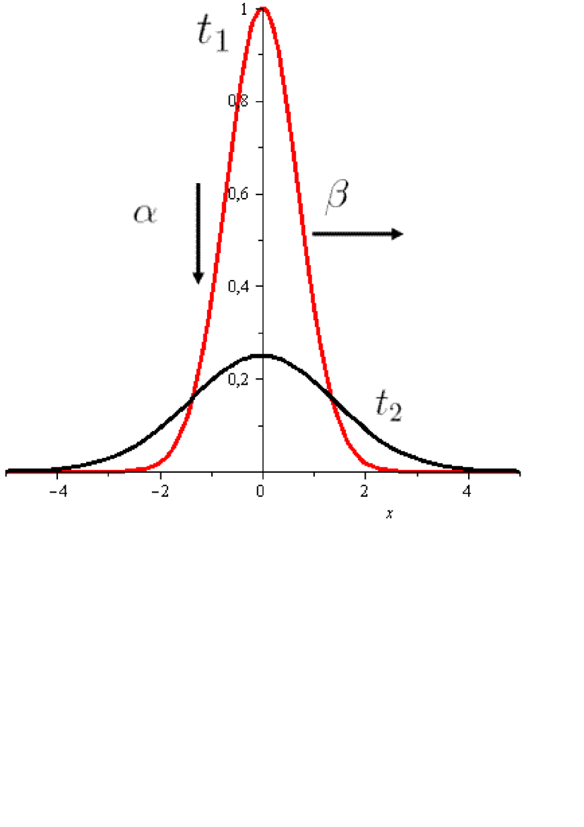
Figure 1: A self-similar solution of Eq. (3) for $t_{1}<t_{2}$. The presented curves are Gaussians for regular heat conduction.

This Ansatz can be generalized for two or three dimensions in various ways one is the following

$$u(x,y,z,t)=t^{-\alpha}f\left(\frac{F(x,y,z)}{t^{\beta}}\right):=t^{-\alpha}f\left(\frac{x+y+z}{t^{\beta}}\right):=t^{-\alpha}f(\omega)$$ (4)

where $F(x,y,z)$ can be understood as an implicit parameterization of a two dimensional surface. If the function $F(x,y,z)=x+y+z=0$ which is presented on figure 2. then it is an implicit form of a plane in three dimensions. At this point we can give a geometrical interpretation of the Ansatz. Note that the dimension of $F(x,y,z)$ still have to be a spatial coordinate. With this Ansatz we consider all the x coordinate of the velocity field ${\bf{v}_{x}}=u$ where the sum of the spatial coordinates are on a plane on the same footing. We are not considering all the $R^{3}$ velocity field but a plane of the ${\bf{v}}_{x}$ coordinates as an independent variable. The Navier-Stokes equation - which is responsible for the dynamics - maps this kind of velocities which are on a surface to another geometry. In this sense we can investigate the dynamical properties of the NS equation truly.

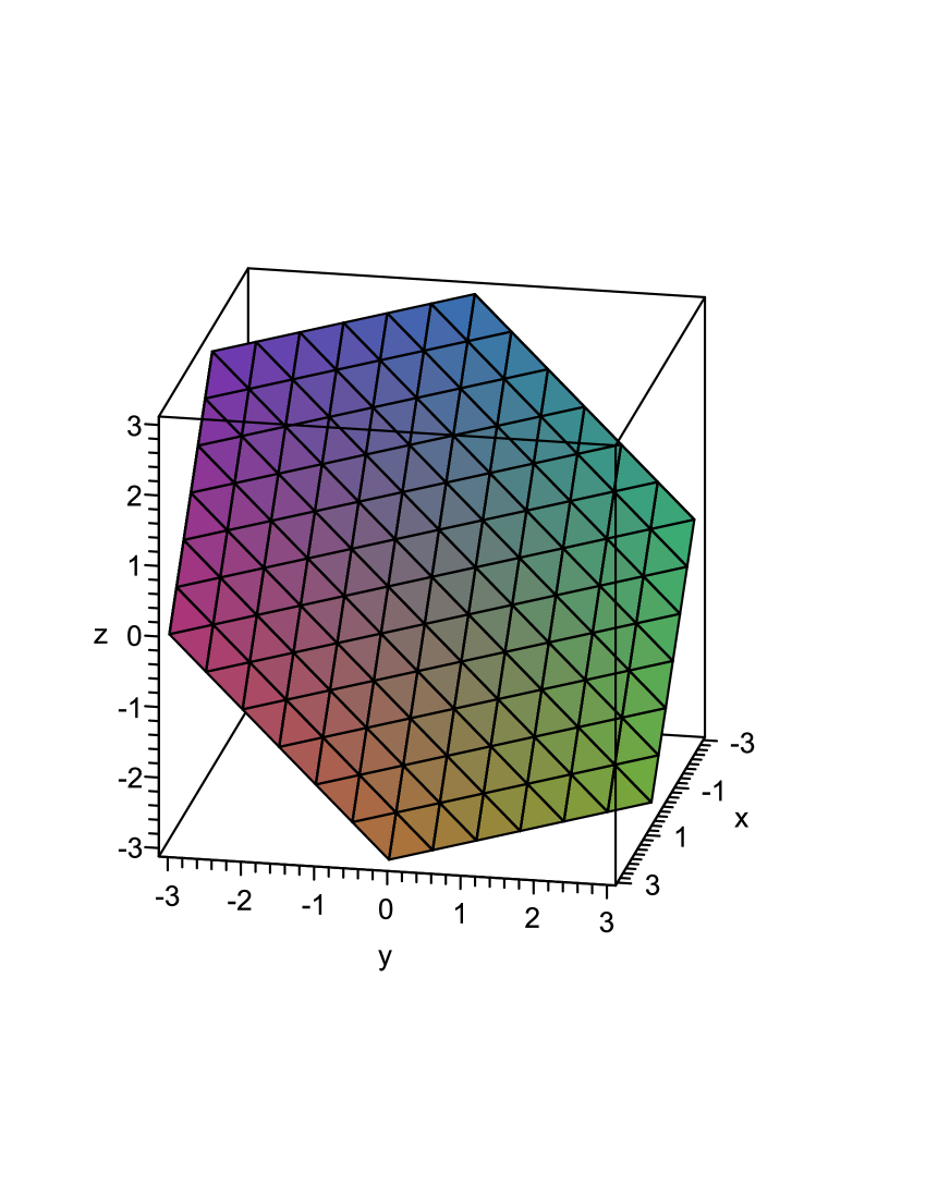
Figure 2: The graph of the $x+y+z=0$ plane.

In principle there are more possible generalization of the Ansatz available. One is the following:

$$u(x,y,z,t)=t^{-\alpha}f\left(\frac{\sqrt{x^{2}+y^{2}+z^{2}-a}}{t^{\beta}}\right):=t^{-\alpha}f(\omega)$$ (5)

which can be interpreted as an Euclidean vector norm or $L^{2}$ norm. Now we contract all the x coordinate of the velocity field $u$ (which are on a surface of a sphere with radius a) to a simple spatial coordinate. Unfortunately, if we consider the first and second spatial derivatives and plug them into the Navier-Stokes equation we cannot get a pure $\eta$ dependent ordinary differential equation(ODE) system some explicit $x,y,z$ or $t$ dependence tenaciously remain. For a telegraph-type heat conduction equation both these Ansatzes are useful to get solutions for the two dimensional case barna2 .

Now we concentrate on the first Ansatz (4) and search the solution of the Navier-Stokes PDE system in the following form:

$$u(x,y,z,t)=t^{-\alpha}f\left(\frac{x+y+z}{t^{\beta}}\right),\hskip 8.53581ptv(x,y,z,t)=t^{-\gamma}g\left(\frac{x+y+z}{t^{\delta}}\right),$$

$$w(x,y,z,t)=t^{-\epsilon}h\left(\frac{x+y+z}{t^{\zeta}}\right),\hskip 8.53581ptp(x,y,z,t)=t^{-\eta}l\left(\frac{x+y+z}{t^{\theta}}\right).$$ (6)

Where all the exponents $\alpha,\beta,\gamma,\delta,\epsilon,\zeta,\eta,\theta$ are real numbers. (Solutions with integer exponents are called self-similar solutions of the first kind, non-integer exponents mean self-similar solutions of the second kind.) The functions $f,g,h,l$ are arbitrary and will be evaluated later on. According to Eq. (2) we need to calculate all the first time derivatives of the velocity field, all the first and second spatial derivatives of the velocity fields and the first spatial derivatives of the pressure. All these derivatives are not presented in details. Note that both Eq. (2) and Eq. (8) have a large degree of exchange symmetry in the coordinates $x,y$ and $z$. Later we want to have an ODE system for all the four functions $f(\omega),g(\omega),h(\omega),l(\omega)$ which all have to have the same argument $\omega$. This dictates the constraint that $\beta=\delta=\zeta=\theta$ have to be the same real number which reduces the number of free parameters, (let’s use the $\beta$ from now on $\omega=\frac{x+y+z}{t^{\beta}})$. From this constrain follows that e.q. $u_{x}=\frac{f^{\prime}(\omega)}{t^{\alpha+\beta}}\approx v_{y}=\frac{f^{\prime}(\omega)}{t^{\gamma+\beta}}$ where prime means derivation with respect to $\omega$. This example shows the hidden symmetry of this construction which may helps us. For the better understanding we present the second equation of (2) after the substitution of the Ansatz (6).

$$-\alpha t^{-\alpha-1}f(\omega)-\beta t^{-\alpha-1}f^{\prime}(\omega)\omega+t^{-2\alpha-\beta}f(\omega)f^{\prime}(\omega)+t^{-\gamma-\alpha-\beta}g(\omega)f^{\prime}(\omega)+$$

$$t^{-\epsilon-\alpha-\beta}h(\omega)f^{\prime}(\omega)=\nu 3t^{-\alpha-2\beta}f^{\prime\prime}(\omega)-\frac{t^{-\mu-\beta}l^{\prime}(\omega)}{\rho}.$$ (7)

To have an ODE which only depends on $\omega$ (which is now the new variable instead of time t and the radial components) all the time dependences e.g. $t^{-\alpha-1}$ have to be zero OR all the exponents have to be the same. After some algebra it comes out that all the six exponents $\alpha-\zeta$ included for the velocity filed (the first three functions in Eq. (8)) have to be $+1/2$. The only exception is the term with the gradient of the pressure. There $\eta=1$ and $\theta=1/2$ have to be. Now in Eq. (9) each term is multiplied by $t^{-3/2}$. Self-similar exponents with the value of $+1/2$ are well-known from the regular Fourier heat conduction (or for the Fick’s diffusion) equation and gives back the fundamental solution which is the usual Gaussian function. For pressure the $\eta=1$ exponent means, a two times quicker decay rate of the magnitude than for the velocity field.

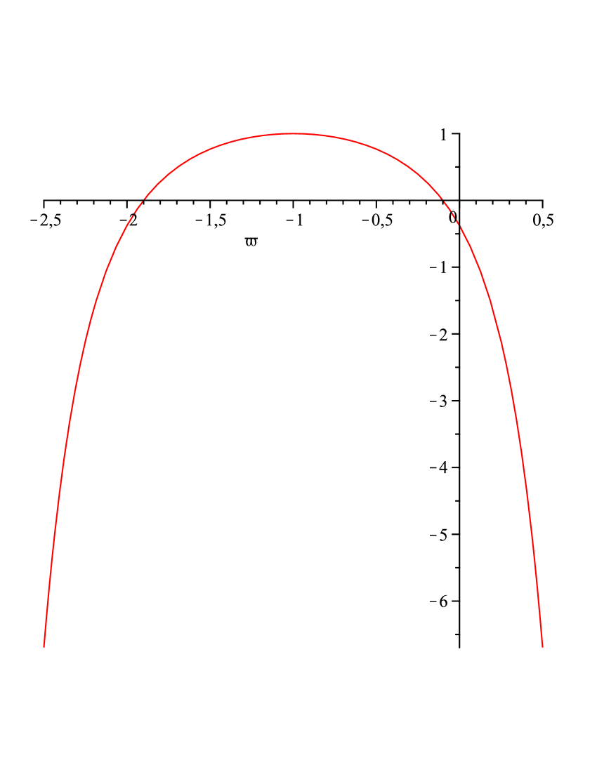
Figure 3: The $KummerM\left(-\frac{1}{4},\frac{1}{2},\frac{(\omega+c)^{2}}{6\nu}\right)$ function for $c=1$, and $\nu=0.1$.

Figure 4: The $KummerU\left(-\frac{1}{4},\frac{1}{2},\frac{(\omega+c)^{2}}{6\nu}\right)$ function for $c=1$, and $\nu=0.1$.

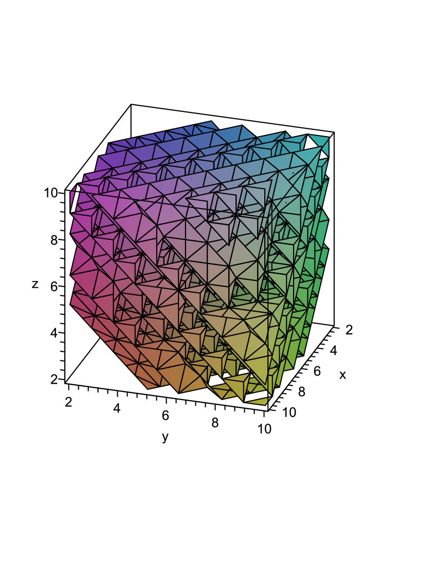
Figure 5: The implicit plot of the self-similar solution Eq. (17). Only the KummerU function is presented for $t=1,c_{1}=1,c_{2}=0,a=0,c=1$, and $\nu=0.1$.

Now we may write down the concrete form of the Ansatz (6)

$$u(x,y,z,t)=t^{-1/2}f\left(\frac{x+y+z}{t^{1/2}}\right)=t^{-1/2}f(\omega),\hskip 8.53581ptv(x,y,z,t)=t^{-1/2}g(\omega),$$

$$w(x,y,z,t)=t^{-1/2}h(\omega),\hskip 8.53581ptp(x,y,z,t)=t^{-1}l(\omega),$$ (8)

and the corresponding coupled ODE system

$$f^{\prime}(\omega)+g^{\prime}(\omega)+h^{\prime}(\omega) = 0$$

$$-\frac{1}{2}f(\omega)-\frac{1}{2}\omega f^{\prime}(\omega)+[f(\omega)+g(\omega)+h(\omega)]f^{\prime}(\omega) = 3\nu f^{\prime\prime}(\omega)-\frac{l^{\prime}(\omega)}{\rho}$$

$$-\frac{1}{2}g(\omega)-\frac{1}{2}\omega g^{\prime}(\omega)+[f(\omega)+g(\omega)+h(\omega)]g^{\prime}(\omega) = 3\nu g^{\prime\prime}(\omega)-\frac{l^{\prime}(\omega)}{\rho}$$

$$-\frac{1}{2}h(\omega)-\frac{1}{2}\omega h^{\prime}(\omega)+[f(\omega)+g(\omega)+h(\omega)]h^{\prime}(\omega) = 3\nu h^{\prime\prime}(\omega)-\frac{l^{\prime}(\omega)}{\rho}+a.$$ (9)

From the first (continuity) equation we automatically get

$$f(\omega)+g(\omega)+h(\omega)=c,\hskip 8.53581ptand\hskip 8.53581ptf^{\prime\prime}(\omega)+g^{\prime\prime}(\omega)+h^{\prime\prime}(\omega)=0$$ (10)

where c is proportional with the constant mass flow rate. Implicitly, larger c means larger velocities. From the second equation we can express $-\frac{l^{\prime}}{\rho}$ and can substitute it into the third and fourth equation. After some algebra we arrive at

$$\frac{f(\omega)-g(\omega)}{2}+\frac{\omega(f^{\prime}(\omega)-g^{\prime}(\omega))}{2}+3\nu(f^{\prime\prime}(\omega)-g^{\prime\prime}(\omega))$$

$$+[f(\omega)+g(\omega)+h(\omega)](g^{\prime}(\omega)-f^{\prime}(\omega))=0$$

$$\frac{f(\omega)-h(\omega)}{2}+\frac{\omega(f^{\prime}(\omega)-h^{\prime}(\omega))}{2}+3\nu(f^{\prime\prime}(\omega)-h^{\prime\prime}(\omega))$$

$$+[f(\omega)+g(\omega)+h(\omega)](h^{\prime}(\omega)-f^{\prime}(\omega))+a=0.$$

(11)

Now inserting $f^{\prime\prime}(\omega)=-g^{\prime\prime}(\omega)-h^{\prime\prime}(\omega)$, $f^{\prime}(\omega)=-g^{\prime}(\omega)-h^{\prime}(\omega)$ and $f(\omega)=c-g(\omega)-h(\omega)$ we get the final equation

$$9\nu f^{\prime\prime}(\omega)-3(\omega+c)f^{\prime}(\omega)+\frac{3}{2}f(\omega)-\frac{c}{2}+a=0.$$ (12)

The solutions are the Kummer functions abr

$$f(\omega)=c_{1}\cdot KummerU\left(-\frac{1}{4},\frac{1}{2},\frac{(\omega+c)^{2}}{6\nu}\right)+c_{2}\cdot KummerM\left(-\frac{1}{4},\frac{1}{2},\frac{(\omega+c)^{2}}{6\nu}\right)+\frac{c}{3}-\frac{2a}{3}$$ (13)

where $c_{1}$ and $c_{2}$ are integration constants. The KummerM function is defined by the following series

$$M(a,b,z)=1+\frac{az}{b}+\frac{(a)_{2}z^{2}}{(b)_{2}2!}+...+\frac{(a)_{n}z^{n}}{(b)_{n}n!}$$ (14)

where $(a)_{n}$ is the Pochhammer symbol

$$(a)_{n}=a(a+1)(a+2)...(a+n-1),(a)_{0}=1.$$ (15)

The KummerU function is defined from the KummerM function via the following form

$$U(a,b,z)=\frac{\pi}{sin(\pi b)}\left[\frac{M(a,b,z)}{\Gamma(1+a-b)\Gamma(b)}-z^{1-b}\frac{M(1+a-b,2-b,z)}{\Gamma(a)\Gamma(2-b)}\right]$$ (16)

where $\Gamma()$ is the Gamma function. Exhausted mathematical properties of the Kummer function can be found in abr .

Note, that the solution depends only on two parameters where the $\nu$ is the viscosity, and $c$ is proportional with the mass flow rate. Figure 3 and figure 4 show the KummerM and KummerU function for $c=1$ and $\nu=0.1$, respectively. For stability analysis we note that the power series which is applied to calculate the Kummer function has a pure convergence and a 30 digit accuracy was needed to plot the KummerU function, otherwise spurious oscillations occurred on the figure. Note, that for $\omega=6.5$ the KummerM goes to infinity, and $\omega\rightarrow\infty$ KummerU function goes to $\infty$ which is physically hard to understand, which means that the velocity field goes to infinity as well.

The complete self-similar solution of the x coordinate of the velocity reads

$$u(x,y,z,t)= t {}^{-1/2}f(\omega)=t^{-1/2}\left[c_{1}\cdot KummerU\left(\frac{-1}{4},\frac{1}{2},\frac{((x+y+z)/t^{1/2}+c)^{2}}{6\nu}\right)\right]+$$ (17)

$$t {}^{-1/2}\left[c_{2}\cdot KummerM\left(-\frac{1}{4},\frac{1}{2},\frac{((x+y+z)/t^{1/2}+c)^{2}}{6\nu}\right)+\frac{c}{3}-\frac{2a}{3}\right].$$

On figure 5 an implicit plot of Eq. (17) is visualized. The KummerU function was presented only, the used parameters are the following $c_{1}=1,c_{2}=0,t=1,c=1,\nu=0.1,a=0$. Note, that the initial flat surface of figure 2 is mapped into a complicated topological surface via the NS dynamical equation. The following phenomena happened, an implicit function is presented, we already mentioned that all the $x+y+z=0$ points considered to be the same. Therefore we got a multi-valued surface because for a fixed x numerical value various y+z combinations give the same argument inside the Kummer function. Unfortunately, this effect is hard to visualize. This can be understand as a kind of fingerprint of a turbulence-like phenomena which is still remained in the equation. An initial simple single-valued plane surface is mapped into a very complicated multivalued surface. Note, that for a larger value (now we presented KummerU() = 2 case) or for larger flow rate (c=1) the surface got even more structure. Therefore figure 5 presents only a principle. At this point we can also give statements about the stability of this solution, the solution the Kummer functions are fine, but for larger flow values a more precise and precise calculation of the solution surface is needed which means larger computational effort which is well known from the application of the NS equation.

From the integrated continuity equation $(f=c-g-f)$ we automatically get an implicit formula for the other two velocity components

$$v(x,y,z,t)+ w (x,y,z,t)=-t^{-1/2}\left[c_{1}\cdot KummerU\left(\frac{-1}{4},\frac{1}{2},\frac{((x+y+z)/t^{1/2}+c)^{2}}{6\nu}\right)\right]-$$ (18)

$$t {}^{-1/2}\left[c_{2}\cdot KummerM\left(-\frac{1}{4},\frac{1}{2},\frac{((x+y+z)/t^{1/2}+c)^{2}}{6\nu}\right)+\frac{c}{3}-\frac{2a}{3}\right]+c.$$

For explicit formulas of the remaining two velocity components the two ODEs of (11) have to be integrated. For $v(x,y,z,t)=t^{-1/2}g(\omega)$ the ODE is the following

$$-3\nu g^{\prime\prime}(\omega)+g^{\prime}(\omega)\left(-\frac{\omega}{2}+c\right)-\frac{g(\omega)}{2}+F(f^{\prime\prime}(\omega),f^{\prime}(\omega),f(\omega))=0$$ (19)

where $F(f^{\prime\prime}(\omega),f^{\prime}(\omega),f(\omega))$ contains the combination of the first and second derivatives of the Kummer functions. This is a second order linear ODE and the solution can be obtained with the following general quadrature

$$g(\omega)=\left[c_{2}+\int\left\{\frac{-c_{1}+\int F(f^{\prime\prime}(\omega),f^{\prime}(\omega),f(\omega))d\omega\cdot exp\left(\frac{-\omega^{2}/4+c\omega}{-3\nu}\right)}{3\nu}\right\}d\omega\right]exp\left(\frac{-\omega^{2}/4+c\omega}{3\nu}\right).$$ (20)

For the sake of simplicity we present the formulas of the first and second derivatives of the KummerU functions only

$$\frac{d}{d\omega}KummerU(a,b,\omega)=\frac{(\omega+a-b)KummerU(a,b,\omega)-KummerU(a-1,b,\omega)}{\omega}$$ (21)

and

$$\frac{d^{2}}{d\omega^{2}}KummerU(a,b,\omega)=\frac{1}{\omega^{2}}\left[a\left\{\omega aU(a+1,b,\omega)-\omega U(a+1,b,\omega)b+\omega U(a+1,b,\omega)\right.\right.$$

$$\left.\left.-aU(1+a,b,\omega)b+U(a,b,\omega)b+U(a+1,b,\omega)b^{2}-U(a+1,b,\omega)b\right\}\right].$$ (22)

Unfortunately, we could not find any closed form for $v(x,y,z,t)$ and for $w(x,y,z,t)$. Only $v$ the $x$ coordinate of the velocity ${\bf{v}}$ field can be evaluated in a closed form.

As we mentioned at the beginning there are analytic solutions available in the literature which are very similar to our one. Fushchich et al. fus present 19 different solutions for the full three dimensional NS and continuity equation. (For a better understanding we used the same notation here as well.) For the last (19th) solution they apply the following Ansatz of

$$u(z,t)=\frac{f(\omega)}{\sqrt{t}},\hskip 5.69054ptv(y,z)=\frac{g(\omega)}{\sqrt{t}}+\frac{y}{t},\hskip 5.69054ptw(z,t)=\frac{h(\omega)}{\sqrt{t}},\hskip 5.69054ptp(t,z)=\frac{l(\omega)}{\sqrt{t}}$$ (23)

where $\omega=z/{\sqrt{t}}$ is the invariant variable. The obtained ODE is very similar to ours (9)

$$h^{\prime}(\omega)+1 = 0$$

$$-\frac{1}{2}(f(\omega)+\omega f^{\prime}(\omega))+h(\omega)f^{\prime}(\omega) = f^{\prime\prime}(\omega),$$

$$\frac{1}{2}(g(\omega)+\omega g^{\prime}(\omega))+h(\omega)g^{\prime}(\omega) = g^{\prime\prime}(\omega),$$

$$-\frac{1}{2}(h(\omega)+\omega h^{\prime}(\omega))+h(\omega)h^{\prime}(\omega)+l^{\prime}(\omega) = f^{\prime\prime}(\omega).$$ (24)

The solutions are

$$f(\omega) = (\frac{3}{2}\omega-c)^{-1/2}exp\left[-\frac{1}{6}(\frac{3}{2}\omega-c)^{2}\right]w\left[-\frac{1}{12},\frac{1}{4},\frac{1}{3}(\frac{3}{2}\omega-c)^{2}\right]$$

$$g(\omega) = (\frac{3}{2}\omega-c)^{-1/2}exp\left[-\frac{1}{6}(\frac{3}{2}\omega-c)^{2}\right]w\left[-\frac{5}{12},\frac{1}{4},\frac{1}{3}(\frac{3}{2}\omega-c)^{2}\right]$$

$$h(\omega) = -\omega+c$$

$$l(\omega) = \frac{3}{2}c\omega-\omega^{2}+c_{1}$$ (25)

where $w$ is the Whitakker function, c and $c_{1}$ are integrational constants. Note that the Whitakker and the Kummer functions are strongly related to each other abr *

$$w(\kappa,\mu,z)=e^{-1/2z}z^{1/2+\mu}KummerM(1/2+\mu-\kappa,1+2\mu,z).$$ (26)

More details can be found in the original work fus .

As a second comparison we show the results of grassi . They also have a modified form of (2) which is the following

$$U_{1t}+cU_{1}+U_{2}U_{1y}+U_{3}U_{1z}-\nu(U_{1yy}+U_{1zz}) = 0,$$

$$U_{2t}+U_{2}U_{2y}+U_{3}U_{2z}+\pi_{y}-\nu(U_{2yy}+U_{2zz}) = 0,$$

$$U_{3t}+U_{2}U_{3y}+U_{3}U_{3z}+\pi_{z}-\nu(U_{3yy}+U_{3zz}) = 0,$$

$$U_{2y}+U_{3z}+c = 0$$ (27)

where $U_{i},i=1..3$ are the velocity components $U_{i}(y,z,t)$ and $\pi$ is the pressure, c stands for constants, $\nu$ is viscosity and additional subscripts mean derivations. After some transformation they get a linear PDA as follows

$$U_{1t}+k_{1}yU_{1y}+(\sigma-k_{1}z)U_{1z}-\nu(U_{1yy}+U_{1zz})=0$$ (28)

it is convenient to look the solution in the form of

$$U_{1}=Y(y)T(z)\Phi(t).$$ (29)

Note, that they also consider the full 3 dimensional problem, but the velocity filed has a restricted two dimensional(y,z) coordinate dependence. There are additional conditions but the general solution can be presented

$$\Phi = c_{1}exp(c_{2})t$$

$$Y = c_{3}M\left(-c_{4},\frac{1}{2},\frac{y^{2}}{2\nu}\right)+yc_{5}M\left(\frac{1}{2}-c_{4},\frac{3}{2},\frac{y^{2}}{2\nu}\right)$$

$$T \approx M\left(c_{6},\frac{1}{2},\frac{z^{2}}{2\nu}\right)+zM\left(\frac{1}{2}-c_{6},\frac{3}{2},\frac{z^{2}}{2\nu}\right)$$ (30)

where M is the Kummer M function as was presented below. The exact solution in grassi (4.10a-4.10c)* contains more constants as presented here. It is not our goal to reproduce the full calculation of grassi (which is not our work) we just want to give a guideline to their solution vigorously emphasising that our solution is very similar to the presented one. Note that in both results the arguments of the Kummer M function (13) and (30) are proportional to the square of the radial component divided by the viscosity, additionally one of the parameters is 1/2. As a last word we just would like to say, (as this example clearly shows) that the Lie algebra method is not the exhaustive method to find all the possible solutions of a PDA.

In summary: We introduced and gave a geometrical interpretation of a three-dimensional self-similar Ansatz. We applied it to the three-dimensional Navier-Stokes equation in Cartesian coordinates. The question of another Ansätze was mentioned briefly as well. Some part of the results could be written as Kummer functions. Unfortunately, some other parts of the results could not be written in closed forms. Further work is in progress, (we still have some hope) to learn something new from Eq. (19). We compared our results with other analytic solutions obtained from various Lie algebra studies. The structure of the result - the implicit coordinate dependence of the Kummer function - was analyzed as well. We hope that even this moderate result can give any simulating impetus to the investigation of the Navier-Stokes equation. Our solution can have some real interest and can be used as a test case for various numerical methods or commercial computer packages like Fluent or CFX.
The paper is dedicated to my first mathematics teacher ”Sanyi Bácsi”.

References

- (1) Y. Manwai, J. Math. Phys. 49 (2008) 113102.
- (2) V.N. Grebenev, M. Oberlack and A.N. Grishkov, Journ. of Nonlin. Mathem. Phys 15 (2008) 227.
- (3) W. I. Fushchich, W. M. Shtelen and S. L. Slavutsky J. Phys. A: Math. Gen. 24 (1990) 971.
- (4) V. Grassi, R.A. Leo, G. Soliani and P. Tempesta, Physica 286 (2000) 79 *, ibid 293 (2000) 421.
- (5) X.R. Hu, Z.Z. Dong, F. Huang et al., Z. Naturforschung A 65 (2010) 504.
- (6) S. N. Aristov and A. D. Polyanin, Russ. J. Math. Phys. 17 (2010) 1.
- (7) L. Sedov, Similarity and Dimensional Methods in Mechanics CRC Press 1993 * (Page 120).
- (8) H.Y Wu, J.X. Fei and C. L. Zheng, Commun. Theor. Phys. 54 (2010) 55.
- (9) C. Dai, Y. Wang and C. Yan, Optics Communications 283 (2010) 1489.
- (10) Y. Gau and S.Y. Lou, Commun. Theor. Phys. 52 (2009) 1031.
- (11) G.I. Baraneblatt, Similarity, Self-Similarity, and Intermediate Asymptotics Consultants Bureau, New York 1979.
- (12) Ya. B. Zel’dovich and Yu. P. Raizer Physics of Shock Waves and High Temperature Hydrodynamic Phenomena Academic Press, New York 1966.
- (13) J. Leray, Acta. Math. 63 (1934) 193.
- (14) J.R. Miller, M. O’Leray and M. Schonbeck, Math. Ann. 319 (2001) 809.
- (15) B.H. Gilding and R. Kersner, Travelling Waves in Nonlinear Diffusion-Convection Reactions, Progress in Nonlinear Differential Equations and Their Applications, Birkhäuser Verlag, Basel-Boston-Berlin, 2004, ISBN 3-7643-7071-8.
- (16) I.F. Barna and R. Kersner, J. Phys. A: Math. Theor. 43 (2010) 375210.
- (17) I.F. Barna and R. Kersner, Adv. Studies Theor. Phys. 5 (2011) 193.
- (18) M. Abramowitz and I. Stegun, Handbook of Mathematical Functions Dover Publication., Inc. New York. * Eq. 13.1.32.