Information filtering via preferential diffusion

Abstract

Recommender systems have shown great potential to address information overload problem, namely to help users in finding interesting and relevant objects within a huge information space. Some physical dynamics, including heat conduction process and mass or energy diffusion on networks, have recently found applications in personalized recommendation. Most of the previous studies focus overwhelmingly on recommendation accuracy as the only important factor, while overlook the significance of diversity and novelty which indeed provide the vitality of the system. In this paper, we propose a recommendation algorithm based on the preferential diffusion process on user-object bipartite network. Numerical analyses on two benchmark datasets, MovieLens and Netflix, indicate that our method outperforms the state-of-the-art methods. Specifically, it can not only provide more accurate recommendations, but also generate more diverse and novel recommendations by accurately recommending unpopular objects.

I Introduction.

The development of information technology brings great impact on human society. Therein, the most significant aspect is the revolutionary change in the ways of life. Twenty years ago, if one wants to buy something, he/she has to personally go to a physical shop and purchase, and then bring the things back home. It is impossible for him/her to compare the commodities in different markets located at different places in a short time. Now with the growth of the Internet and World Wide Web, we can almost manage our life at home. When we want to buy a book, we don’t need to go to bookstores any more to find it on bookshelves one by one, instead what we need to do is typing the title of this book on the website of Amazon — an online retailer of books. If we want to buy a cell phone, we can compare the prices on different web-shops at the same time without any transportation fee. Formerly, we usually go to a bar after working and enjoy making friends there, now we prefer online dating that allows us to reach people over the world. In a word, the Internet benefits us by providing a much more convenient way to get what we want. However, as a coin has two sides, Internet also brings us confusion — we face information overload. As we know, not all the online information are good or true or favorable by surfers. Therefore, we need to distinguish and select between valuable information and junks. In this sense, to get what we want or the most satisfied things becomes more and more difficult, since we face much more choices than before. A useful information filtering technology is search engine Brin1998 ; Kleinberg1999 , by which users can find the relevant information with properly chosen keywords or tags. However, search engines have two disadvantages which limit their applications. Firstly, they lack the consideration of personalization and thus return the same results to people no matter what their preferences are. Secondly, search engines require the users to know exactly what they want and extract some proper keywords to do the searching. However, sometimes the tastes or preferences can not be easily expressed by keywords or the users don’t even know what they want at all. In these cases, the search engines are of no avail.

To address these problems, recommender systems rise in response to the proper time and conditions, which form or work from a specific type of information filtering technique that attempts to recommend information items, such as movies, TV programs, videos, music, books, news, images and web pages, that are likely to be of interest to the users. The recommender systems don’t require specified keywords provided by users, instead they use the users’ historical activities and possible personal profiles to uncover their preferences or potential interests. Many recommendation algorithms have been developed, including collaborative filtering (CF) Goldberg1992 ; Schafer2007 ; Shang2009 , content-based analysis Pazzani2007 , spectral analysis Goldberg2001 ; Maslov2001 and iterative self-consistent refinement Laureti2006 ; Ren2008 . What most have in common is that they are based on similarity, either of users or objects or both. Such approach is under high risk of providing poor coverage of the space of relevant items. As a result, with recommendations based on similarity rather than difference, more and more users will be exposed to a narrowing band of popular objects. Although it seems more accurate to recommend popular objects than niche ones, being accurate is not enough McNee2006 . It was pointed out that the recommendations that are most accurate are sometimes not the recommendations that are useful to users. For example, would you use such a system that recommends the movies you indeed like but have seen before or just watched in the cinema? Diversity and novelty are also important criteria of algorithmic performance. A possible way to increase the recommendation diversity is utilizing the tags of objects Cattuto2007 ; ZhangZK ; ZhangZK2 . Another promising way is considering the dissimilar users’ contribution. It was shown that under the framework of collaborative filtering the dissimilar users can contribute to both accuracy and diversity of personalized recommendation Zeng2010 . However, these improvements are very limited.

Recently, some physical dynamics, including mass diffusion Zhou2007 ; Zhang2007b and heat conduction process Zhang2007a have been applied to design recommender systems. Zhou et al. proposed a network-based inference method (NBI) by considering the three-step mass diffusion starting from the target user on a user-object bipartite network Zhou2007 . This method has been demonstrated to be more accurate than the classical CF algorithm while with lower computational complexity. However, it has difficulty in generating diverse recommendations. The heat conduction process has been found its effectiveness in providing a diverse recommendation at the cost of accuracy. This diversity-accuracy dilemma can be effectively solved by coupling these two processes ZhouPNAS2010 . It was shown that not only does the hybrid algorithm outperform other methods but that, without relying on any semantic or context-specific information, it can be tuned to obtain significant gains in both accuracy and diversity of recommendations.

With the same motivation, we proposed an algorithm based on a preferential mass diffusion process on user-object bipartite networks, without consideration of heat conduction which may stealthily hurt accuracy. Numerical analyses on two benchmark datasets show that our method can give higher accurate as well as more diverse and novel recommendations than the hybrid algorithm, because of its high accurate recommendations on low-degree objects.

II Preferential diffusion method

A recommender system can be represented by a bipartite network $G(U,O,E)$, where $U=\{u_{1},u_{2},...,u_{m}\}$, $O=\{o_{1},o_{2},...,o_{n}\}$ and $E=\{e_{1},e_{2},...,e_{q}\}$ are the sets of users, objects and links respectively Shang2009 . Denote by $A_{m\times{n}}$ the adjacency matrix, where the element $a_{i\alpha}$ equals 1 if $u_{i}$ has collected object $o_{\alpha}$, and 0 otherwise.

The essential task of a recommender system is to generate a ranking list of the target user’s uncollected objects. The original diffusion-based recommendation algorithm, called network-based inference (NBI), was proposed in Ref. Zhou2007 . It was referred as ProbS algorithm in Ref. ZhouPNAS2010 . NBI works by assigning objects an initial level of resource denoted by the vector $\mathbf{f}$ (where $f_{\alpha}$ is the resource possessed by object $o_{\alpha}$), and then redistributing it via the transformation $\mathbf{f}^{\prime}=W\mathbf{f}$, where

$$w_{\alpha\beta}=\frac{1}{k_{o_{\beta}}}\sum_{l=1}^{m}\frac{a_{l\alpha}a_{l\beta}}{k_{u_{l}}},$$ (1)

is the resource transfer matrix, and $k_{o_{\beta}}=\sum_{i=1}^{n}a_{i\beta}$ and $k_{u_{l}}=\sum_{\gamma=1}^{m}a_{l\gamma}$ denote the degrees of object $o_{\beta}$ and user $u_{l}$ respectively. For a target user $u_{i}$, we assign one unit resource on those objects already collected by $u_{i}$ for simplicity, thus the initial resource vector $\mathbf{f}$ can be written as

$$f_{\alpha}=a_{i\alpha}.$$ (2)

That is to say, if object $o_{\alpha}$ is collected by user $u_{i}$ then it has one unit resource, otherwise 0. With this initial resource vector, the result of NBI is equivalent to a three-step random walk process starting from the target user on a bipartite network LiuWP2010 . Note that, if the initial resource vector is normalized by the target user’s degree, namely $f_{\alpha}=a_{i\alpha}/k_{ui}$, the results are exactly the same. In fact, the process of NBI is equivalent to resource-allocation which is also a random-work-based process. Given the initial resource distribution as shown in Eq. 2, the resource of each object will be redistributed according to Eq.1 where $w_{\alpha\beta}$ indicates how many proportion of resource that object $\alpha$ gives to object $\beta$. Then after the resource-allocation process, we obtain the final resource possessed by each object by summing up all the resources distributed from other objects. The recommendation list for user $u_{i}$ is generated by ranking all his/her uncollected objects in decreasing order according to their final resource.

A heterogenous initial resource distribution NBI algorithm (abbreviate as Heter-NBI) was proposed by Zhou et al. Zhou2008 , where the initial resource of object $o_{\alpha}$ is proportional to $k_{o_{\alpha}}^{\theta}$.Thus the initial resource vector of Heter-NBI can be written as $f_{\alpha}=a_{i\alpha}\cdot k_{o\alpha}^{\theta}$ where $\theta$ is a negative parameter. It was shown that Heter-NBI can give more accurate recommendations than the standard NBI. There are other two advanced recommendation algorithms. One is an improved algorithm by eliminating redundant correlations (called RE-NBI for short) ZhouNJP2009 , which is defined as

$$\mathbf{f}^{\prime}=(W+\eta{W^{2}})\mathbf{f},$$ (3)

where the elements of matrix $W$ are defined by Eq. 1, the initial resource vector $\mathbf{f}$ is defined by Eq. 2 and $\eta$ is a free parameter. This method has been approved to outperform some classical methods, such as the global ranking method, the cosine-similarity-based collaborative filtering Herlocker2004 , NBI and Heter-NBI for both accuracy and diversity by considering the high-order correlations between objects. The other method, referred as Hybrid-PH in this paper, is proposed in Ref. ZhouPNAS2010 , which is a hybrid algorithm combining the HeatS (i.e., heat conduction) and ProbS (i.e., mass diffusion) by incorporating the hybridization parameter $\lambda$ into the transition matrix normalization:

$$w_{\alpha\beta}=\frac{1}{k_{o_{\alpha}}^{1-\lambda}k_{o_{\beta}}^{\lambda}}\sum_{l=1}^{m}\frac{a_{l\alpha}a_{l\beta}}{k_{u_{l}}},$$ (4)

where $\lambda=0$ gives the pure HeatS algorithm, and $\lambda=1$ gives the ProbS (i.e., NBI).

Based on mass diffusion method and motivated by enhancing the algorithm’s ability to find unpopular and niche objects, we propose a preferential diffusion (PD) method for recommendation in user-object bipartite networks. The basic idea is that at the last step (i.e., diffusing from users to objects), the amount of resource that an object $o_{\alpha}$ received is proportional to $k_{o_{\alpha}}^{\varepsilon}$, where $\varepsilon\leq 0$ is a free parameter. In this case, the resource transfer matrix reads

$$w_{\alpha\beta}=\frac{1}{k_{o_{\beta}}\cdot{k_{o_{\alpha}}^{-\varepsilon}}}\sum_{l=1}^{m}\frac{a_{l\alpha}a_{l\beta}}{\mathcal{M}},$$ (5)

where $\mathcal{M}=\sum_{r=1}^{n}{a_{lr}k_{o_{r}}^{\varepsilon}}=k_{ul}\cdot\mathrm{E}(a_{lr}k_{o_{r}}^{\varepsilon})$. $\mathrm{E}(a_{lr}k_{o_{r}}^{\varepsilon})$ indicates the mean value of $k_{o_{r}}^{\varepsilon}$ over all the objects having been collected by user $u_{l}$. Here we consider the simplest initial resource vector defined by Eq. 2. Clearly, when $\varepsilon=0$ it will degenerate to NBI. Notice that, if we consider the NBI algorithm as a three step diffusion starting from target user to final objects (i.e., user$\rightarrow$object$\rightarrow$user$\rightarrow$object), then the Heter-NBI algorithm is essentially equivalent to the algorithm with preferential diffusion only at the first step, while PD considers the third step. However, their motivations are essentially different. Heter-NBI emphasizes that users who co-collected unpopular objects are more similar to each other than those co-collected popular objects. And thus the target user distributes more resource to his/her more similar users by giving more resource to their co-collected unpopular objects. However, after the third step diffusion the resource still can be centralized on some popular objects. The PD algorithm directly punishes the popular object by assigning more resource to the low-degree objects at the last step. Experimental results show that considering the preferential diffusion at the last step is much more effective than at the first step. In order to show that preferential diffusion at first step (i.e., Heter-NBI) and at last step (i.e., PD) play different roles in recommendation, we further investigate the PD algorithm with heterogenous initial resource distribution, called Heter-PD, which is controlled by two tunable parameters. Comparing with all the mentioned algorithms in this paper, Heter-PD performs the best over all five evaluation metrics considered in this paper (see section 3 for the definitions of evaluation metrics). Comparing Eq. 4 with Eq. 5, we can find that if we assume that for user $u_{l}$ who has collected object $o_{\beta}$, the approximation $\mathrm{E}(a_{lr}k_{o_{r}}^{\varepsilon})\approx k_{o_{\beta}}^{\varepsilon}$ holds, namely the mean value of $k_{o_{r}}^{\varepsilon}$ over all the objects having collected by user $u_{l}$ always equals $k_{o_{\beta}}^{\varepsilon}$, PD is equivalent to the hybrid algorithm by setting $\varepsilon=\lambda-1$. However, this assumption is too strong to be satisfied in reality.

Note that, we didn’t consider the preferential diffusion at the second step from the object side to the user side (PD-II for short). The main reason is that this method may lead to some illogical results. Considering the case that the target user $u_{i}$ selected a very popular object $o_{\alpha}$ which is also selected by another user $u_{j}$ who is assumed to be a new user of the system and only selected $o_{\alpha}$. Via the PD-II method, $u_{j}$ will obtain more resource from $o_{\alpha}$ than other users who also selected $o_{\alpha}$, leading to the conclusion that $u_{j}$ is more similar to $u_{i}$. Apparently this result is wrong, since a new user usually selects popular objects, which is a common behavior in such kind of systems Shang2010 , and it is unreasonable to say this new user is more similar to the target user just according to such a common behavior. In addition, we have tested the performance of PD-II method. Comparing with standard NBI method, the improvement of accuracy (measured by ranking score) is very slight around 1% on MovieLens data and 0.6% on Netflix data. Therefore, we didn’t consider this method for further analysis.

III Data and metrics

To test the algorithmic performance, we use two benchmark datasets. The MovieLens (http://www.grouplens.org/) data consists of 1682 movies (objects) and 943 users who can vote for movies with five level ratings from 1 (i.e., worst) to 5 (i.e., best). The original data contains $10^{5}$ ratings. Here we only consider the ratings higher than 2. After coarse gaining the data contains 82520 user-object pairs. The Netflix data (http://www.netflixprize.com/) is a random sampling of the whole records of user activities in Netflix.com. It consists of 10000 users, 6000 movies and 824802 links. Similar to the MovieLens data, only the links with ratings no less than 3 are considered. After data filtering, there are 701947 links left. To test the algorithmic performance, the data (i.e., known links) is randomly divided into two parts: The training set $E^{T}$ contains 90% of the data, and the remaining 10% of data constitutes the probe set $E^{P}$. Notice that, any isolate object can not be recommended to users through the algorithms considered in this paper. Therefore to ensure the connectivity of the whole network, each time before moving a link to the probe set, we first check if this removal will result in isolate user or object, and we do not allow the removal that leads to unconnected nodes.

Accuracy is the most important aspect to evaluate the recommendation algorithmic performance. A good algorithm is expected to give accurate recommendations, namely higher ability to find what the users like. Here we use Ranking Score Zhou2007 to measure the ability of a recommendation algorithm to produce a good ordering of objects that matches the user’s preference. For a target user, the recommender system will return a ranking list of all his uncollected object to him. For each hidden user-object relation (i.e., the link in probe set), we measure the rank of this object in the recommendation list of this user. For example, if there are 1000 uncollected objects for user $u_{i}$, and object $o_{\alpha}$ is at 10th place, we say the position of this object is 10/1000, denoted by $RS_{i\alpha}=0.01$. A good algorithm is expected to give high ranks to the hidden objects, and thus leading to small $RS$. Averaging over all the hidden user-object relations, we obtain the mean value of ranking score $RS$ that can be used to evaluate the algorithm’s accuracy, namely

$$RS=\frac{1}{|E^{P}|}\sum_{i\alpha\in E^{P}}RS_{i\alpha},$$ (6)

where $i\alpha$ denotes the probe link connecting $u_{i}$ and $o_{\alpha}$. Clearly, the smaller the ranking score, the higher the algorithm’s accuracy, and vice versa. Since real users usually consider only the top part of the recommendation list, a more practical measure may be to consider the number of user’s hidden links contained in the top-$L$ places. Therefore, we adopt another accuracy metric called Precision. For a target user $u_{i}$, the precision of recommendation, $P_{i}(L)$, is defined as

$$P_{i}(L)=\frac{d_{i}(L)}{L},$$ (7)

where $d_{i}(L)$ indicates the number of relevant objects (namely the objects collected by $u_{i}$ in the probe set) in the top-$L$ places of recommendation list. Averaging the individual precisions over all users with at least one hidden link, we obtain the mean precision $P(L)$ of the whole system.

Besides accuracy, diversity is taken into account as another important aspect to evaluate the recommendation algorithm. There are two kinds of diversity. One is called Inter-Diversity which considers the uniqueness of different users’ recommendation lists. Given two users $u_{i}$ and $u_{j}$, the difference between their recommendation lists can be measured by the Hamming distance Zhou2008 ,

$$H_{ij}(L)=1-\frac{C_{ij}(L)}{L},$$ (8)

where $C_{ij}(L)$ is the number of common objects in the top-$L$ places of both lists. Clearly, if $u_{i}$ and $u_{j}$ have the same list, $H_{ij}(L)=0$, while if their lists are completely different, $H_{ij}(L)=1$. Averaging $H_{ij}(L)$ over all pairs of users we obtain the mean distance $H(L)$, for which greater or lesser values mean, respectively, greater or lesser personalization of users’ recommendation lists. A good algorithm should not only give diverse recommendations among users (i.e., high inter-diversity), but also provide diverse recommendations for a single user (i.e., high intra-diversity) ZhouNJP2009 ; Ziegler2005 . The latter can be measured by Intra-Similarity. For a target user $u_{i}$, his recommended objects are {$o_{1},o_{2},\cdots,o_{L}$}, then the intra-similarity of $u_{i}$’s recommendation list is defined as ZhouNJP2009 :

$$I_{i}(L)=\frac{1}{L(L-1)}\sum_{\alpha\neq\beta}s^{o}_{\alpha\beta},$$ (9)

where $s^{o}_{\alpha\beta}$ is the similarity between objects $o_{\alpha}$ and $o_{\beta}$ in $u_{i}$’s recommendation list. There are many similarity indices that can be used to quantify the similarity between objects Zhou2009 . Here we adopt the widely used cosine similarity to measure object similarity. For two objects $o_{\alpha}$ and $o_{\beta}$ their similarity is defined as

$$s^{o}_{\alpha\beta}=\frac{1}{\sqrt{k_{o_{\alpha}}k_{o_{\beta}}}}\sum_{l=1}^{m}a_{l\alpha}a_{l\beta}.$$ (10)

Averaging $I_{i}(L)$ over all users we obtain the mean intra-similarity $I(L)$ for the system. A good recommendation algorithm is expected to give fruitful recommendations and has the ability to guide or help the users to exploit their potential interest fields, and thus leads to a lower intra-similarity (i.e., higher intra-diversity).

High accurate recommendations might not be satisfied by the users. For example, recommending popular film Avatar to a user on MovieLens website is not always the best, because he/she might have already seen this film at the cinema. A diverse recommender system is expected to find the niche or unpopular objects that can not be easily known by other ways yet match users’ preferences. The metric Popularity quantifies the capacity of an algorithm to generate novel and unexpected results, that is to say, to recommend less popular items unlikely to be already known about. The simplest way to calculate popularity is to use the average collected times over all the recommended items, as:

$$N_{i}(L)=\frac{1}{L}\sum_{o_{\alpha}\in O_{R}^{i}}{k_{o_{\alpha}}},$$ (11)

where $O_{R}^{i}$ is the recommendation list for user $u_{i}$. Clearly, lower popularity indicates higher novelty and surprisal. Averaging $N_{i}(L)$ over all users we obtain the mean popularity $N(L)$ for the system.

Table 1: Algorithmic performance for MovieLens data. The precision, intra-similarity, hamming distance and popularity are corresponding to $L=50$. Heter-NBI is an abbreviation of NBI with heterogenous initial resource distribution, proposed in Ref. Zhou2008 . RE-NBI is an abbreviation of redundant-eliminated NBI, proposed in Ref. ZhouNJP2009 . Hybrid-PH refers to the hybrid method which combines ProbS and HeatS algorithms. PD is an abbreviation of preferential diffusion method presented in this paper. Heter-PD is an abbreviation of PD with heterogenous initial resource distribution. The parameters (ranging in the interval [0,1] for Hybrid-PH and [-1,0] for the rest five algorithms with step 0.05) for the parameter-dependent algorithms are set as the ones corresponding to the lowest ranking scores (for Heter-NBI, $\theta_{\texttt{opt}}=-0.80$; for RE-NBI, $\eta_{\texttt{opt}}=-0.75$; for Hybrid-PH, $\lambda_{\texttt{opt}}=0.20$; for PD, $\varepsilon_{\texttt{opt}}=-0.85$; for Heter-PD, $(\theta,\varepsilon)_{\texttt{opt}}=(-0.25,-0.8)$). Each number is obtained by averaging over five runs with independently random division of training set and probe set. The entries corresponding to the best performance over all methods (except Heter-PD) are emphasized in black.

Algorithms	Ranking Score	Precision	Intra-Similarity	Hamming Distance	Popularity
NBI	0.106	0.071	0.355	0.617	233
Heter-NBI	0.101	0.074	0.340	0.680	220
RE-NBI	0.082	0.085	0.326	0.788	189
Hybrid-PH	0.085	0.083	0.296	0.821	167
PD	0.082	0.084	0.282	0.847	155
Heter-PD	0.081	0.086	0.278	0.858	153

Table 2: Algorithmic performance for Netflix data. The precision, intra-similarity, hamming distance and popularity are corresponding to $L=50$. The parameters (ranging in the interval [0,1] for Hybrid-PH and [-1,0] for the rest five algorithms with step 0.05) for the parameter-dependent algorithms are set as the ones corresponding to the lowest ranking scores (for Heter-NBI, $\theta_{\texttt{opt}}=-0.70$; for RE-NBI, $\eta_{\texttt{opt}}=-0.75$; for Hybrid-PH, $\lambda_{\texttt{opt}}=0.20$; for PD, $\varepsilon_{\texttt{opt}}=-0.85$; for Heter-PD, $(\theta,\varepsilon)_{\texttt{opt}}=(-0.2,-0.8)$). Each number is obtained by averaging over five runs with independently random division of training set and probe set. The entries corresponding to the best performance over all methods (except Heter-PD) are emphasized in black.

Algorithms	Ranking Score	Precision	Intra-Similarity	Hamming Distance	Popularity
NBI	0.050	0.050	0.366	0.424	2366
Heter-NBI	0.047	0.051	0.341	0.545	2197
RE-NBI	0.039	0.062	0.336	0.629	2063
Hybrid-PH	0.045	0.057	0.311	0.625	1998
PD	0.041	0.057	0.295	0.639	1900
Heter-PD	0.040	0.057	0.266	0.708	1742

Figure 1: The ranking score $RS$ vs. $\varepsilon$. Each data point is obtained by averaging over five runs, each of which has an independently random division of training set and probe set. The optimal parameters $\varepsilon$ for MovieLens and Netflix, corresponding to the minimal $RS$, both equal to -0.85.

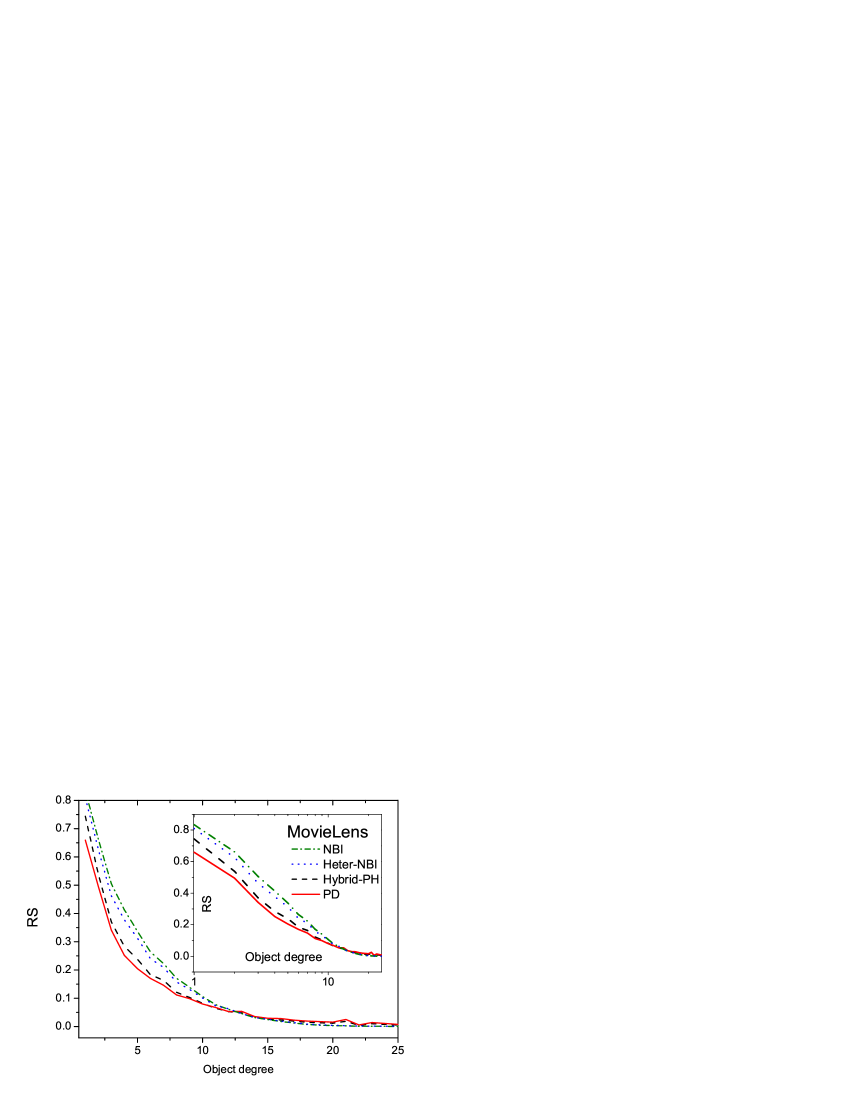
Figure 2: (Color online) The dependence of ranking score $\langle RS\rangle$ on the object degree. For a given $x$, its corresponding RS is obtained by averaging over all the objects whose degrees are in the range of ($a(x^{2}-x)$,$a(x^{2}+x)$], where $a$ is chosen as $\frac{1}{2}\log 5$ for a better illustration. Insets show RS against logarithm of $x$.

Figure 3: (Color online) The dependence of precision on parameter $\varepsilon$. Each data point is obtained by averaging over five independent runs with data division identical to the case shown in figure 1. The vertical dotted line indicates the optimal parameter $\varepsilon$ subject to the lowest ranking score.

IV Results

Summaries of the results for all algorithms and metrics on MovieLens and Netflix datasets are shown respectively in Table 1 and Table 2. The so-called optimal parameters are subject to the lowest ranking score. And the other four metrics, namely precision, intra-similarity, hamming distance and popularity, are obtained at the optimal parameters. Clearly, PD outperforms Heter-NBI over all the five evaluation metrics. Among all four previous algorithms, Re-NBI gives the highest accuracy by considering the high-order correlations between objects, while Hybrid-PH has the best performance on diversity and novelty. Comparing with these two outstanding algorithms, PD can reach or closely near the best accuracy without considering high-order correlation between objects, and provide much more diverse results. By considering the heterogenous initial resource distribution the algorithmic performance can be further improved. For example, in MovieLens Heter-PD decreases the ranking score to 0.081 with the parameters $\theta=-0.25$ and $\varepsilon=-0.8$, which is the lowest among all the methods referred in this paper. Although with a heterogenous initial resource distribution, both accuracy and diversity can be improved, comparing with pure PD algorithm, such improvements are less remarkable. This indicates that PD actually plays the main role of improvements.

For PD algorithm, the dependence of parameter $\varepsilon$ on accuracy measured by ranking score is shown in figure 1. The optimal values of parameter $\varepsilon$ corresponding to the lowest ranking score on two datasets are both equal to 0.85. Comparing with the standard case NBI, namely $\varepsilon=0$, the ranking score can be reduced by 23% for MovieLens and 18% for Netflix. We further investigate the dependence of ranking score (RS) on the object degree of four methods, namely NBI, Heter-NBI, Hybrid-PH and our method PD. The results are shown in figure 2. Notice that, for a given $x$, its corresponding RS is obtained by averaging over all the objects whose degrees are in the range of ($\frac{x^{2}-x}{2}\log 5$,$\frac{x^{2}+x}{2}\log 5$]. Insets show the RS against logarithm of $x$. It can be seen that the ranking score decreases with the increasing of the object degree for all these four algorithms. This indicates that in average popular objects can be more accurately recommended than the unpopular objects. The significant differences of these four algorithms are embodied on their ability of accurately recommending unpopular objects. Clearly, PD works best for this task, and is followed by Hybrid-PH. Moreover, comparing the results of Heter-NBI with PD, we can see that although they both consider the preferential diffusion from user to object, considering at the first step (i.e., Heter-NBI) has much less effect on the unpopular objects than directly acting on the final step (i.e., PD).

Figure 3 shows how the precision changes with the parameter $\varepsilon$ for four typical lengths of recommendation list. Given $L$ there exists an optimal parameter $\varepsilon$ leading to the highest precision. Although this optimal parameter $\varepsilon_{1}$ is different from that subject to the lowest ranking score $\varepsilon_{2}$, the precision obtained with $\varepsilon_{2}$ is also considerably higher than that obtained by NBI. For example, when $L=50$ with the optimal parameter corresponding to the lowest ranking score, the precision is prominently improved by 18% and 14% for MovieLens and Netflix respectively.

Hamming distance actually measures the ability that an algorithm give personalized recommendation. How the parameter $\varepsilon$ affects the Hamming distance is shown in figure 4. Clearly, a smaller $\varepsilon$ leads to a higher Hamming distance (i.e., higher inter-diversity), and thus a more personalized recommendation. Comparing with the standard case NBI, given $L=50$, Hamming distance can be enhanced by 37% for MovieLens and 56% for Netflix with optimal parameters corresponding to their respective lowest ranking scores, even higher than the Hybrid-PH algorithm. As a result, our method has higher ability to find the niche (unpopular) objects that may be liked by users, and thus give a more personalized recommendation to the target user. To give more evidences, for a given algorithm we collect the top-$L$ recommended objects for each user. Denote by $d$ the number of distinct objects among all the recommended objects. Then we rank the $d$ objects according to their recommended times, denoting by $Q_{i}$ ($i=1$, $\cdots$, $d$), in decreasing order. The relationships between the objects’ recommended times $Q$ and their ranks are shown in figure 5. We have tested for many different $L$, and here take $L=50$ and $L=100$ as typical examples. Two important phenomena can be obtained from figure 5. Firstly, comparing three algorithms, NBI, Hybrid-PH with $\lambda=0.2$ and PD with $\varepsilon=-0.85$, we have $d_{PD}>d_{Hybrid}>d_{NBI}$. That is to say PD provides larger number of distinct objects to users than NBI and Hybrid-PH. For example, when the length of recommendation list is 50, in MovieLens data, NBI can only recommend 293 distinct objects, Hybrid-PH can recommend 787 distinct objects, while PD increases this number to more than 1000. In Netflix data, for the case $L=50$, more than 5000 distinct objects can be recommended through PD algorithm, namely almost every object has the chance to be recommended. Secondly, the curves for NBI are remarkably steeper than these from Hybrid-PH and PD. Take the MovieLens data for example (the case $L=50$), with NBI algorithm, six movies are recommended over six hundred times. Since there are only 943 users in this dataset, it means that each of these movies is recommended to more than two-thirds of the users. The result with Hybrid-PH is much better, the No.1 object is recommended 341 times. However, comparing with Hybrid-PH, see the insets of figure 5, PD performs better, which indicates that with PD algorithm users are more likely to be recommended with different objects, namely PD can provide more personalized recommendations.

Figure 4: (Color online) The Hamming distance vs. $\varepsilon$. Each data point is obtained by averaging over five independent runs with data division identical to the case shown in figure 1. The vertical dotted line indicates the optimal parameter $\varepsilon$ subject to the lowest ranking score.

Figure 5: (Color online) The relationship between the recommended times $Q$ of objects and their ranks for two datasets. Insets of two MovieLens sub-figures show the results of top-200 frequently recommended objects. Insets of two Netflix sub-figures show $Q$ against logarithm of $x$ (i.e., Rank). For NBI, only the objects inside the blue region have the chance to be recommended.

Another metric to measure the algorithm’s diversity is intra-similarity. Different from Hamming distance, intra-similarity measures the ability that an algorithm provides diverse recommendations for a single user. The dependence of intra-similarity on parameter $\varepsilon$ is shown in figure 6. It shows that the parameter $\varepsilon$ is positively correlated with intra-similarity, namely the smaller $\varepsilon$ the lower intra-similarity (i.e., higher intra-diversity). Comparing with NBI, when $L=50$, intra-similarity can be decreased by 21% for MovieLens and 23% for Netflix with optimal parameters corresponding to their respective lowest ranking scores. Even comparing with the Hybrid-PH algorithm, the improvement can reach up to 5% for both datasets. This claims that our method is effective to generate more fruitful recommendations. Furthermore, we investigate how the two parameters ($\varepsilon$, $L$) affect intra-similarity. The intra-similarity $I$ in ($\varepsilon$, $L$) plane for two datasets are shown in figure 7. The dashed line indicates the intra-similarity of the system which is obtained by averaging $s_{\alpha\beta}^{o}$ over all the object pairs. Thus the intra-similarity as obtained from ($\varepsilon$, $L$) on the dashed line is equal to that of $L$ randomly chosen objects from the system. The left region has lower intra-similarity while the right region has higher intra-similarity. As a metaphor, one can think the dashed line as a plane lens keeping the same size of the user’s vision. And in the left region especially the area corresponding to smaller $\varepsilon$ and larger $L$, the algorithm is like a concave lens that broadens the user’s vision, while in the right region corresponding to larger $\varepsilon$ and smaller $L$, the algorithm is like a convex lens that narrows user’s vision. The focal length is determined by parameter $\varepsilon$. A smaller $\varepsilon$ in the left region indicates a smaller focal length for concave lens, and hence a broader view, while in the right region indicates a larger focal length for convex lens, hence a narrow view.

In figure 8, we report the dependence of popularity on parameter $\varepsilon$. Similar with intra-similarity, a smaller $\varepsilon$ yields a smaller popularity $P$, and thus a more novel recommendation. Comparing with the NBI, popularity can be remarkably improved by 33% and 23% for MovieLens and Netflix datasets. Even comparing with the Hybrid-PH algorithm, the improvement can reach 7% and 5% respectively.

Figure 6: (Color online) The intra-similarity as a function of $\varepsilon$. Each data point is obtained by averaging over five independent runs with data division identical to the case shown in figure 1. The vertical dotted line indicates the optimal parameter $\varepsilon$ subject to the lowest ranking score.

Figure 7: (Color online) The intra-similarity $I$ in ($\varepsilon$, $L$) plane for two datastes. The numerical simulation run over the parameter $L$ in the interval [10,100] with step length equal to 10, and the parameter $\varepsilon$ in the interval [-1,0] and [-1.2,0] for MovieLens and Netflix respectively, with step 0.05. All the results are obtained by averaging over five independent runs with data division identical to the case shown in figure 1. The dashed line indicates that with the parameter combination ($\varepsilon$, $L$) on this line the intra-similarity equals the value of the system.

Figure 8: (Color online) The dependence of popularity (i.e., average degree) on $\varepsilon$. Each data point is obtained by averaging over five independent runs with data division identical to the case shown in figure 1. The vertical dotted line indicates the optimal parameter $\varepsilon$ subject to the lowest ranking score.

V Effects of data sparsity

In this section, we investigate the effects of data sparsity on the algorithmic performance. Since Hybrid-PH is the most similar algorithm with our method, we choose it for comparison (although RE-NBI is more accurate, it considers the high-order correlations between objects). We investigate the effects of data sparsity on the algorithmic performance in two ways: (i) For the whole dataset, we select $p$% (ranging from 10% to 90% with step 10%) links as training set, and the rest $(100-p)$% links constitute the probe set. Clearly, lower $p$ indicates sparser data (i.e., less information). (ii) Given a 90%-10% division of training set and probe set, we randomly choose $p$% of the known links in the prepared training set to predict the links in probe set. To do this, the probe links keep unchanged. For example, $p=$10 means that we actually use 9% of the whole dataset to predict the links in probe set which contains 10% links of the whole dataset. Lower $p$ indicates sparser data. The numerical results on two datasets are shown in figure 9 for method (i) and figure 10 for method (ii). Each point is obtained with the optimal parameter subject to the lowest ranking score. From figure 9, it can be seen that the ranking score decreases with the increasing of the size of the training set, which agrees with the intuition that we can obtain better recommendation with more information. Furthermore the optimal parameters of both methods decrease with the increasing of $p$ for both methods. It shows that when training set contains 10% links, the optimal parameters are $\lambda=1$ for Hybrid-PH and $\varepsilon=0$ for PD, which are all corresponding to the standard case NBI. Insets show the RS-improvement of PD comparing with Hybrid-PH, which is defined as

$$Improvement=\frac{RS_{Hybrid}^{*}-RS_{PD}^{*}}{RS_{Hybrid}^{*}},$$ (12)

where $RS^{*}$ indicates the lowest ranking score for a given training and probe set division. Generally speaking, the RS-improvement increases with the increasing of the size of training set. That is to say, PD performs much better than Hybrid-PH for denser datasets. The qualitative behaviors in figure 10 are the same as what we obtained in figure 9, which further demonstrates that PD can give much better predictions than Hybrid-PH for denser datasets.

Figure 9: (Color online) The ranking score changes with the size of training set measured by the percentage of the whole data set. That is to say, we change the size of training set from 10% to 90% to respectively predict the rest 90% to 10%. Each data point is obtained with the parameter ($\varepsilon\in[-1,0]$ for PD and $\lambda\in[0,1]$ for Hybrid-PH with step 0.05) subject to the lowest RS. The optimal parameters are labelled in black for PD and red for Hybrid-PH. Insets show the RS-improvement of PD comparing with Hybrid-PH against the size of training set.

Figure 10: (Color online) The ranking score changes with the size of training set measured by the percentage of the 90% training set. That is to say, given a 90%-10% division of training set and probe set, we randomly choose $p$% of the known links in training set to predict the links in the unchanged probe set. Each data point is obtained with the parameter ($\varepsilon\in[-1,0]$ for PD and $\lambda\in[0,1]$ for Hybrid-PH with step 0.05) subject to the lowest RS. The optimal parameters are labelled in black for PD and red for Hybrid-PH. Insets show the RS-improvement of PD comparing with Hybrid-PH against the size of training set.

VI Conclusion and Discussion

The preferential diffusion proposed in this paper is a kind of biased random walk taking into account the heterogeneity of users’ degrees. The present process indeed defines a new local index of similarity in bipartite networks (like the original NBI algorithm is corresponding to the so-called resource-allocation similarity index Zhou2009 ; Lu2009 ) and thus it has potential applications in similarity-based link prediction Liben-Nowell2007 ; Lu2011 , community detection Pan2010 , node classification ZhangQM2010 , and so on. The biased random walk itself has already found extensive application in many branches of science and engineering, including detecting the navigation rules on complex network Fronczak2009 , quantifying the centrality of vertex and edge Lee2009 , modeling the animal movements Codling2010 and information discovery in wireless sensor networks Rachuri2009 . Here we applied the biased random walk in dealing with the information filtering process, which may also broaden the understanding of the applicability of biased random walk

Accuracy metrics have been widely used to evaluate the performance of recommendation algorithms and considered to be the most important factor. For example, the Netflix Prize Bennett2007 focuses only on accuracy. However, user satisfaction is not always correlated with high recommendation accuracy Ziegler2005 ; McNee2002 . The recommendations on popular objects (those are more easily to be found in other channels) are less likely to excite users. On the contrary, the unexpected and fortuitous recommendations which are usually related with cold objects are more favorable. Such serendipity recommendation will improve user experience and thus enhance their loyalty to the system. In order to provide accurate as well as diverse and novel recommendations, in this paper, motivated by the perspective of physics, we proposed an algorithm, named PD, based on preferential diffusion process on bipartite networks. We tested our algorithm on two benchmark datasets, MovieLens and Netflix, and applied five metrics, from the aspects of accuracy, diversity and novelty, to evaluate the algorithmic performance. Comparing with the standard algorithm NBI, the accuracy measured by ranking score can be further improved by 23% for MovieLens and 18% for Netflix. Even comparing with the state-of-the-art algorithm, Hybrid-PH, the improvement can reach 4% for MovieLens and 9% for Netflix. Moreover, the performance of PD can be further improved by considering a heterogenous initial resource configuration.

Furthermore, statistical result on the ranking score of individual objects shows that our method has much higher ability to accurately recommend the low-degree objects. That is to say, such prominent improvement on accuracy comes mainly from the highly accurate recommendation on unpopular objects, and thus it indeed enhances the recommendation diversity and novelty. For example, if we recommend 50 objects to each user, in MovieLens, NBI can only recommend 293 distinct objects to all users, Hybrid-PH can recommend 787 distinct objects, while PD increases this number to more than 1000. In Netflix data, more than 5000 distinct objects can be recommended through PD algorithm, namely almost every object has the chance to be recommended. Specially, we found that the recommender system may play different roles from the aspect of intra-similarity — the similarity within a user’s recommendation list, which is determined by the algorithm’s parameter $\varepsilon$ and the length of recommendation list $L$. Given ($\varepsilon$, $L$), if the intra-similarity generated by algorithm is higher than that of $L$ randomly selected objects (i.e., average intra-similarity of the whole system), the recommender system plays the role as a convex that narrows users’ vision, whereas if intra-similarity generated by algorithm is lower than that of the system, the recommender system plays the role as a concave that broadens users’ vision. Besides, we investigated the dependence of algorithm performance on data density. The results show that comparing with Hybrid-PH, PD algorithm gives more significant improvement for denser data.

A good recommendation algorithm can guide the system for a better development. You can think that the system itself and the recommendation algorithm constitute a symbiotic system. Generally speaking, there is no best recommendation algorithm, but the most suitable algorithm for a given system or a user. Just like the marriage game Omero1997 : choose the right but not the best. In this sense, the most equitable evaluation on recommendation algorithm should be based on the user experience which is difficult to capture in metric. Notice that, the optimal algorithm (or parameter) for the whole system is usually different from the optimal algorithm (or parameter) for an individual user. Thus an applicable and feasible way is building an open recommender system where users can help themselves to find their best experienced algorithm (or parameter). For example, we can set a bar controlling the parameter of the algorithm on the website. Take the PD algorithm as an example, the user may set large value of $\varepsilon$ to obtain recommendations of popular and hot items, and set small value of $\varepsilon$ to obtain recommendations of niche and novel items. Here we argue that the design of user-centric recommender systems will become one of the challenges of the next generation information filtering techniques. Finally, we believe that this paper may shed some light on this interesting and exciting direction.

References

- (1) S. Brin and L. Page, Comput. Netw. ISDN Syst. 30, 107 (1998).
- (2) J. Kleinberg, J. ACM 46, 604 (1999).
- (3) D. Goldberg, D. Nichols, B. M. Oki and D. Terry, Commun. ACM 35, 61 (1992).
- (4) J. B. Schafer, D. Frankowski, J. Herlocker and S. Sen, Lect. Notes Comput. Sc. 4321, 291 (2007).
- (5) M.-S. Shang, L. Lü, W. Zeng, Y.-C. Zhang and T. Zhou, EPL 88, 68008 (2009).
- (6) M. J. Pazzani and D. Billsus, Lect. Notes Comput. Sci. 4321, 325 (2007).
- (7) K. Goldberg, T. Roeder, D. Gupta and C. Perkins, Inf. Retr. 4, 133 (2001).
- (8) S. Maslov and Y.-C. Zhang, Phys. Rev. Lett. 87, 248701 (2001).
- (9) P. Laureti, L. Moret, Y.-C. Zhang and Y.-K Yu, EPL 75, 1006 (2006).
- (10) J. Ren, T. Zhou and Y.-C. Zhang, EPL 82, 58007 (2008).
- (11) S. M. McNee, J. Riedl and J. A. Konstan, In Extended Abstracts of the 2006 ACM Conference on Human Factors in Computing Systems p. 1097 (ACM Press, New York, 2005).
- (12) C. Cattuto, V. Loreto and L. Pietronero, Proc. Natl. Acad. Sci. U.S.A. 104, 1461 (2007).
- (13) Z.-K. Zhang, T. Zhou and Y.-C. Zhang, Physica A 389, 179 (2010).
- (14) Z.-K. Zhang, C. Liu, Y.-C. Zhang and T. Zhou, EPL 92, 28002 (2010).
- (15) W. Zeng, M.-S. Shang, Q.-M. Zhang, L. Lü and T. Zhou, Int. J. Mod. Phys. C 21, 1217 (2010).
- (16) T. Zhou, J. Ren, M. Medo and Y.-C. Zhang, Phys. Rev. E 76, 046115 (2007).
- (17) Y.-C. Zhang, M. Medo, J. Ren, T. Zhou, T. Li and F. Yang, EPL 80, 68003 (2007).
- (18) Y.-C. Zhang, M. Blattner and Y.-K. Yu, Phys. Rev. Lett. 99, 154301 (2007).
- (19) T. Zhou, Z. Kuscsik, J.-G. Liu, M. Medo, J. R. Wakeling and Y.-C. Zhang, Proc. Natl. Acad. Sci. U.S.A. 107, 4511 (2010).
- (20) W. Liu and L. Lü, EPL 89, 58007 (2010).
- (21) T. Zhou, L.-L. Jiang, R.-Q. Su and Y.-C. Zhang, EPL 81, 58004 (2008).
- (22) T. Zhou, R.-Q. Su, R.-R. Liu, L.-L. Jiang, B.-H. Wang and Y.-C. Zhang, New J. Phys. 11, 123008 (2009).
- (23) J. L. Herlocker, J. A. Konstan, K. Terveen and J. T. Riedl, ACM Trans. Inform. Syst. 22, 5 (2004).
- (24) M.-S. Shang, L. Lü, Y.-C. Zhang and T. Zhou, EPL 90, 48006 (2010).
- (25) C. N. Ziegler, S. M. McNee, J. A. Konstan and G. Lausen, Proceedings of the 14th International World Wide Web Conference (WWW2005) p. 22 (ACM Press, New York, 2005).
- (26) T. Zhou, L. Lü and Y.-C. Zhang, Eur. Phys. J. B 71, 623 (2009).
- (27) L. Lü, C.-H. Jin and T. Zhou, Phys. Rev. E 80, 046122 (2009).
- (28) D. Liben-Nowell, J. Kleinberg, J. Am. Soc. Inform. Sci. Technol. 58, 1019 (2007).
- (29) L. Lü and T. Zhou, Physica A 390, 1150 (2011).
- (30) Y. Pan, D.-H. Li, J.-G. Liu and J.-Z. Liang, Physica A 389, 2849 (2010).
- (31) Q.-M. Zhang, M.-S. Shang and L. Lü, Int. J. Mod. Phys. C 21, 813 (2010).
- (32) A. Fronczak and P. Fronczak, Phys. Rew. E 80, 016107 (2009).
- (33) S. Lee, S. H. Yook and Y. Kim, Eur. Phys. J. B 68, 277 (2009).
- (34) E. A. Codling, R. N. Bearon and G. J. Thorn, Ecology 91, 3106 (2010).
- (35) K. K. Rachuri and C. S. R. Murthy, Proceedings of the 2009 IEEE International Conference on Communications p. 5035 (IEEE Press Piscataway, NJ, USA, 2009).
- (36) J. Bennett and S. Lanning, Proceedings of KDD Cup and Workshop 2007 p. 3 (ACM Press, New York, 2005).
- (37) S. M. McNee, I. Albert, D. Cosley, P. Gopalkrishnan, S. K. Lam, A. M. Rashid, J. A. Konstan and J. Riedl, Proceedings of the 2002 ACM Conference on Computer Supported Cooperative Work p. 116 (ACM Press, New York, 2002).
- (38) M. J. Oméro, M. Dzierzawa, M. Marsili and Y.-C. Zhang, J. Phys. I France 7, 1723 (1997).