Analysis of the $Y(4274)$ with QCD sum rules

Zhi-Gang Wang 111E-mail,wangzgyiti@yahoo.com.cn.

Department of Physics, North China Electric Power University, Baoding 071003, P. R. China

Abstract

In this article, we assume that there exists a pseudoscalar ${\bar{D}}_{s}D_{s0}(2317)$ molecular state and study its mass with the molecule-type interpolating current in details using the QCD sum rules. The numerical result disfavors identifying the charmonium-like state $Y(4274)$ as the ${\bar{D}}_{s}D_{s0}(2317)$ molecule.

PACS number: 12.39.Mk, 12.38.Lg

Key words: Molecular state, QCD sum rules

1 Introduction

In 2009, the CDF collaboration observed a narrow structure (the $Y(4140)$) near the $J/\psi\phi$ threshold with a statistical significance greater than $3.8\,\sigma$ in exclusive $B^{+}\to J/\psi\phi K^{+}$ decays produced in $\bar{p}p$ collisions [1]. The measured mass and width are $(4143.0\pm 2.9\pm 1.2)\,\rm{MeV}$ and $(11.7^{+8.3}_{-5.0}\pm 3.7)\,\rm{MeV}$, respectively. There have been several identifications for the $Y(4140)$, such as the molecular state [2], the tetraquark state [3, 4], the hybrid state [5, 6], the re-scattering effect [7], etc. The Belle collaboration measured the process $\gamma\gamma\to\phi J/\psi$ for the $\phi J/\psi$ invariant mass distributions between the threshold and $5\,\rm{GeV}$, and observed no signal for the structure $Y(4140)\to\phi J/\psi$, however, they observed a narrow peak (the $X(4350)$) of $8.8^{+4.2}_{-3.2}$ events with an significance of $3.2\,\sigma$ [8]. The measured mass and width are $(4350.6^{+4.6}_{-5.1}\pm 0.7)\,\rm{MeV}$ and $(13.3^{+17.9}_{-9.1}\pm 4.1)\,\rm{MeV}$, respectively [8]. Recently, the CDF collaboration confirmed the $Y(4140)$ in the $B^{\pm}\rightarrow J/\psi\,\phi K^{\pm}$ decays with a statistical significance greater than $5\,\sigma$, the Breit-Wigner mass and width are $\left(4143.4^{+2.9}_{-3.0}\pm 0.6\right)\,\rm{MeV}$ and $\left(15.3^{+10.4}_{-6.1}\pm 2.5\right)\,\rm{MeV}$, respectively [9], which are consistent with the values from the earlier CDF analysis [1]. Furthermore, the CDF collaboration observed an evidence for a second structure (the $Y(4274)$) with approximate significance of $3.1\,\sigma$. The measured mass and width are $\left(4274.4^{+8.4}_{-6.7}\pm 1.9\right)\,\rm{MeV}$ and $\left(32.3^{+21.9}_{-15.3}\pm 7.6\right)\,\rm{MeV}$, respectively [9].

In Ref.[10], Liu, Luo and Zhu identify the charmonium-like state $Y(4274)$ as the $S$-wave $D_{s}\bar{D}_{s0}(2317)+h.c.$ molecule with the spin-parity $J^{P}=0^{-}$, and make prediction for the mass of the $S$-wave $D\bar{D}_{0}(2400)+h.c.$ molecule as its cousin. In Ref.[11], He and Liu take the $Y(4274)$ as the $D_{s}\bar{D}_{s0}(2317)$ molecular state and study the line shapes of the open-charm radiative decays and pionic decays. In Ref.[12], Finazzo, Liu and Nielsen study the $Y(4274)$ as the $D_{s}\bar{D}_{s0}(2317)+h.c.$ molecular state with $J^{PC}=0^{-+}$ using the QCD sum rules, and obtain the mass $M_{D_{s}\bar{D}_{s0}}=(4.78\pm 0.54)\,\rm{GeV}$.

The mass is a fundamental parameter in describing a hadron, in order to identify the $Y(4274)$ as the $D_{s}\bar{D}_{s0}(2317)$ (or $\bar{D}_{s}D_{s0}(2317)$) molecular state, we must prove that its mass lies in the region $(4.2-4.3)\,\rm{GeV}$. The normal threshold of the scattering state $\bar{D}_{s}D_{s0}(2317)$ is about $4287\,\rm{MeV}$ [13], which is slightly larger than the mass of the $Y(4274)$. In this article, we assume that there exists a pseudoscalar ${\bar{D}}_{s}D_{s0}(2317)$ molecular state in the $J/\psi\phi$ invariant mass distribution indeed, and study its mass using the QCD sum rules [14, 15]222In preparing the article, Ref.[12] appears. We take into account the vacuum condensates adding up to dimension-10 consistently, while in the second version of Ref.[12], some vacuum condensates such as ⟨s¯​sβŸ©β€‹βŸ¨Ξ±s​G​GΟ€βŸ©delimited-βŸ¨βŸ©Β―π‘ π‘ delimited-⟨⟩subscriptπ›Όπ‘ πΊπΊπœ‹\langle\bar{s}s\rangle\langle\frac{\alpha_{s}GG}{\pi}\rangle, ⟨s¯​gs​σ​G​sβŸ©β€‹βŸ¨Ξ±s​G​GΟ€βŸ©delimited-βŸ¨βŸ©Β―π‘ subscriptπ‘”π‘ πœŽπΊπ‘ delimited-⟨⟩subscriptπ›Όπ‘ πΊπΊπœ‹\langle\bar{s}g_{s}\sigma Gs\rangle\langle\frac{\alpha_{s}GG}{\pi}\rangle are still neglected..

The article is arranged as follows: we derive the QCD sum rules for the mass of the $Y(4274)$ in section 2; in section 3, numerical results and discussions; section 4 is reserved for conclusion.

2 QCD sum rules for the molecular state $Y(4274)$

In the following, we write down the two-point correlation function $\Pi(p)$ in the QCD sum rules,

$\displaystyle\Pi(p)$ $\displaystyle=$ $\displaystyle i\int d^{4}xe^{ip\cdot x}\langle 0|T\left\{J(x)J^{\dagger}(0)\right\}|0\rangle\,,$ (1)
$\displaystyle J(x)$ $\displaystyle=$ $\displaystyle\bar{c}(x)i\gamma_{5}s(x)\bar{s}(x)c(x)\,,$ (2)

we choose the pseudoscalar current $J(x)$ to interpolate the molecular state $Y(4274)$. There are two additional pseudoscalar currents $\eta_{5}(x)$ and $J_{5}(x)$,

$\displaystyle\eta_{5}(x)$ $\displaystyle=$ $\displaystyle\bar{c}(x)\gamma_{\mu}\gamma_{5}s(x)\bar{s}(x)\gamma^{\mu}c(x)\,,$
$\displaystyle J_{5}(x)$ $\displaystyle=$ $\displaystyle\bar{c}(x)\sigma_{\mu\nu}\gamma_{5}s(x)\bar{s}(x)\sigma^{\mu\nu}c(x)\,,$ (3)

which interpolate the pseudoscalar $D^{*}_{s}(2112)\bar{D}^{*}_{s1}(2460)$ and $D_{s1}(2536)\bar{D}_{s1}(2536)$ molecular states, respectively, here we have neglected the mixing between the $D^{*}_{s1}(2460)$ and $D_{s1}(2536)$ [16], and take them as the ${}^{3}P_{1}$ and ${}^{1}P_{1}$ states respectively in the non-relativistic quark model considering the masses $M_{D^{*}_{s1}}\approx M_{D_{s1}}$. The normal thresholds of the scattering states $\bar{D}_{s}D_{s0}(2317)$, $D^{*}_{s}(2112)\bar{D}^{*}_{s1}(2460)$ and $D_{s1}(2536)\bar{D}_{s1}(2536)$ are $4287\,\rm{MeV}$, $4572\,\rm{MeV}$ and $5070\,\rm{MeV}$, respectively [13]. It is impossible for the $D_{s1}(2536)\bar{D}_{s1}(2536)$ molecular state has the binding energy $-796\,\rm{MeV}$ so as to reproduce the mass of the $Y(4274)$. In Ref.[6], we perform detailed studies of the Dsβˆ—β€‹(2112)​DΒ―sβˆ—β€‹(2112)superscriptsubscriptπ·π‘ βˆ—2112superscriptsubscriptΒ―π·π‘ βˆ—2112D_{s}^{\ast}(2112){\bar{D}}_{s}^{\ast}(2112) molecular state using the interpolating current,

$\displaystyle\eta(x)$ $\displaystyle=$ c¯​(x)​γμ​s​(x)​s¯​(x)​γμ​c​(x),¯𝑐π‘₯subscriptπ›Ύπœ‡π‘ π‘₯¯𝑠π‘₯superscriptπ›Ύπœ‡π‘π‘₯\displaystyle\bar{c}(x)\gamma_{\mu}s(x)\bar{s}(x)\gamma^{\mu}c(x)\,, (4)

and obtain the value MDsβˆ—β€‹DΒ―sβˆ—=(4.48Β±0.17)​GeVsubscript𝑀superscriptsubscriptπ·π‘ βˆ—superscriptsubscriptΒ―π·π‘ βˆ—plus-or-minus4.480.17GeVM_{D_{s}^{\ast}{\bar{D}}_{s}^{\ast}}=(4.48\pm 0.17)\,\rm{GeV} or $(4.43\pm 0.16)\,\rm{GeV}$, which is larger than the normal threshold of the scattering state $D_{s}^{*}(2112)\bar{D}_{s}^{*}(2112)$, and draw the conclusion tentatively that the $D_{s}^{*}(2112)\bar{D}_{s}^{*}(2112)$ is probably virtual state not related with the $Y(4140)$. Compared with the scalar current $\eta(x)$, the pseudoscalar current $\eta_{5}(x)$ has an additional Dirac matrix $\gamma_{5}$, which leads to the terms mc2β€‹βŸ¨s¯​s⟩2superscriptsubscriptπ‘šπ‘2superscriptdelimited-βŸ¨βŸ©Β―π‘ π‘ 2m_{c}^{2}\langle\bar{s}s\rangle^{2}, mc2β€‹βŸ¨s¯​gs​σ​G​s⟩2superscriptsubscriptπ‘šπ‘2superscriptdelimited-βŸ¨βŸ©Β―π‘ subscriptπ‘”π‘ πœŽπΊπ‘ 2m_{c}^{2}\langle\bar{s}g_{s}\sigma Gs\rangle^{2}, and some terms mcβ€‹βŸ¨s¯​s⟩subscriptπ‘šπ‘delimited-βŸ¨βŸ©Β―π‘ π‘ m_{c}\langle\bar{s}s\rangle, mcβ€‹βŸ¨s¯​gs​σ​G​s⟩subscriptπ‘šπ‘delimited-βŸ¨βŸ©Β―π‘ subscriptπ‘”π‘ πœŽπΊπ‘ m_{c}\langle\bar{s}g_{s}\sigma Gs\rangle change their sign, and the convergent behavior in the operator product expansion becomes worse, we have to choose much larger Borel parameter and postpone the threshold parameter to much larger value, and obtain the value MDsβˆ—β€‹DΒ―s​1βˆ—subscript𝑀superscriptsubscriptπ·π‘ βˆ—superscriptsubscript¯𝐷𝑠1βˆ—M_{D_{s}^{\ast}{\bar{D}}_{s1}^{\ast}}, which is much larger than the MDsβˆ—β€‹DΒ―sβˆ—subscript𝑀superscriptsubscriptπ·π‘ βˆ—superscriptsubscriptΒ―π·π‘ βˆ—M_{D_{s}^{\ast}{\bar{D}}_{s}^{\ast}}. It is difficult to reproduce the mass of the $Y(4274)$ as the pseudoscalar $D^{*}_{s}(2112)\bar{D}^{*}_{s1}(2460)$ molecular state using the QCD sum rules.

We can insert a complete set of intermediate hadronic states with the same quantum numbers as the current operator $J(x)$ into the correlation function $\Pi(p)$ to obtain the hadronic representation [14, 15]. After isolating the ground state contribution from the pole term, which is supposed to be the $Y(4274)$, we get the following result,

$\displaystyle\Pi(p)$ $\displaystyle=$ $\displaystyle\frac{\lambda_{Y}^{2}}{M_{Y}^{2}-p^{2}}+\cdots\,\,,$ (5)

where the pole residue (or coupling) $\lambda_{Y}$ is defined by

$\displaystyle\lambda_{Y}$ $\displaystyle=$ $\displaystyle\langle 0|J(0)|Y(p)\rangle\,.$ (6)

The contributions from the two-particle and many-particle reducible states are small enough to be neglected [17]. The scattering state $\bar{D}_{s}D_{s0}(2317)$ has the same quantum numbers as the current operator $J(x)$, the corresponding two-particle reducible contribution can be written as

Ξ 2​(p)subscriptΞ 2𝑝\displaystyle\Pi_{2}(p) $\displaystyle=$ $\displaystyle i\lambda_{\bar{D}_{s}D_{s0}}^{2}\int~{}{d^{4}q\over(2\pi)^{4}}\frac{1}{\left[q^{2}-m_{D_{s}}^{2}\right]\left[(p-q)^{2}-m_{D_{s0}}^{2}\right]}+\cdots\,,$ (7)

where the pole residue (or coupling) $\lambda_{\bar{D}_{s}D_{s0}}$ is defined by $\langle 0|J(0)|\bar{D}_{s}D_{s0}(p)\rangle=\lambda_{\bar{D}_{s}D_{s0}}$. In the soft $D_{s}$ meson limit, the pole residue can be estimated as

$\displaystyle\langle 0|J(0)|\bar{D}_{s}D_{s0}(p)\rangle$ $\displaystyle=$ $\displaystyle-\frac{i}{f_{D_{s}}}\langle 0|\left[Q_{5},J(0)\right]|D_{s0}(p)\rangle\,,$
$\displaystyle Q_{5}$ $\displaystyle=$ $\displaystyle\int d^{3}x\bar{s}(x)\gamma_{0}\gamma_{5}c(x)\,,$ (8)

the $f_{D_{s}}$ is the decay constant of the $D_{s}$ meson. We can carry out the commutator in Eq.(8) and obtain a current consists of four quarks. The coupling of the scalar meson $D_{s0}(2370)$ with a four-quark current should be very small [17, 18]. In this article, we take the $D_{s0}(2370)$ as the conventional two-quark meson.

The $J(x)$ maybe also have nonvanishing couplings with the following two-particle scattering states, such as the $\chi_{c0}\eta(548)$, $\chi_{c0}\eta^{\prime}(958)$, $J/\psi\eta(548)$, $J/\psi\eta^{\prime}(958)$, ${J/\psi}f_{1}^{\prime}(1510)$, $h_{c}h_{1}(1380)$, $\chi_{c1}\phi(1020)$, $\eta_{c}\phi(1020)$, $\eta_{c}f_{0}^{\prime}(1500)$. The corresponding normal thresholds are $M_{\chi_{c0}\eta}=3962.6\,\rm{MeV}$, $M_{\chi_{c0}\eta^{\prime}}=4372.53\,\rm{MeV}$, $M_{J/\psi\eta}=3644.77\,\rm{MeV}$, $M_{J/\psi\eta^{\prime}}=4054.7\,\rm{MeV}$, $M_{{J/\psi}f_{1}^{\prime}}=4614.92\,\rm{MeV}$, $M_{h_{c}h_{1}}=4911.42\,\rm{MeV}$, $M_{\chi_{c1}\phi}=4530.12\,\rm{MeV}$, $M_{\eta_{c}\phi}=3999.76\,\rm{MeV}$ and $M_{\eta_{c}f_{0}^{\prime}}=4485.3\,\rm{MeV}$, respectively [13]. We can write the interpolating current $J(x)$ in the following form with the Fierz re-ordering,

$\displaystyle J(x)$ $\displaystyle=$ $\displaystyle-\frac{1}{12}\bar{c}(x)c(x)\bar{s}(x)i\gamma_{5}s(x)-\frac{i}{12}\bar{c}(x)\gamma_{\alpha}c(x)\bar{s}(x)\gamma^{\alpha}\gamma_{5}s(x)$ (9)
$\displaystyle-\frac{i}{24}\bar{c}(x)\sigma_{\alpha\beta}c(x)\bar{s}(x)\sigma^{\alpha\beta}\gamma_{5}s(x)+\frac{i}{12}\bar{c}(x)\gamma_{\alpha}\gamma_{5}c(x)\bar{s}(x)\gamma^{\alpha}s(x)$
$\displaystyle-\frac{1}{12}\bar{c}(x)i\gamma_{5}c(x)\bar{s}(x)s(x)-\frac{1}{2}\bar{c}(x)\frac{\lambda^{a}}{2}c(x)\bar{s}(x)\frac{\lambda^{a}}{2}i\gamma_{5}s(x)$
$\displaystyle-\frac{i}{2}\bar{c}(x)\frac{\lambda^{a}}{2}\gamma_{\alpha}c(x)\bar{s}(x)\frac{\lambda^{a}}{2}\gamma^{\alpha}\gamma_{5}s(x)-\frac{i}{4}\bar{c}(x)\frac{\lambda^{a}}{2}\sigma_{\alpha\beta}c(x)\bar{s}(x)\frac{\lambda^{a}}{2}\sigma^{\alpha\beta}\gamma_{5}s(x)$
$\displaystyle+\frac{i}{2}\bar{c}(x)\frac{\lambda^{a}}{2}\gamma_{\alpha}\gamma_{5}c(x)\bar{s}(x)\frac{\lambda^{a}}{2}\gamma^{\alpha}s(x)-\frac{1}{2}\bar{c}(x)\frac{\lambda^{a}}{2}i\gamma_{5}c(x)\bar{s}(x)\frac{\lambda^{a}}{2}s(x)\,,$
$\displaystyle=$ $\displaystyle-\frac{1}{12}J_{SP}^{0}(x)-\frac{i}{12}J_{VA}^{0}(x)-\frac{i}{24}J_{TT}^{0}(x)+\frac{i}{12}J_{AV}^{0}(x)-\frac{1}{12}J_{PS}^{0}(x)$
$\displaystyle-\frac{1}{2}J^{8}_{SP}(x)-\frac{i}{2}J^{8}_{VA}(x)-\frac{i}{4}J^{8}_{TT}(x)+\frac{i}{2}J^{8}_{AV}(x)-\frac{1}{2}J^{8}_{PS}(x)\,,$

where the $J^{0}_{k}$ and $J^{8}_{k}$ are the color-singlet and color-octet currents, respectively. Here we have used the following identity,

$\displaystyle\delta_{ij}\delta_{mn}$ $\displaystyle=$ $\displaystyle\frac{1}{3}\delta_{in}\delta_{mj}+2\left(\frac{\lambda^{a}}{2}\right)_{in}\left(\frac{\lambda^{a}}{2}\right)_{mj}\,,$ (10)

to perform the re-arrangement in the color space. There is another identity,

$\displaystyle\delta_{ij}\delta_{mn}$ $\displaystyle=$ $\displaystyle\frac{9}{4}\left(\frac{\lambda^{a}}{2}\right)_{in}\left(\frac{\lambda^{a}}{2}\right)_{mj}+\frac{3}{4}\left(\frac{\lambda^{a}}{2}\right)_{ij}\left(\frac{\lambda^{a}}{2}\right)_{mn}\,,$ (11)

to express the current $J(x)$ into a series of color-octet currents, the identities in Eqs.(10-11) can be changed into each other. The couplings to the lowest scattering states below the normal $\bar{D}_{s}D_{s0}(2317)$ threshold can be estimated as

$\displaystyle\langle 0|J^{0}_{SP}(0)|\chi_{c0}\eta(p)\rangle$ $\displaystyle=$ $\displaystyle-\frac{i}{f_{\eta}}\langle 0|\left[Q_{5},J^{0}_{SP}(0)\right]|\chi_{c0}(p)\rangle\,,$
$\displaystyle\langle 0|J^{0}_{VA}(0)|J/\psi\eta/\eta^{\prime}(p)\rangle$ $\displaystyle=$ $\displaystyle-\frac{i}{f_{\eta/\eta^{\prime}}}\langle 0|\left[Q_{5},J^{0}_{VA}(0)\right]|J/\psi(p)\rangle\,,$
$\displaystyle\langle 0|J^{0}_{AV}(0)|\eta_{c}\phi(p)\rangle$ $\displaystyle=$ $\displaystyle-\frac{i}{f_{\eta_{c}}}\langle 0|\left[Q_{5},J^{0}_{AV}(0)\right]|\phi(p)\rangle\,,$ (12)

in the soft pseudoscalar mesons limit, where the $Q_{5}$ are the axial-charges in the due channels, the $f_{\eta}$, $f_{\eta^{\prime}}$ and $f_{\eta_{c}}$ are the decay constants of the pseudoscalar mesons. If we carry out the calculations for the commutators in Eq.(12), we obtain the currents consist of four quarks. The couplings of the four-quark currents to the two-quark mesons are supposed to be small, the contaminations from the two-particle reducible scattering states can be neglected.

On the other hand, the pseudoscalar charmonia $\eta_{c}$, $\eta_{c}^{\prime}$, $\eta_{c}^{\prime\prime}$, $\cdots$ have Fock states with additional $q\bar{q}$ components besides the $c\bar{c}$ components. The current $J(x)$ maybe have nonvanishing couplings with the pseudoscalar charmonia, those couplings are supposed to be small, as the dominating Fock states of the pseudoscalar charmonia are the $c\bar{c}$ components. The contaminations from the conventional charmonia can also be neglected.

The molecular current $J(x)$ can also be expressed in terms of a series of diquark-antidiquark type currents with the rearrangement in the Dirac spinor space and color space, in other words, the $\bar{c}(x)\Gamma c(x)\bar{s}(x)\Gamma^{\prime}s(x)$ type currents in the $J(x)$ can be recasted into a special superposition of the diquark-antidiquark type currents themselves. The molecular current $\bar{c}(x)\Gamma c(x)\bar{s}(x)\Gamma^{\prime}s(x)$ maybe have non-vanishing couplings with a series of tetraquark states, we cannot distinguish those contributions to study them exclusively, and assume that the current $\bar{c}(x)\Gamma c(x)\bar{s}(x)\Gamma^{\prime}s(x)$ couples to a particular resonance, the molecular state (for example, the $\chi_{c0}\eta$, $J/\psi\eta$, $\eta_{c}\phi$, etc), which is a special superposition of the tetraquark states (or has the tetraquark states as its Fock components), and embodies the net effects. On the other hand, one can resort to the tetraquark scenario instead of the molecule scenario to study the possible contaminations. However, it is a very hard work, as the predicted masses of the tetraquark states from different theoretical approaches differ from each other greatly, and the tetraquark states have not been confirmed experimentally.

In the following, we briefly outline the operator product expansion for the correlation function $\Pi(p)$ in perturbative QCD. We contract the quark fields in the correlation function $\Pi(p)$ with Wick theorem, obtain the result:

$\displaystyle\Pi(p)$ $\displaystyle=$ $\displaystyle i\int d^{4}xe^{ip\cdot x}Tr\left[i\gamma_{5}S_{ab}(x)i\gamma_{5}C_{ba}(-x)\right]Tr\left[C_{mn}(x)S_{nm}(-x)\right]\,,$ (13)

where the $a$, $b$, $m$ and $n$ are color indexes, and substitute the full $s$ and $c$ quark propagators $S_{ab}(x)$ and $C_{ab}(x)$ into the correlation function $\Pi(p)$ and complete the integral in the coordinate space, then integrate over the variables in the momentum space, and obtain the correlation function $\Pi(p)$ at the level of the quark-gluon degrees of freedom.

Once analytical results are obtained, then we can take the quark-hadron duality and perform Borel transform with respect to the variable $P^{2}=-p^{2}$, finally we obtain the following sum rule:

Ξ»Y2​eβˆ’MY2M2=∫4​(mc+ms)2s0𝑑s​ρ​(s)​eβˆ’sM2,superscriptsubscriptπœ†π‘Œ2superscript𝑒superscriptsubscriptπ‘€π‘Œ2superscript𝑀2superscriptsubscript4superscriptsubscriptπ‘šπ‘subscriptπ‘šπ‘ 2subscript𝑠0differential-dπ‘ πœŒπ‘ superscript𝑒𝑠superscript𝑀2\displaystyle\lambda_{Y}^{2}e^{-\frac{M_{Y}^{2}}{M^{2}}}=\int_{4(m_{c}+m_{s})^{2}}^{s_{0}}ds\rho(s)e^{-\frac{s}{M^{2}}}\,, (14)

where

ρ​(s)πœŒπ‘ \displaystyle\rho(s) $\displaystyle=$ ρ0​(s)+ρ⟨s¯​sβŸ©β€‹(s)+ρ⟨s¯​s⟩2​(s)+[ρ⟨G​G⟩A​(s)+ρ⟨G​G⟩B​(s)]β€‹βŸ¨Ξ±s​G​GΟ€βŸ©subscript𝜌0𝑠subscript𝜌delimited-βŸ¨βŸ©Β―π‘ π‘ π‘ subscript𝜌superscriptdelimited-βŸ¨βŸ©Β―π‘ π‘ 2𝑠delimited-[]subscriptsuperscript𝜌𝐴delimited-βŸ¨βŸ©πΊπΊπ‘ subscriptsuperscript𝜌𝐡delimited-βŸ¨βŸ©πΊπΊπ‘ delimited-⟨⟩subscriptπ›Όπ‘ πΊπΊπœ‹\displaystyle\rho_{0}(s)+\rho_{\langle\bar{s}s\rangle}(s)+\rho_{\langle\bar{s}s\rangle^{2}}(s)+\left[\rho^{A}_{\langle GG\rangle}(s)+\rho^{B}_{\langle GG\rangle}(s)\right]\langle\frac{\alpha_{s}GG}{\pi}\rangle (15)
+ρ⟨G​G​GβŸ©β€‹(s)β€‹βŸ¨gs3​G​G​G⟩,subscript𝜌delimited-βŸ¨βŸ©πΊπΊπΊπ‘ delimited-⟨⟩superscriptsubscript𝑔𝑠3𝐺𝐺𝐺\displaystyle+\rho_{\langle GGG\rangle}(s)\langle g_{s}^{3}GGG\rangle\,,

the lengthy expressions of the spectral densities $\rho_{0}(s)$, ρ⟨s¯​sβŸ©β€‹(s)subscript𝜌delimited-βŸ¨βŸ©Β―π‘ π‘ π‘ \rho_{\langle\bar{s}s\rangle}(s), ρ⟨s¯​s⟩2​(s)subscript𝜌superscriptdelimited-βŸ¨βŸ©Β―π‘ π‘ 2𝑠\rho_{\langle\bar{s}s\rangle^{2}}(s), ρ⟨G​G⟩A​(s)subscriptsuperscript𝜌𝐴delimited-βŸ¨βŸ©πΊπΊπ‘ \rho^{A}_{\langle GG\rangle}(s), ρ⟨G​G⟩B​(s)subscriptsuperscript𝜌𝐡delimited-βŸ¨βŸ©πΊπΊπ‘ \rho^{B}_{\langle GG\rangle}(s) and ρ⟨G​G​GβŸ©β€‹(s)subscript𝜌delimited-βŸ¨βŸ©πΊπΊπΊπ‘ \rho_{\langle GGG\rangle}(s) are presented in the appendix. In this article, we carry out the operator product expansion to the vacuum condensates adding up to dimension-10 and take the assumption of vacuum saturation for the high dimension vacuum condensates.

Differentiate Eq.(14) with respect to $\frac{1}{M^{2}}$, then eliminate the pole residue $\lambda_{Y}$, we can obtain a sum rule for the mass of the $Y(4274)$,

MY2=∫4​(mc+ms)2s0𝑑s​dd​(βˆ’1/M2)​ρ​(s)​eβˆ’sM2∫4​(mc+ms)2s0𝑑s​ρ​(s)​eβˆ’sM2.superscriptsubscriptπ‘€π‘Œ2superscriptsubscript4superscriptsubscriptπ‘šπ‘subscriptπ‘šπ‘ 2subscript𝑠0differential-d𝑠𝑑𝑑1superscript𝑀2πœŒπ‘ superscript𝑒𝑠superscript𝑀2superscriptsubscript4superscriptsubscriptπ‘šπ‘subscriptπ‘šπ‘ 2subscript𝑠0differential-dπ‘ πœŒπ‘ superscript𝑒𝑠superscript𝑀2\displaystyle M_{Y}^{2}=\frac{\int_{4(m_{c}+m_{s})^{2}}^{s_{0}}ds\frac{d}{d\left(-1/M^{2}\right)}\rho(s)e^{-\frac{s}{M^{2}}}}{\int_{4(m_{c}+m_{s})^{2}}^{s_{0}}ds\rho(s)e^{-\frac{s}{M^{2}}}}\,. (16)

3 Numerical results and discussions

The input parameters are taken to be the standard values $\langle\bar{q}q\rangle=-(0.24\pm 0.01\,\rm{GeV})^{3}$, ⟨s¯​s⟩=(0.8Β±0.2)β€‹βŸ¨q¯​q⟩delimited-βŸ¨βŸ©Β―π‘ π‘ plus-or-minus0.80.2delimited-βŸ¨βŸ©Β―π‘žπ‘ž\langle\bar{s}s\rangle=(0.8\pm 0.2)\langle\bar{q}q\rangle, ⟨s¯​gs​σ​G​s⟩=m02β€‹βŸ¨s¯​s⟩delimited-βŸ¨βŸ©Β―π‘ subscriptπ‘”π‘ πœŽπΊπ‘ superscriptsubscriptπ‘š02delimited-βŸ¨βŸ©Β―π‘ π‘ \langle\bar{s}g_{s}\sigma Gs\rangle=m_{0}^{2}\langle\bar{s}s\rangle, $m_{0}^{2}=(0.8\pm 0.2)\,\rm{GeV}^{2}$, ⟨αs​G​GΟ€βŸ©=(0.33​GeV)4delimited-⟨⟩subscriptπ›Όπ‘ πΊπΊπœ‹superscript0.33GeV4\langle\frac{\alpha_{s}GG}{\pi}\rangle=(0.33\,\rm{GeV})^{4}, $\langle g_{s}^{3}GGG\rangle=0.045\,\rm{GeV}^{6}$, ms=(0.14Β±0.01)​GeVsubscriptπ‘šπ‘ plus-or-minus0.140.01GeVm_{s}=(0.14\pm 0.01)\,\rm{GeV} and $m_{c}=(1.35\pm 0.10)\,\rm{GeV}$ at the energy scale $\mu=1\,\rm{GeV}$ [14, 15, 19, 20].

In the conventional QCD sum rules [14, 15], there are two criteria (pole dominance and convergence of the operator product expansion) for choosing the Borel parameter $M^{2}$ and threshold parameter $s_{0}$. We impose the two criteria on the $\bar{D}_{s}D_{s0}(2317)$ molecular state to choose the Borel parameter $M^{2}$ and threshold parameter $s_{0}$.

Refer to caption
Refer to caption
Refer to caption
Refer to caption
Refer to caption
Refer to caption
Figure 1: The contributions from the different terms with variations of the Borel parameter $M^{2}$ in the operator product expansion. The $A$, $B$, $C$, $D$, $E$ and $F$ correspond to the contributions from the perturbative term, ⟨s¯​s⟩+⟨s¯​gs​σ​G​s⟩delimited-βŸ¨βŸ©Β―π‘ π‘ delimited-βŸ¨βŸ©Β―π‘ subscriptπ‘”π‘ πœŽπΊπ‘ \langle\bar{s}s\rangle+\langle\bar{s}g_{s}\sigma Gs\rangle term, ⟨αs​G​GΟ€βŸ©delimited-⟨⟩subscriptπ›Όπ‘ πΊπΊπœ‹\langle\frac{\alpha_{s}GG}{\pi}\rangle + ⟨αs​G​GΟ€βŸ©β€‹[⟨s¯​s⟩+⟨s¯​gs​σ​G​s⟩+⟨s¯​s⟩2]delimited-⟨⟩subscriptπ›Όπ‘ πΊπΊπœ‹delimited-[]delimited-βŸ¨βŸ©Β―π‘ π‘ delimited-βŸ¨βŸ©Β―π‘ subscriptπ‘”π‘ πœŽπΊπ‘ superscriptdelimited-βŸ¨βŸ©Β―π‘ π‘ 2\langle\frac{\alpha_{s}GG}{\pi}\rangle\left[\langle\bar{s}s\rangle+\langle\bar{s}g_{s}\sigma Gs\rangle+\langle\bar{s}s\rangle^{2}\right] + $\langle g_{s}^{3}GGG\rangle$ term, ⟨s¯​s⟩2superscriptdelimited-βŸ¨βŸ©Β―π‘ π‘ 2\langle\bar{s}s\rangle^{2} term, ⟨s¯​sβŸ©β€‹βŸ¨s¯​gs​σ​G​s⟩delimited-βŸ¨βŸ©Β―π‘ π‘ delimited-βŸ¨βŸ©Β―π‘ subscriptπ‘”π‘ πœŽπΊπ‘ \langle\bar{s}s\rangle\langle\bar{s}g_{s}\sigma Gs\rangle term and ⟨s¯​gs​σ​G​s⟩2superscriptdelimited-βŸ¨βŸ©Β―π‘ subscriptπ‘”π‘ πœŽπΊπ‘ 2\langle\bar{s}g_{s}\sigma Gs\rangle^{2} term, respectively. The notations $\alpha$, $\beta$, $\gamma$, $\lambda$, $\tau$ and $\xi$ correspond to the threshold parameters $s_{0}=26\,\rm{GeV}^{2}$, $27\,\rm{GeV}^{2}$, $28\,\rm{GeV}^{2}$, $29\,\rm{GeV}^{2}$, $30\,\rm{GeV}^{2}$ and $31\,\rm{GeV}^{2}$, respectively. Here we take the central values of the input parameters.

In Fig.1, we plot the contributions from different terms in the operator product expansion. From the figure, we can see that the contributions change quickly with variations of the Borel parameter at the region $M^{2}<3\,\rm{GeV}^{2}$, which does not warrant a platform for the mass, see Fig.2. In this article, we can take the value $M^{2}\geq 3\,\rm{GeV}^{2}$ tentatively, and the convergent behavior in the operator product expansion is very good.

Refer to caption
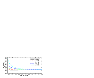
Figure 2: The mass with variations of the Borel parameter $M^{2}$ and threshold parameter $s_{0}$. The notations $\alpha$, $\beta$, $\gamma$, $\lambda$, $\tau$ and $\xi$ correspond to the threshold parameters $s_{0}=26\,\rm{GeV}^{2}$, $27\,\rm{GeV}^{2}$, $28\,\rm{GeV}^{2}$, $29\,\rm{GeV}^{2}$, $30\,\rm{GeV}^{2}$ and $31\,\rm{GeV}^{2}$, respectively. Here we take the central values of the input parameters.

In Fig.3, we plot the contribution from the pole term with variations of the threshold parameter $s_{0}$. From the figure, we can see that the value $s_{0}\leq 27\,\rm{GeV}^{2}$ is too small to satisfy the pole dominance condition. If we take the values $s_{0}=(28-30)\,\rm{GeV}^{2}$ and $M^{2}=(3.0-3.6)\,\rm{GeV}^{2}$, the pole contribution is about $(44-68)\%$, the pole dominance condition is well satisfied. The Borel window changes with variations of the threshold parameter $s_{0}$, in this article, the Borel window is taken as $0.6\,\rm{GeV}^{2}$, which is small enough. If we take larger threshold parameter, the Borel window is larger and the resulting mass is larger, see Fig.2. In this article, we intend to obtain the possibly lowest mass which is supposed to be the ground state mass by imposing the two criteria of the QCD sum rules. In the Borel window $M^{2}=(3.0-3.6)\,\rm{GeV}^{2}$, the main contributions come from the perturbative term $+$ the ⟨s¯​s⟩delimited-βŸ¨βŸ©Β―π‘ π‘ \langle\bar{s}s\rangle term $+$ the ⟨s¯​gs​σ​G​s⟩delimited-βŸ¨βŸ©Β―π‘ subscriptπ‘”π‘ πœŽπΊπ‘ \langle\bar{s}g_{s}\sigma Gs\rangle term, while the dominating one is the perturbative term, the convergent behavior in the operator product expansion is very good, see Fig.1.

Refer to caption
Figure 3: The contribution from the pole term with variations of the Borel parameter $M^{2}$ and threshold parameter $s_{0}$. The notations $\alpha$, $\beta$, $\gamma$, $\lambda$, $\tau$ and $\xi$ correspond to the threshold parameters $s_{0}=26\,\rm{GeV}^{2}$, $27\,\rm{GeV}^{2}$, $28\,\rm{GeV}^{2}$, $29\,\rm{GeV}^{2}$, $30\,\rm{GeV}^{2}$ and $31\,\rm{GeV}^{2}$, respectively. Here we take the central values of the input parameters.

Taking into account all uncertainties of the input parameters, finally we obtain the values of the mass and pole residue of the $Y(4274)$, which are shown in Figs.4-5,

$\displaystyle M_{Y}$ $\displaystyle=$ $\displaystyle 5.08^{+0.57}_{-0.24}\,\rm{GeV}\,,$
$\displaystyle\lambda_{Y}$ $\displaystyle=$ $\displaystyle 5.68^{+6.05}_{-1.39}\times 10^{-2}\,\rm{GeV}^{5}\,.$ (17)

From Fig.5, we can see that at the value $M^{2}=3\,\rm{GeV}^{2}$, the uncertainty of the pole residue is too large, the platform is not flat enough, we can take a smaller Borel window, $M^{2}=(3.2-3.6)\,\rm{GeV}^{2}$, then

$\displaystyle M_{Y}$ $\displaystyle=$ $\displaystyle 5.06^{+0.41}_{-0.22}\,\rm{GeV}\,,$
$\displaystyle\lambda_{Y}$ $\displaystyle=$ $\displaystyle 5.56^{+3.02}_{-1.27}\times 10^{-2}\,\rm{GeV}^{5}\,.$ (18)

In the QCD sum rules, the high dimension vacuum condensates are always factorized to lower condensates with vacuum saturation, factorization works well in large $N_{c}$ limit. In the real world, $N_{c}=3$, there are deviations from the factorable formula, we can introduce a factor $\kappa$ to parameterize the deviations,

⟨s¯​s⟩2,⟨s¯​sβŸ©β€‹βŸ¨s¯​gs​σ​G​s⟩,⟨s¯​gs​σ​G​s⟩2superscriptdelimited-βŸ¨βŸ©Β―π‘ π‘ 2delimited-βŸ¨βŸ©Β―π‘ π‘ delimited-βŸ¨βŸ©Β―π‘ subscriptπ‘”π‘ πœŽπΊπ‘ superscriptdelimited-βŸ¨βŸ©Β―π‘ subscriptπ‘”π‘ πœŽπΊπ‘ 2\displaystyle\langle\bar{s}s\rangle^{2}\,,\,\langle\bar{s}s\rangle\langle\bar{s}g_{s}\sigma Gs\rangle\,,\,\langle\bar{s}g_{s}\sigma Gs\rangle^{2} $\displaystyle\rightarrow$ ΞΊβ€‹βŸ¨s¯​s⟩2,ΞΊβ€‹βŸ¨s¯​sβŸ©β€‹βŸ¨s¯​gs​σ​G​s⟩,ΞΊβ€‹βŸ¨s¯​gs​σ​G​s⟩2.πœ…superscriptdelimited-βŸ¨βŸ©Β―π‘ π‘ 2πœ…delimited-βŸ¨βŸ©Β―π‘ π‘ delimited-βŸ¨βŸ©Β―π‘ subscriptπ‘”π‘ πœŽπΊπ‘ πœ…superscriptdelimited-βŸ¨βŸ©Β―π‘ subscriptπ‘”π‘ πœŽπΊπ‘ 2\displaystyle\kappa\langle\bar{s}s\rangle^{2}\,,\,\kappa\langle\bar{s}s\rangle\langle\bar{s}g_{s}\sigma Gs\rangle\,,\,\kappa\langle\bar{s}g_{s}\sigma Gs\rangle^{2}\,. (19)

In Fig.6, we plot the mass $M_{Y}$ with variations of the parameter $\kappa$ at the interval $\kappa=0-2$. From the figure, we can see that the value of the $M_{Y}$ changes quickly at the region $M^{2}\leq 3.0\,\rm{GeV}^{2}$, and increases with the $\kappa$ monotonously. At the interval $M^{2}=(3.2-3.6)\,\rm{GeV}^{2}$, the value $\kappa=1\pm 1$ leads to an uncertainty about ${}^{+0.32}_{-0.17}\,\rm{GeV}$, which is too small to smear the discrepancy between the present prediction ($5.06\,\rm{GeV}$) and the experimental data ($4.274\,\rm{GeV}$) [9]. In the QCD sum rules for the masses of the $\rho$ meson and nucleon, $\kappa\geq 1$ [21]. If the same value holds for the molecular states, the deviation from the factorable formula means even larger discrepancy between the present prediction and the experimental data.

The central value $M_{Y}=5.06\,\rm{GeV}$ is about $770\,\rm{MeV}$ above the $\bar{D}_{s}D_{s0}(2317)$ threshold [13], the $\bar{D}_{s}D_{s0}(2317)$ is probably a virtual state and not related to the charmonium-like state $Y(4274)$. The present prediction is considerably larger than the value $M_{\bar{D}_{s}{D}_{s0}}=(4.78\pm 0.54)\,\rm{GeV}$ [12]. In Ref.[12], Finazzo, Liu and Nielsen take the threshold parameter as $s_{0}=(M_{Y}+0.5\,\rm{GeV})^{2}$, and adjust the threshold parameter and Borel parameter to obtain the Borel window and reproduce the relation $s_{0}=\left(M_{Y}+(0.4\sim 0.6)\,\rm{GeV}\right)^{2}$. While in the present work, we search for the threshold parameter and Borel parameter by imposing the two criteria of the QCD sum rules, and try to obtain the ground state mass (which is not necessarily the same as $M_{Y}$) in the Borel window, as the tetraquark states, irrespective of the molecule type and the diquark-antidiquark type, have not been firmly established yet, and we have no confidence to take the ground state as the $Y(4274)$.

The flux-tube model [22], the lattice QCD [23] and the QCD string model [24] predict that the masses of the low lying hybrid charmonia are about $(4.0-4.2)\,\rm{GeV}$, $(4.0-4.4)\,\rm{GeV}$ and $(4.2-4.5)\,\rm{GeV}$, respectively, which are consistent with the experimental data. While the QCD sum rules indicate that the masses of the ground-state hybrid charmonia with $J^{PC}=0^{++}$, $0^{--}$ and $1^{+-}$ are $5.4\,\rm{GeV}$, $5.8\,\rm{GeV}$ and $4.3\,\rm{GeV}$, respectively [25], which disfavors identifying the $Y(4274)$ as the $0^{++}$ hybrid charmonium because the CDF collaboration fitted the experimental data to an $S$-wave Breit-Wigner resonance [9].

The hybrid mesons usually decay to an $S$-wave and a $P$-wave meson pair, and the couplings to two $S$-wave mesons are suppressed [26]. If the $Y(4274)$ is a hybrid charmonium, the decay $Y(4274)\to J/\psi\phi$ can take place through the final-state re-scattering mechanism, $Y(4274)\to D_{s}\bar{D}_{s0}(2317)\to J/\psi\phi$, and the decay to two photons should be forbidden or very small [27], which is in contrary to the $X(4350)$ observed by the Belle collaboration in the $\phi J/\psi$ invariant mass distributions in the process $\gamma\gamma\to\phi J/\psi$ [8]. The $X(4350)$ has been tentatively identified as the $2^{++}$ $cs\overline{cs}$ tetraquark state [3, 8], the (or not the) $D_{s}^{*}\bar{D}_{s0}$ molecular state ([28]) [8, 29, 30] , the $P$-wave charmonium $\chi_{c2}^{\prime\prime}$ [31], the scalar $cs\overline{cs}$ tetraquark state [32, 33], the scalar c¯​cβˆ’Dsβˆ—β€‹DΒ―sβˆ—Β―π‘π‘superscriptsubscriptπ·π‘ βˆ—superscriptsubscriptΒ―π·π‘ βˆ—\bar{c}c-{D}_{s}^{\ast}{\bar{D}}_{s}^{\ast} mixing state [32], etc.

In Ref.[34], we study the mass spectrum of the scalar hidden charmed and hidden bottom tetraquark states in a systematic way using the QCD sum rules, and observe that the scalar-scalar type and axial-vector-axial-vector type scalar $cs\bar{c}\bar{s}$ tetraquark states have the lowest masses, about $(4.44\pm 0.16)\,\rm{GeV}$, while the pseudoscalar $cs\bar{c}\bar{s}$ tetraquark states have much larger masses. The $Y(4274)$ may also be an scalar $cs\bar{c}\bar{s}$ tetraquark state, and decay $Y(4274)\to J/\psi\phi$ takes place through fall-apart mechanism with rearrangement in the color space. More experimental data are still needed to identify the new charmonium-like states.

Refer to caption
Figure 4: The mass with variations of the Borel parameter $M^{2}$.
Refer to caption
Figure 5: The pole residue with variations of the Borel parameter $M^{2}$.
Refer to caption
Figure 6: The mass with variations of the parameters $\kappa$ and $M^{2}$, other parameters are taken to be the central values.

4 Conclusion

In this article, we assume that there exists a pseudoscalar $\bar{D}_{s}D_{s0}(2317)$ (or $D_{s}{\bar{D}}_{s0}(2317)$) molecular state in the $J/\psi\phi$ invariant mass distribution indeed, and study its mass with the molecule-type interpolating current in details using the QCD sum rules. The numerical result indicates that the mass is about $M_{Y}=5.06^{+0.41}_{-0.22}\,\rm{GeV}$, which is inconsistent with the experimental data. The $\bar{D}_{s}D_{s0}(2317)$ (or $D_{s}{\bar{D}}_{s0}(2317)$) is probably a virtual state and not related to the charmonium-like state $Y(4274)$, and we cannot draw a definite conclusion with the QCD sum rules alone.

Acknowledgements

This work is supported by National Natural Science Foundation, Grant Number 11075053, and the Fundamental Research Funds for the Central Universities.

Appendix

The spectral densities at the level of the quark-gluon degrees of freedom:

$\displaystyle\rho_{0}(s)$ $\displaystyle=$ $\displaystyle\frac{3}{2048\pi^{6}}\int_{\alpha_{i}}^{\alpha_{f}}d\alpha\int_{\beta_{i}}^{1-\alpha}d\beta\alpha\beta(1-\alpha-\beta)^{3}(s-\widetilde{m}^{2}_{c})^{2}(7s^{2}-6s\widetilde{m}^{2}_{c}+\widetilde{m}^{4}_{c})\,,$ (20)
ρ⟨s¯​sβŸ©β€‹(s)subscript𝜌delimited-βŸ¨βŸ©Β―π‘ π‘ π‘ \displaystyle\rho_{\langle\bar{s}s\rangle}(s) $\displaystyle=$ 3​msβ€‹βŸ¨s¯​s⟩64​π4β€‹βˆ«Ξ±iΞ±fπ‘‘Ξ±β€‹βˆ«Ξ²i1βˆ’Ξ±π‘‘Ξ²β€‹Ξ±β€‹Ξ²β€‹(1βˆ’Ξ±βˆ’Ξ²)​(10​s2βˆ’12​s​m~c2+3​m~c4)3subscriptπ‘šπ‘ delimited-βŸ¨βŸ©Β―π‘ π‘ 64superscriptπœ‹4superscriptsubscriptsubscript𝛼𝑖subscript𝛼𝑓differential-d𝛼superscriptsubscriptsubscript𝛽𝑖1𝛼differential-d𝛽𝛼𝛽1𝛼𝛽10superscript𝑠212𝑠subscriptsuperscript~π‘š2𝑐3subscriptsuperscript~π‘š4𝑐\displaystyle\frac{3m_{s}\langle\bar{s}s\rangle}{64\pi^{4}}\int_{\alpha_{i}}^{\alpha_{f}}d\alpha\int_{\beta_{i}}^{1-\alpha}d\beta\alpha\beta(1-\alpha-\beta)(10s^{2}-12s\widetilde{m}^{2}_{c}+3\widetilde{m}^{4}_{c}) (21)
βˆ’msβ€‹βŸ¨s¯​gs​σ​G​s⟩128​π4β€‹βˆ«Ξ±iΞ±fπ‘‘Ξ±β€‹βˆ«Ξ²i1βˆ’Ξ±π‘‘Ξ²β€‹Ξ±β€‹Ξ²β€‹[6​(2​sβˆ’m~c2)+s2​δ​(sβˆ’m~c2)]subscriptπ‘šπ‘ delimited-βŸ¨βŸ©Β―π‘ subscriptπ‘”π‘ πœŽπΊπ‘ 128superscriptπœ‹4superscriptsubscriptsubscript𝛼𝑖subscript𝛼𝑓differential-d𝛼superscriptsubscriptsubscript𝛽𝑖1𝛼differential-d𝛽𝛼𝛽delimited-[]62𝑠subscriptsuperscript~π‘š2𝑐superscript𝑠2𝛿𝑠subscriptsuperscript~π‘š2𝑐\displaystyle-\frac{m_{s}\langle\bar{s}g_{s}\sigma Gs\rangle}{128\pi^{4}}\int_{\alpha_{i}}^{\alpha_{f}}d\alpha\int_{\beta_{i}}^{1-\alpha}d\beta\alpha\beta\left[6(2s-\widetilde{m}^{2}_{c})+s^{2}\delta(s-\widetilde{m}^{2}_{c})\right]
+3​ms​mc2β€‹βŸ¨s¯​s⟩32​π4β€‹βˆ«Ξ±iΞ±fπ‘‘Ξ±β€‹βˆ«Ξ²i1βˆ’Ξ±π‘‘Ξ²β€‹(sβˆ’m~c2)3subscriptπ‘šπ‘ superscriptsubscriptπ‘šπ‘2delimited-βŸ¨βŸ©Β―π‘ π‘ 32superscriptπœ‹4superscriptsubscriptsubscript𝛼𝑖subscript𝛼𝑓differential-d𝛼superscriptsubscriptsubscript𝛽𝑖1𝛼differential-d𝛽𝑠subscriptsuperscript~π‘š2𝑐\displaystyle+\frac{3m_{s}m_{c}^{2}\langle\bar{s}s\rangle}{32\pi^{4}}\int_{\alpha_{i}}^{\alpha_{f}}d\alpha\int_{\beta_{i}}^{1-\alpha}d\beta(s-\widetilde{m}^{2}_{c})
+3​msβ€‹βŸ¨s¯​gs​σ​G​s⟩128​π4β€‹βˆ«Ξ±iΞ±fπ‘‘Ξ±β€‹βˆ«Ξ²i1βˆ’Ξ±π‘‘Ξ²β€‹m~c2βˆ’3​ms​mc2β€‹βŸ¨s¯​gs​σ​G​s⟩128​π4β€‹βˆ«Ξ±iΞ±f𝑑α,3subscriptπ‘šπ‘ delimited-βŸ¨βŸ©Β―π‘ subscriptπ‘”π‘ πœŽπΊπ‘ 128superscriptπœ‹4superscriptsubscriptsubscript𝛼𝑖subscript𝛼𝑓differential-d𝛼superscriptsubscriptsubscript𝛽𝑖1𝛼differential-d𝛽subscriptsuperscript~π‘š2𝑐3subscriptπ‘šπ‘ superscriptsubscriptπ‘šπ‘2delimited-βŸ¨βŸ©Β―π‘ subscriptπ‘”π‘ πœŽπΊπ‘ 128superscriptπœ‹4superscriptsubscriptsubscript𝛼𝑖subscript𝛼𝑓differential-d𝛼\displaystyle+\frac{3m_{s}\langle\bar{s}g_{s}\sigma Gs\rangle}{128\pi^{4}}\int_{\alpha_{i}}^{\alpha_{f}}d\alpha\int_{\beta_{i}}^{1-\alpha}d\beta\widetilde{m}^{2}_{c}-\frac{3m_{s}m_{c}^{2}\langle\bar{s}g_{s}\sigma Gs\rangle}{128\pi^{4}}\int_{\alpha_{i}}^{\alpha_{f}}d\alpha\,,
ρ⟨s¯​s⟩2​(s)subscript𝜌superscriptdelimited-βŸ¨βŸ©Β―π‘ π‘ 2𝑠\displaystyle\rho_{\langle\bar{s}s\rangle^{2}}(s) $\displaystyle=$ βˆ’mc2β€‹βŸ¨s¯​s⟩216​π2β€‹βˆ«Ξ±iΞ±fπ‘‘Ξ±βˆ’βŸ¨s¯​gs​σ​G​s⟩264​π2​M2β€‹βˆ«Ξ±iΞ±f𝑑α​[sβˆ’s22​M2+α​(1βˆ’Ξ±)​s34​M4]superscriptsubscriptπ‘šπ‘2superscriptdelimited-βŸ¨βŸ©Β―π‘ π‘ 216superscriptπœ‹2superscriptsubscriptsubscript𝛼𝑖subscript𝛼𝑓differential-d𝛼superscriptdelimited-βŸ¨βŸ©Β―π‘ subscriptπ‘”π‘ πœŽπΊπ‘ 264superscriptπœ‹2superscript𝑀2superscriptsubscriptsubscript𝛼𝑖subscript𝛼𝑓differential-d𝛼delimited-[]𝑠superscript𝑠22superscript𝑀2𝛼1𝛼superscript𝑠34superscript𝑀4\displaystyle-\frac{m_{c}^{2}\langle\bar{s}s\rangle^{2}}{16\pi^{2}}\int_{\alpha_{i}}^{\alpha_{f}}d\alpha-\frac{\langle\bar{s}g_{s}\sigma Gs\rangle^{2}}{64\pi^{2}M^{2}}\int_{\alpha_{i}}^{\alpha_{f}}d\alpha\left[s-\frac{s^{2}}{2M^{2}}+\frac{\alpha(1-\alpha)s^{3}}{4M^{4}}\right]
δ​(sβˆ’m~~c2)+mc2β€‹βŸ¨s¯​sβŸ©β€‹βŸ¨s¯​gs​σ​G​s⟩32​π2β€‹βˆ«Ξ±iΞ±f𝑑α​[1βˆ’1α​(1βˆ’Ξ±)+sM2]​δ​(sβˆ’m~~c2),𝛿𝑠superscriptsubscript~~π‘šπ‘2superscriptsubscriptπ‘šπ‘2delimited-βŸ¨βŸ©Β―π‘ π‘ delimited-βŸ¨βŸ©Β―π‘ subscriptπ‘”π‘ πœŽπΊπ‘ 32superscriptπœ‹2superscriptsubscriptsubscript𝛼𝑖subscript𝛼𝑓differential-d𝛼delimited-[]11𝛼1𝛼𝑠superscript𝑀2𝛿𝑠superscriptsubscript~~π‘šπ‘2\displaystyle\delta(s-\widetilde{\widetilde{m}}_{c}^{2})+\frac{m_{c}^{2}\langle\bar{s}s\rangle\langle\bar{s}g_{s}\sigma Gs\rangle}{32\pi^{2}}\int_{\alpha_{i}}^{\alpha_{f}}d\alpha\left[1-\frac{1}{\alpha(1-\alpha)}+\frac{s}{M^{2}}\right]\delta(s-\widetilde{\widetilde{m}}_{c}^{2})\,,
ρ⟨G​G⟩A​(s)subscriptsuperscript𝜌𝐴delimited-βŸ¨βŸ©πΊπΊπ‘ \displaystyle\rho^{A}_{\langle GG\rangle}(s) $\displaystyle=$ $\displaystyle-\frac{m_{c}^{2}}{512\pi^{4}}\int_{\alpha_{i}}^{\alpha_{f}}d\alpha\int_{\beta_{i}}^{1-\alpha}d\beta\left(\frac{\alpha}{\beta^{2}}+\frac{\beta}{\alpha^{2}}\right)(1-\alpha-\beta)^{3}\left[2s-\widetilde{m}^{2}_{c}+\frac{s^{2}}{6}\delta(s-\widetilde{m}^{2}_{c})\right]$ (23)
$\displaystyle+\frac{3}{1024\pi^{4}}\int_{\alpha_{i}}^{\alpha_{f}}d\alpha\int_{\beta_{i}}^{1-\alpha}d\beta(\alpha+\beta)(1-\alpha-\beta)^{2}(10s^{2}-12s\widetilde{m}^{2}_{c}+3\widetilde{m}^{4}_{c})$
βˆ’ms​mc2β€‹βŸ¨s¯​s⟩192​π2β€‹βˆ«Ξ±iΞ±fπ‘‘Ξ±β€‹βˆ«Ξ²i1βˆ’Ξ±π‘‘Ξ²β€‹(Ξ±Ξ²2+Ξ²Ξ±2)​(1βˆ’Ξ±βˆ’Ξ²)​[1+sM2+s22​M4]​δ​(sβˆ’m~c2)subscriptπ‘šπ‘ superscriptsubscriptπ‘šπ‘2delimited-βŸ¨βŸ©Β―π‘ π‘ 192superscriptπœ‹2superscriptsubscriptsubscript𝛼𝑖subscript𝛼𝑓differential-d𝛼superscriptsubscriptsubscript𝛽𝑖1𝛼differential-d𝛽𝛼superscript𝛽2𝛽superscript𝛼21𝛼𝛽delimited-[]1𝑠superscript𝑀2superscript𝑠22superscript𝑀4𝛿𝑠subscriptsuperscript~π‘š2𝑐\displaystyle-\frac{m_{s}m_{c}^{2}\langle\bar{s}s\rangle}{192\pi^{2}}\int_{\alpha_{i}}^{\alpha_{f}}d\alpha\int_{\beta_{i}}^{1-\alpha}d\beta\left(\frac{\alpha}{\beta^{2}}+\frac{\beta}{\alpha^{2}}\right)(1-\alpha-\beta)\left[1+\frac{s}{M^{2}}+\frac{s^{2}}{2M^{4}}\right]\delta(s-\widetilde{m}^{2}_{c})
+ms​mc2β€‹βŸ¨s¯​gs​σ​G​s⟩2304​π2​M6β€‹βˆ«Ξ±iΞ±fπ‘‘Ξ±β€‹βˆ«Ξ²i1βˆ’Ξ±π‘‘Ξ²β€‹(Ξ±Ξ²2+Ξ²Ξ±2)​s2​δ​(sβˆ’m~c2)subscriptπ‘šπ‘ superscriptsubscriptπ‘šπ‘2delimited-βŸ¨βŸ©Β―π‘ subscriptπ‘”π‘ πœŽπΊπ‘ 2304superscriptπœ‹2superscript𝑀6superscriptsubscriptsubscript𝛼𝑖subscript𝛼𝑓differential-d𝛼superscriptsubscriptsubscript𝛽𝑖1𝛼differential-d𝛽𝛼superscript𝛽2𝛽superscript𝛼2superscript𝑠2𝛿𝑠subscriptsuperscript~π‘š2𝑐\displaystyle+\frac{m_{s}m_{c}^{2}\langle\bar{s}g_{s}\sigma Gs\rangle}{2304\pi^{2}M^{6}}\int_{\alpha_{i}}^{\alpha_{f}}d\alpha\int_{\beta_{i}}^{1-\alpha}d\beta\left(\frac{\alpha}{\beta^{2}}+\frac{\beta}{\alpha^{2}}\right)s^{2}\delta(s-\widetilde{m}^{2}_{c})
βˆ’ms​mc4β€‹βŸ¨s¯​s⟩192​π2​M2β€‹βˆ«Ξ±iΞ±fπ‘‘Ξ±β€‹βˆ«Ξ²i1βˆ’Ξ±π‘‘Ξ²β€‹(1Ξ±3+1Ξ²3)​δ​(sβˆ’m~c2)subscriptπ‘šπ‘ superscriptsubscriptπ‘šπ‘4delimited-βŸ¨βŸ©Β―π‘ π‘ 192superscriptπœ‹2superscript𝑀2superscriptsubscriptsubscript𝛼𝑖subscript𝛼𝑓differential-d𝛼superscriptsubscriptsubscript𝛽𝑖1𝛼differential-d𝛽1superscript𝛼31superscript𝛽3𝛿𝑠subscriptsuperscript~π‘š2𝑐\displaystyle-\frac{m_{s}m_{c}^{4}\langle\bar{s}s\rangle}{192\pi^{2}M^{2}}\int_{\alpha_{i}}^{\alpha_{f}}d\alpha\int_{\beta_{i}}^{1-\alpha}d\beta\left(\frac{1}{\alpha^{3}}+\frac{1}{\beta^{3}}\right)\delta(s-\widetilde{m}^{2}_{c})
+ms​mc2β€‹βŸ¨s¯​s⟩64​π2β€‹βˆ«Ξ±iΞ±fπ‘‘Ξ±β€‹βˆ«Ξ²i1βˆ’Ξ±π‘‘Ξ²β€‹(1Ξ±2+1Ξ²2)​δ​(sβˆ’m~c2)subscriptπ‘šπ‘ superscriptsubscriptπ‘šπ‘2delimited-βŸ¨βŸ©Β―π‘ π‘ 64superscriptπœ‹2superscriptsubscriptsubscript𝛼𝑖subscript𝛼𝑓differential-d𝛼superscriptsubscriptsubscript𝛽𝑖1𝛼differential-d𝛽1superscript𝛼21superscript𝛽2𝛿𝑠subscriptsuperscript~π‘š2𝑐\displaystyle+\frac{m_{s}m_{c}^{2}\langle\bar{s}s\rangle}{64\pi^{2}}\int_{\alpha_{i}}^{\alpha_{f}}d\alpha\int_{\beta_{i}}^{1-\alpha}d\beta\left(\frac{1}{\alpha^{2}}+\frac{1}{\beta^{2}}\right)\delta(s-\widetilde{m}^{2}_{c})
+msβ€‹βŸ¨s¯​s⟩128​π2β€‹βˆ«Ξ±iΞ±fπ‘‘Ξ±β€‹βˆ«Ξ²i1βˆ’Ξ±π‘‘Ξ²β€‹(Ξ±+Ξ²)​[3+(2​s+s22​M2)​δ​(sβˆ’m~c2)]subscriptπ‘šπ‘ delimited-βŸ¨βŸ©Β―π‘ π‘ 128superscriptπœ‹2superscriptsubscriptsubscript𝛼𝑖subscript𝛼𝑓differential-d𝛼superscriptsubscriptsubscript𝛽𝑖1𝛼differential-d𝛽𝛼𝛽delimited-[]32𝑠superscript𝑠22superscript𝑀2𝛿𝑠subscriptsuperscript~π‘š2𝑐\displaystyle+\frac{m_{s}\langle\bar{s}s\rangle}{128\pi^{2}}\int_{\alpha_{i}}^{\alpha_{f}}d\alpha\int_{\beta_{i}}^{1-\alpha}d\beta(\alpha+\beta)\left[3+\left(2s+\frac{s^{2}}{2M^{2}}\right)\delta(s-\widetilde{m}^{2}_{c})\right]
βˆ’ms​mc4β€‹βŸ¨s¯​gs​σ​G​s⟩768​π2​M4β€‹βˆ«Ξ±iΞ±fπ‘‘Ξ±β€‹βˆ«Ξ²i1βˆ’Ξ±π‘‘Ξ²β€‹(1α​β3+1Ξ±3​β)​δ​(sβˆ’m~c2)subscriptπ‘šπ‘ superscriptsubscriptπ‘šπ‘4delimited-βŸ¨βŸ©Β―π‘ subscriptπ‘”π‘ πœŽπΊπ‘ 768superscriptπœ‹2superscript𝑀4superscriptsubscriptsubscript𝛼𝑖subscript𝛼𝑓differential-d𝛼superscriptsubscriptsubscript𝛽𝑖1𝛼differential-d𝛽1𝛼superscript𝛽31superscript𝛼3𝛽𝛿𝑠subscriptsuperscript~π‘š2𝑐\displaystyle-\frac{m_{s}m_{c}^{4}\langle\bar{s}g_{s}\sigma Gs\rangle}{768\pi^{2}M^{4}}\int_{\alpha_{i}}^{\alpha_{f}}d\alpha\int_{\beta_{i}}^{1-\alpha}d\beta\left(\frac{1}{\alpha\beta^{3}}+\frac{1}{\alpha^{3}\beta}\right)\delta(s-\widetilde{m}^{2}_{c})
+ms​mc2β€‹βŸ¨s¯​gs​σ​G​s⟩256​π2​M2β€‹βˆ«Ξ±iΞ±fπ‘‘Ξ±β€‹βˆ«Ξ²i1βˆ’Ξ±π‘‘Ξ²β€‹(1α​β2+1Ξ±2​β)​δ​(sβˆ’m~c2),subscriptπ‘šπ‘ superscriptsubscriptπ‘šπ‘2delimited-βŸ¨βŸ©Β―π‘ subscriptπ‘”π‘ πœŽπΊπ‘ 256superscriptπœ‹2superscript𝑀2superscriptsubscriptsubscript𝛼𝑖subscript𝛼𝑓differential-d𝛼superscriptsubscriptsubscript𝛽𝑖1𝛼differential-d𝛽1𝛼superscript𝛽21superscript𝛼2𝛽𝛿𝑠subscriptsuperscript~π‘š2𝑐\displaystyle+\frac{m_{s}m_{c}^{2}\langle\bar{s}g_{s}\sigma Gs\rangle}{256\pi^{2}M^{2}}\int_{\alpha_{i}}^{\alpha_{f}}d\alpha\int_{\beta_{i}}^{1-\alpha}d\beta\left(\frac{1}{\alpha\beta^{2}}+\frac{1}{\alpha^{2}\beta}\right)\delta(s-\widetilde{m}^{2}_{c})\,,
ρ⟨G​G⟩B​(s)subscriptsuperscript𝜌𝐡delimited-βŸ¨βŸ©πΊπΊπ‘ \displaystyle\rho^{B}_{\langle GG\rangle}(s) $\displaystyle=$ mc4β€‹βŸ¨s¯​s⟩2288​M4β€‹βˆ«Ξ±iΞ±f𝑑α​[1Ξ±3+1(1βˆ’Ξ±)3]​δ​(sβˆ’m~~c2)superscriptsubscriptπ‘šπ‘4superscriptdelimited-βŸ¨βŸ©Β―π‘ π‘ 2288superscript𝑀4superscriptsubscriptsubscript𝛼𝑖subscript𝛼𝑓differential-d𝛼delimited-[]1superscript𝛼31superscript1𝛼3𝛿𝑠superscriptsubscript~~π‘šπ‘2\displaystyle\frac{m_{c}^{4}\langle\bar{s}s\rangle^{2}}{288M^{4}}\int_{\alpha_{i}}^{\alpha_{f}}d\alpha\left[\frac{1}{\alpha^{3}}+\frac{1}{(1-\alpha)^{3}}\right]\delta(s-\widetilde{\widetilde{m}}_{c}^{2}) (24)
+ms​mc4β€‹βŸ¨s¯​gs​σ​G​s⟩768​π2​M4β€‹βˆ«Ξ±iΞ±f𝑑α​[1Ξ±3+1(1βˆ’Ξ±)3]​δ​(sβˆ’m~~c2)subscriptπ‘šπ‘ superscriptsubscriptπ‘šπ‘4delimited-βŸ¨βŸ©Β―π‘ subscriptπ‘”π‘ πœŽπΊπ‘ 768superscriptπœ‹2superscript𝑀4superscriptsubscriptsubscript𝛼𝑖subscript𝛼𝑓differential-d𝛼delimited-[]1superscript𝛼31superscript1𝛼3𝛿𝑠superscriptsubscript~~π‘šπ‘2\displaystyle+\frac{m_{s}m_{c}^{4}\langle\bar{s}g_{s}\sigma Gs\rangle}{768\pi^{2}M^{4}}\int_{\alpha_{i}}^{\alpha_{f}}d\alpha\left[\frac{1}{\alpha^{3}}+\frac{1}{(1-\alpha)^{3}}\right]\delta(s-\widetilde{\widetilde{m}}_{c}^{2})
βˆ’mc2β€‹βŸ¨s¯​s⟩296​M2β€‹βˆ«Ξ±iΞ±f𝑑α​[1Ξ±2+1(1βˆ’Ξ±)2]​δ​(sβˆ’m~~c2)superscriptsubscriptπ‘šπ‘2superscriptdelimited-βŸ¨βŸ©Β―π‘ π‘ 296superscript𝑀2superscriptsubscriptsubscript𝛼𝑖subscript𝛼𝑓differential-d𝛼delimited-[]1superscript𝛼21superscript1𝛼2𝛿𝑠superscriptsubscript~~π‘šπ‘2\displaystyle-\frac{m_{c}^{2}\langle\bar{s}s\rangle^{2}}{96M^{2}}\int_{\alpha_{i}}^{\alpha_{f}}d\alpha\left[\frac{1}{\alpha^{2}}+\frac{1}{(1-\alpha)^{2}}\right]\delta(s-\widetilde{\widetilde{m}}_{c}^{2})
βˆ’ms​mc2β€‹βŸ¨s¯​gs​σ​G​s⟩256​π2​M2β€‹βˆ«Ξ±iΞ±f𝑑α​[1Ξ±2+1(1βˆ’Ξ±)2]​δ​(sβˆ’m~~c2)subscriptπ‘šπ‘ superscriptsubscriptπ‘šπ‘2delimited-βŸ¨βŸ©Β―π‘ subscriptπ‘”π‘ πœŽπΊπ‘ 256superscriptπœ‹2superscript𝑀2superscriptsubscriptsubscript𝛼𝑖subscript𝛼𝑓differential-d𝛼delimited-[]1superscript𝛼21superscript1𝛼2𝛿𝑠superscriptsubscript~~π‘šπ‘2\displaystyle-\frac{m_{s}m_{c}^{2}\langle\bar{s}g_{s}\sigma Gs\rangle}{256\pi^{2}M^{2}}\int_{\alpha_{i}}^{\alpha_{f}}d\alpha\left[\frac{1}{\alpha^{2}}+\frac{1}{(1-\alpha)^{2}}\right]\delta(s-\widetilde{\widetilde{m}}_{c}^{2})
βˆ’msβ€‹βŸ¨s¯​gs​σ​G​s⟩768​π2β€‹βˆ«Ξ±iΞ±f𝑑α​[1+sM2+s22​M4]​δ​(sβˆ’m~~c2),subscriptπ‘šπ‘ delimited-βŸ¨βŸ©Β―π‘ subscriptπ‘”π‘ πœŽπΊπ‘ 768superscriptπœ‹2superscriptsubscriptsubscript𝛼𝑖subscript𝛼𝑓differential-d𝛼delimited-[]1𝑠superscript𝑀2superscript𝑠22superscript𝑀4𝛿𝑠superscriptsubscript~~π‘šπ‘2\displaystyle-\frac{m_{s}\langle\bar{s}g_{s}\sigma Gs\rangle}{768\pi^{2}}\int_{\alpha_{i}}^{\alpha_{f}}d\alpha\left[1+\frac{s}{M^{2}}+\frac{s^{2}}{2M^{4}}\right]\delta(s-\widetilde{\widetilde{m}}_{c}^{2})\,,
ρ⟨G​G​GβŸ©β€‹(s)subscript𝜌delimited-βŸ¨βŸ©πΊπΊπΊπ‘ \displaystyle\rho_{\langle GGG\rangle}(s) $\displaystyle=$ $\displaystyle\frac{m_{c}^{2}}{4096\pi^{6}}\int_{\alpha_{i}}^{\alpha_{f}}d\alpha\int_{\beta_{i}}^{1-\alpha}d\beta\left(\frac{\alpha}{\beta^{3}}+\frac{\beta}{\alpha^{3}}\right)(1-\alpha-\beta)^{3}\left[1+\left(\frac{2s}{3}+\frac{s^{2}}{6M^{2}}\right)\delta(s-\widetilde{m}^{2}_{c})\right]$
$\displaystyle-\frac{1}{8192\pi^{6}}\int_{\alpha_{i}}^{\alpha_{f}}d\alpha\int_{\beta_{i}}^{1-\alpha}d\beta\left(\frac{\alpha}{\beta^{2}}+\frac{\beta}{\alpha^{2}}\right)(1-\alpha-\beta)^{3}\left[2s-\widetilde{m}^{2}_{c}+\frac{s^{2}}{6}\delta(s-\widetilde{m}^{2}_{c})\right]$
$\displaystyle+\frac{3}{8192\pi^{6}}\int_{\alpha_{i}}^{\alpha_{f}}d\alpha\int_{\beta_{i}}^{1-\alpha}d\beta\left(\frac{\alpha}{\beta}+\frac{\beta}{\alpha}\right)(1-\alpha-\beta)^{2}\left[6s-3\widetilde{m}^{2}_{c}+\frac{s^{2}}{2}\delta(s-\widetilde{m}^{2}_{c})\right]$
$\displaystyle-\frac{m_{c}^{2}}{4096\pi^{6}}\int_{\alpha_{i}}^{\alpha_{f}}d\alpha\int_{\beta_{i}}^{1-\alpha}d\beta\left(\frac{\alpha}{\beta^{2}}+\frac{\beta}{\alpha^{2}}\right)(1-\alpha-\beta)^{2}\left[3+\left(2s+\frac{s^{2}}{2M^{2}}\right)\delta(s-\widetilde{m}^{2}_{c})\right]\,,$

where $\alpha_{f}=\frac{1+\sqrt{1-\frac{4m_{c}^{2}}{s}}}{2}$, $\alpha_{i}=\frac{1-\sqrt{1-\frac{4m_{c}^{2}}{s}}}{2}$, $\beta_{i}=\frac{\alpha m_{c}^{2}}{\alpha s-m_{c}^{2}}$, $\widetilde{m}_{c}^{2}=\frac{(\alpha+\beta)m_{c}^{2}}{\alpha\beta}$, $\widetilde{\widetilde{m}}_{c}^{2}=\frac{m_{c}^{2}}{\alpha(1-\alpha)}$.

References

  • [1] T. Aaltonen et al, Phys. Rev. Lett. 102 (2009) 242002.
  • [2] X. Liu and S. L. Zhu, Phys. Rev. D80 (2009) 017502; T. Branz, T. Gutsche and V. E. Lyubovitskij, Phys. Rev. D80 (2009) 054019; R. M. Albuquerque, M. E. Bracco and M. Nielsen, Phys. Lett. B678 (2009) 186; G. J. Ding, Eur. Phys. J. C64 (2009) 297; J. R. Zhang and M. Q. Huang, J. Phys. G37 (2010) 025005; X. Liu and H. W. Ke, Phys. Rev. D80 (2009) 034009; R. Molina and E. Oset, Phys. Rev. D80 (2009) 114013.
  • [3] Fl. Stancu, J. Phys. G37 (2010) 075017.
  • [4] N. V. Drenska, R. Faccini and A. D. Polosa, Phys. Rev. D79 (2009) 077502.
  • [5] N. Mahajan, Phys. Lett. B679 (2009) 228.
  • [6] Z. G. Wang, Eur. Phys. J. C63 (2009) 115; Z. G. Wang, Z. C. Liu and X. H. Zhang, Eur. Phys. J. C64 (2009) 373.
  • [7] X. Liu, Phys. Lett. B680 (2009) 137; E. van Beveren and G. Rupp, arXiv:0906.2278.
  • [8] C. P. Shen et al, Phys. Rev. Lett. 104 (2010) 112004.
  • [9] T. Aaltonen et al, arXiv:1101.6058.
  • [10] X. Liu, Z. G. Luo and S. L. Zhu, arXiv:1011.1045.
  • [11] J. He and X. Liu, arXiv:1102.1127.
  • [12] S. I. Finazzo, X. Liu and M. Nielsen, arXiv:1102.2347.
  • [13] K. Nakamura et al, J. Phys. G37 (2010) 075021.
  • [14] M. A. Shifman, A. I. Vainshtein and V. I. Zakharov, Nucl. Phys. B147 (1979) 385.
  • [15] L. J. Reinders, H. Rubinstein and S. Yazaki, Phys. Rept. 127 (1985) 1.
  • [16] T. Matsuki, T. Morii and K. Seo, Prog. Theor. Phys. 124 (2010) 285.
  • [17] S. H. Lee, H. Kim and Y. Kwon, Phys. Lett. B609 (2005) 252.
  • [18] R. D. Matheus, F. S. Navarra, M. Nielsen and C. M. Zanetti, Phys. Rev. D80 (2009) 056002.
  • [19] B. L. Ioffe, Prog. Part. Nucl. Phys. 56 (2006) 232.
  • [20] P. Colangelo and A. Khodjamirian, hep-ph/0010175.
  • [21] D. B. Leinweber, Annals Phys. 254 (1997) 328.
  • [22] N. Isgur and J. E. Paton, Phys. Rev. D31 (1985) 2910; T. Barnes, F. E. Close and E. S. Swanson, Phys. Rev. D52 (1995) 5242.
  • [23] P. Lacock et al, Phys. Lett. B401 (1997) 308; C. W. Bernard et al, Phys. Rev. D56 (1997) 7039; P. Chen, Phys. Rev. D64 (2001) 034509; X. Q. Luo and Y. Liu, Phys. Rev. D74 (2006) 034502.
  • [24] Y. S. Kalashnikova and A. V. Nefediev, Phys. Rev. D77 (2008) 054025; V. Mathieu, Phys. Rev. D80 (2009) 014016.
  • [25] J. Govaerts, L. J. Reinders, H. R. Rubinstein and J. Weyers, Nucl. Phys. B258 (1985) 215.
  • [26] P. R. Page, Phys. Lett. B402 (1997) 183.
  • [27] P. R. Page, Nucl. Phys. B495 (1997) 268.
  • [28] R. M. Albuquerque, J. M. Dias and M. Nielsen, Phys. Lett. B690 (2010) 141.
  • [29] J. R. Zhang and M. Q. Huang, Commun. Theor. Phys. 54 (2010) 1075.
  • [30] Y. L. Ma, Phys. Rev. D82 (2010) 015013.
  • [31] X. Liu, Z. G. Luo and Z. F. Sun, Phys. Rev. Lett. 104 (2010) 122001.
  • [32] Z. G. Wang, Phys. Lett. B690 (2010) 403.
  • [33] M. Abud, F. Buccella and F. Tramontano, Phys. Rev. D81 (2010) 074018.
  • [34] Z. G. Wang, Eur. Phys. J. C62 (2009) 375; Z. G. Wang, Phys. Rev. D79 (2009) 094027; Z. G. Wang, Eur. Phys. J. C67 (2010) 411.