Observability of pulsar beam bending by the Sgr A* black hole

Abstract

According to some models, there may be a significant population of radio pulsars in the Galactic center. In principle, a beam from one of these pulsars could pass close to the supermassive black hole (SMBH) at the center, be deflected, and be detected by Earth telescopes. Such a configuration would be an unprecedented probe of the properties of spacetime in the moderate- to strong-field regime of the SMBH. We present here background on the problem, and approximations for the probability of detection of such beams. We conclude that detection is marginally probable with current telescopes, but that telescopes that will be operating in the near future, with an appropriate multiyear observational program, will have a good chance of detecting a beam deflected by the SMBH.

1 Introduction

Near-infrared observations of stars near our Galaxy’s central supermassive black hole (SMBH) have revealed a larger number of young, massive stars than can be explained by typical star formation models (Ghez et al., 2005; Eisenhauer et al., 2005). This “paradox of youth”(Ghez et al., 2005) has pointed to the development of a possible continuing top-heavy initial mass function (IMF) in the region near the central SMBH (Maness et al., 2007; Nayakshin & Sunyaev, 2005). A top-heavy IMF near Sgr A* would imply the existence of a large number of neutron stars in close proximity to the central SMBH. Current estimates suggest that there could be $\gtrsim 10^{4}$ neutron stars within 1 pc of Sgr A* (Muno et al., 2005) and possibly $\sim 1000$ pulsars within $\sim 0.01$ pc of Sgr A* (Pfahl & Loeb, 2004).

Theoretical predictions have also suggested a cusp of $\sim 20,000$ neutron stars in the central parsec of our Galaxy (Freitag et al., 2006; Hopman & Alexander, 2006). X-ray observations have been consistent with this number of neutron stars (Deegan & Nayakshin, 2007) but appear to have ruled out the presence of a larger number of neutron stars (e.g., 40,000). For this paper, we will take the results from Pfahl & Loeb (2004) and will assume the existence of 1000 pulsars within 0.01 pc of Sgr A*. We will also follow Pfahl & Loeb in assuming that $n(r)$, the density of pulsars as a function of distance from the Galactic center, falls off as $r^{-3/2}$, so that

$$n=\frac{3}{8\pi}\times 10^{6}\,{\rm pc}^{-3}\,(r/1\,{\rm pc})^{-3/2}\,.$$ (1)

With this assumption it will turn out that the quantity of greatest importance to our predictions is the number of pulsars at distances from the central SMBH between 0.001 pc and 0.01 pc.

In this paper we will consider the possibility that an appropriate program to monitor pulsar beams from Sgr A* would detect a beam that is strongly deflected by the central SMBH. Such a system would be of great interest, as precision timing of the radio pulses from such a system would measure the properties of the spacetime through which they propagate. Preliminary work in the case of Schwarzschild black holes, presented in Wang et al. (2009b) and Wang et al. (2009a) (hereafter Paper I and Paper II), has revealed a rich structure and multiplicity of pulses observed in such geometries; subsequent work will look at how pulse timing can be used to measure properties such as the mass and spin of the SMBH, and measure or constrain deviations in the higher multipoles of the spacetime from the predictions of general relativity. In the present paper we will focus on determining the likelihood of observing a pulsar in such a configuration. To do this we will first calculate the probability that a single pulsar, in orbit around the central SMBH, emits a signal in such a way that it is strongly deflected by the central SMBH, and reaches the Earth. From this we then infer the probability that the signal from one of the assumed number of pulsars is strongly deflected, reaches the Earth, and is detectable by radio telescopes.

The paper continues in Sec. 2 with a discussion of the model for the pulsar-SMBH system, and with assumptions about pulsar characteristics and telescope sensitivities. The heart of the paper is the method of computation of probabilities in Sec. 3. Numerical estimates of probability, based on this approach, are given in Sec. 4, and considerations for an observing program are given in Sec. 5. In Sec. 6 we conclude that an observing program, even with current radio telescopes, would have some chance of detecting strongly-bent pulsar emissions, while later generations of telescopes will significantly increase the likelihood of observing these fascinating systems.

2 Background, model, and assumptions

As a simplification in our probability estimates we take the SMBH in Sgr A* to be a Schwarzschild hole. It is essentially certain, of course, that the SMBH is rotating, but the angular momentum $J$ is currently thought to be only about half of its maximum possible value of $GM^{2}/c$ where $M$ is the mass of the SMBH (Melia et al., 2001; Genzel et al., 2003). Typically, the astrophysical properties of Kerr holes differ significantly from those of Schwarzshcild holes only when $J$ is very close to $GM^{2}/c$. Our preliminary investigations of Kerr holes, in work now underway, confirms this. While frame dragging by the black hole may slightly increase the probability of detecting beams bent in the prograde sense, and decrease the probability of retrograde-bent beams, these effects largely cancel when considering the population as a whole. Thus the Schwarzschild approximation would appear to be justified for our purposes, in which it is the average properties that are of importance.

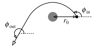
Figure 1: Photon trajectory and the definitions of the angles $\phi_{\rm in}$ and $\phi_{\rm out}=F(\phi_{\rm in};r_{0})$.

We will rely heavily on results in Papers I and II for pulsar beam deflection around a Schwarzschild hole. In those papers $\phi_{\rm in}$ is the angle between the direction of pulsar emission and the direction radially outward from the central SMBH at the emission event; the angle $\phi_{\rm out}$ is the angle between that same radial direction and the direction in which the pulsar beam is moving when it is asymptotically far from the SMBH, as sketched in Figure 1. In the absence of the bending of the beam, the two angles $\phi_{\rm in}$ and $\phi_{\rm out}$ would be equal. The effect of curvature of the beam is encoded in the function $F$ defined by

$$\phi_{\rm out}=F(\phi_{\rm in};r_{0})\,,$$ (2)

where $r_{0}$ is the distance of the emission point from the SMBH. The computational method for finding the $F$ function is discussed in Papers I and II. A practical approximation for $F$, useful for the considerations of this paper, is presented in the Appendix.

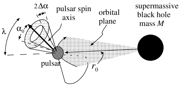
Figure 2: The geometry of the orbit, pulsar spin, and pulsar beam.

With the simplification to a nonrotating SMBH, we do not need to consider any angle between the orbit of the pulsar and the spin axis of the SMBH, The geometric parameters of interest are pictured in Fig. 2. The inclination of the pulsar spin axis with respect to the orbital plane is denoted $\lambda$; the beam of pulsar emission is taken to have its center at angle $\alpha_{0}$ from the spin axis, and to have width angular width $2\Delta\alpha$, so that the pulsar emission is confined between conical surfaces with opening angles $\alpha_{0}-\Delta\alpha$ and $\alpha_{0}+\Delta\alpha$, as shown in Fig. 2.

In Fig. 2, $r_{0}$ denotes the radial distance of the pulsar from the SMBH at the moment of emission of a beam. We do not assume circular oribits in our probability calculations except in the calculations of orbital times in Sec. 4.

We will assume that there is no favored alignment of the pulsar spin axis with the pulsar orbital plane, and will take $\lambda$ to be uniformly distributed over the sky. Within a fraction of a pc from the central SMBH, we expect there to be no significant alignment of the neutron star population with the disk of the Galaxy, so we will take the orientation of the orbital plane also to be randomly distributed over the sphere.

We will assume the angle $\alpha_{0}$, between the pulsar beam and the spin axis to be randomly distributed over the half sphere, and we assume that for every choice of $\alpha_{0}$ there is also a beam at $\pi-\alpha_{0}$. (In our probability estimates, we will avoid double counting in the case that $\alpha_{0}+\Delta\alpha>\pi/2$ and the conical regions of the two beams overlap.)

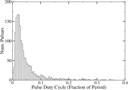
Figure 3: A histogram of the FWHM of currently known pulsars in units of fraction of duty cycle.

The angular width $\Delta\alpha$ of the pulsar emission is a crucial parameter in the probability of observation of deflected beams. Figure 3 shows a histogram, for currently known pulsars, of the FWHM of the pulse as a fraction of the pulse duty cycle. The mean of this distribution is 4.6%, so for probability calculations in this paper we will use a duty cycle of 5%, and therefore a value of 9^∘ for $\Delta\alpha$.

Of particular importance is the fact that a strongly bent beam will generally be reduced in intensity in comparison with a directly observed beam; thus our detection probabilities must account for the reduced brightness of the source. In terms of the bending function $F$ of Paper I, the “amplification” factor (generally less than unity) for intensity is given by

$${\frac{I}{I_{0}}}=\frac{\sin\phi_{\rm in}}{\sin\left(F\right)\,({dF}/{d\phi_{\rm in}})}\,.$$ (3)

As a step in understanding how much reduction can be allowed if a pulsar beam is to be observed, we use the radio luminosity at 1.4 GHz for all pulsars for which this quantity has been calculated in the Australia Telescope National Facility ATNF Pulsar Catalog (2010). We assume that the population of pulsars at the Galactic center has the same distribution of luminosities as these known pulsars. In that case, the distribution of pulsar flux densities $S$, observed at the Earth, would be that shown in Fig. 4.

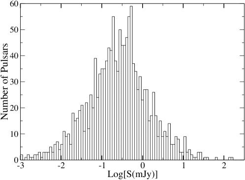
Figure 4: The distribution of pulsar L-band flux density $S$ that would be seen on Earth if all cataloged pulsars were located at the center of the Galaxy.

The minimum flux detectable at a telescope can be estimated with the following equation from  Lorimer & Kramer (2004) (hereafter LK):

$$S_{\rm min}=\frac{({\rm SNR}_{\rm min})\beta_{0}S_{\rm sys}}{\sqrt{n_{p}t_{obs}\Delta f}}\sqrt{\frac{W}{P-W}\;}\,.$$ (4)

Here $W$ and $P$ are respectively the pulsar pulse width and period. From our assumption that $W/P$ is 5% we get $\sqrt{W/(P-W)\;}=0.23$. The parameter $\beta_{0}$ is a correction factor for imperfections in data collection. Most current pulsar detection systems use a three-level correlarator with $\beta_{0}$ of 1.16 (see LK), and this is the value we shall use. For $n_{p}$, the number of polarizations recorded and summed in the detection process, we will use $n_{p}=2$ because typically two polarizations are summed during pulsar detection scans. ${\rm SNR}_{\rm min}$ is the minimum detectable signal-to-noise ratio required in a search; we will take this to be 5. For the time pointed at the source, $t_{obs}$, we will assume a 1 hour observing time. The bandwidth of the recorded data $\Delta f$ depends highly on the pulsar detection instruments used at a particular telescope. Bandwidths typically range from 100MHz to 800MHz. $S_{sys}$ is the system equivalent flux density which depends strongly on the collecting area of the telescope and the raw antenna sensitivity (see LK). The relevant characteristics of current existing radio telescopes and of possible future radio telescopes are detailed in Table 1.

Telescope Name	$S_{\rm sys}$(Jy)	$\Delta f({\rm MHz})$	$S_{\rm min}$(mJy)
Parkes	30	340	.022
GBT	10	800	.0048
FAST	1.5	800	.00072
SKA	.23	800	.00011

Table 1: Theoretical $S_{\rm min}$ values for two existing radio telescopes (Parkes, GBT) and two planned radio telescopes (FAST, SKA). The $S_{\rm sys}$ values for the existing radio telescopes are measured system equivalent flux densities and the $\Delta f$ values are for current recording instruments. The $S_{\rm sys}$ values for the two planned telescopes are theoretical values and the $\Delta f$ values were chosen to be the same as the best existing recording instruments.

3 Probability calculations

In this section we show how to calculate the probability that radiation from a single pulsar is detectable by a telescope on Earth, after having passed through the strong-field region of the black hole. This calculation naturally breaks down into two parts: determining what orientations of the pulsar and black hole produce strongly-bent beams, and determining where the Earth must be positioned relative to the system in order to detect those beams.

In Paper II it was shown that for any relative position of pulsar, black hole, and Earth, there are a set of directions, called “keyholes,” in which a photon could be emitted from the pulsar, pass around the black hole, and arrive at the Earth. These keyholes are typically within a few Schwarzschild radii of the black hole, so when the pulsar is far (many Schwarzschild radii) from the black hole, we can treat the keyhole as co-located with the black hole: that is, the pulsar beam must sweep across the black hole. The first part of the probability calculation is to determine for what fraction of the pulsar’s orbit it is in a position to illuminate the black hole with its beam.

We view the system from the perspective of the pulsar, so that the black hole traverses the sky of the pulsar along a great circle corresponding to the orbital plane. (This great circle in the pulsar sky does not imply that the pulsar-SMBH distance is constant.) Meanwhile, the pulsar spins about its rotation axis, and emits radiation in a cone offset from that axis: once per pulsar rotation the cone sweeps out an annulus in the sky of the pulsar. This is illustrated in Fig. 5, where $\alpha_{0}$, $\Delta\alpha$ and $\lambda$ have the meaning described in Sec. 2 and pictured in Fig. 2.

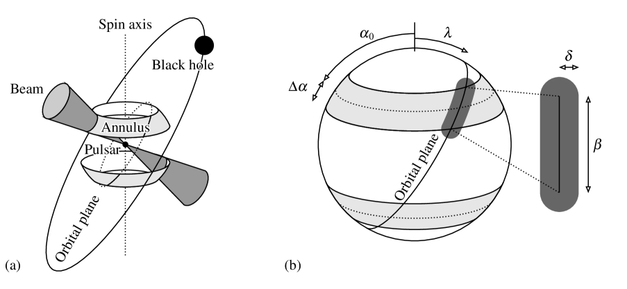
Figure 5: The geometry of a pulsar-black hole system as seen from the pulsar’s reference frame. Panel (a) shows how the pulsar beam sweeps out an annular region in the pulsar’s sky, which may intersect with the orbital plane of the pulsar-black hole system. Panel (b) shows the pulsar sky and labels the angles describing the orientation: $\lambda$ is the angle between the spin axis and orbital plane, $\alpha_{0}$ the angle between the spin axis and the center of the illuminated annulus (or beam), and $\Delta\alpha$ is the half-width of the annulus (or beam). The zoom on the right shows the region in the pulsar’s sky in which the Earth can lie if the photons reaching the Earth from the strong-field regime are to be bent by no more than an angle $\delta$.

With Fig. 5(b) we introduce the angle $\beta$, the total arc length (if any) over which the annulus intersects the orbital plane. When calculating $\beta$, it is useful to focus on one hemisphere at a time and to label the two edges of the pulsar’s radiation cone. We will define these two edges as $\alpha_{1}=\alpha_{0}-\Delta\alpha$ and $\alpha_{2}=\alpha_{0}+\Delta\alpha$. We break the calculation of $\beta$ into three cases, with one case having two subcases. The first case is that in which the orbital plane of the system is never illuminated by the pulsar’s radiation, $\alpha_{2}<\lambda$, as shown in Fig. 6. In this case, the value of $\beta$ is trivially zero.

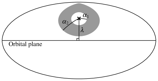
Figure 6: Schematic of the pulsar sky for case 1, in which the orbital plane does not intersect the annulus.

The second case is the case in which the orbital plane passes between the outer and inner edges of the annulus: $\alpha_{1}\leq\lambda<\alpha_{2}$. This case has two subcases. In the first subcase, that for $\alpha_{2}>\pi/2$, the entire orbital plane is illuminated by the pulsar, as shown in Fig. 7(a), The value of $\beta$ in this case is the entire range $\pi$ that lies in that hemisphere of the pulsar’s sky. (Remember that we are assuming symmetric emission about the pulsar’s rotational plane, so that the two beams together illuminate the full $2\pi$ range of the orbital plane.) The second subcase, when $\alpha_{2}\leq\pi/2$, has the outer edge of the annulus intersecting the orbital plane twice, as shown in Figure 7(b). In this case, $\beta$ can be found from the spherical triangle version of Pythagoras’s theorem, applied to the triangle with hypotenuse $\alpha_{2}$ and sides $\lambda$ and $\beta/2$: $\cos\alpha_{2}=\cos\lambda\cos\beta/2$, whence $\beta=2\arccos(\cos\alpha_{2}/\cos\lambda)$.

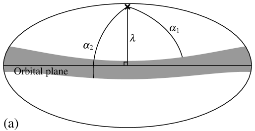
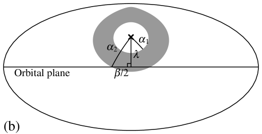
Figure 7: Schematic of pulsar sky for case 2, in which the orbital plane passes between the outer and inner edges of the annulus. In panel (a), the orbital plane is entirely contained within the annulus. In panel (b), it crosses the outer edge of the annulus at two points symmetric about the meridian containing the spin axis.

The final case has both the outer and inner edges of the annulus crossing the orbital plane, $\alpha_{1}>\lambda$, as illustrated in Figure 8. The calculation proceeds as in the previous case, but considers only the range of $\beta$ between the triangles with hypotenuses $\alpha_{2}$ and $\alpha_{1}$: $\beta=2\arccos(\cos\alpha_{2}/\cos\lambda)-2\arccos(\cos\alpha_{1}/\cos\lambda)$.

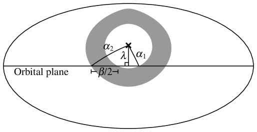
Figure 8: Schematic of pulsar sky for case 3, in which orbital plane intesects both the inner and outer edges of the annulus.

The cases and calculations for $\beta$ are summarized in the following:

$$\begin{array}[]{|c|cc|l|}\hline\cr\mbox{Case}&\vrule\lx@intercol\hfil\mbox{Condition}\hfil\lx@intercol\vrule\lx@intercol&~{}\mbox{$\beta$ Calculation}\\ \hline\cr&&&\\[-8.61108pt] \begin{array}[]{l}1{}\end{array}&\alpha_{2}\leq\lambda&&\begin{array}[]{l}\beta=0\end{array}\\[4.30554pt] \begin{array}[]{l}\mbox{2a}\\[4.30554pt] \mbox{2b}\end{array}&\alpha_{1}\leq\lambda<\alpha_{2}&\left\{\begin{array}[]{c}\alpha_{2}\geq\pi/2\\[4.30554pt] \alpha_{2}<\pi/2\end{array}\right.&\begin{array}[]{l}\beta=\pi\\[4.30554pt] \beta=2\arccos\left(\frac{\cos\alpha_{2}}{\cos\lambda}\right)\end{array}\\[12.91663pt] \begin{array}[]{l}3{}\end{array}&\lambda<\alpha_{1}&&\begin{array}[]{l}\beta=2\arccos\left(\frac{\cos\alpha_{2}}{\cos\lambda}\right)-2\arccos\left(\frac{\cos\alpha_{1}}{\cos\lambda}\right)\end{array}\\[4.30554pt] \hline\cr\end{array}$$

The second part of the probability calculation is to determine how often the Earth will be in a position to detect strongly-bent beams from the system. This imposes geometric limitations to ensure that we are considering beams that are significantly deflected by the black hole, but that are not deflected so strongly that they are attenuated to a flux too low to be detected. These constraints turn out to place limits on the acceptable range of $\phi_{\rm out}$.

The determination of that range is shown in Fig. 9 for the case $r_{0}=100M$. That figure shows the dramatic amplification at $\phi_{\rm out}=\pi$, corresponding to strong lensing. For $\phi_{\rm out}$ slightly less than $\pi$, the attenuation factor is unity, and the bending is not significant. There is bending for $\phi_{\rm out}<\pi$, but the range of $\phi_{\rm out}$ for which there is significant bending is small. Moreover, this range is even smaller than in Fig. 9 for the larger, more relevant values of $r_{0}/M$. As a convenient approximation, therefore, we will consider “strong bending” only for $\phi_{\rm out}\geq\pi$. The figure shows that as $\phi_{\rm out}$ incresses beyond $\pi$ the attenuation becomes greater and greater.

Our approach will be to specify a radius of emission $r_{0}$ and a minimum acceptable value of $I/I_{0}$. From a calculation like that shown in Fig. 9 we then find the value of the angle $\delta$, the value of $\phi_{\rm out}-\pi$ at which the attenuation is that of the minimum acceptable value of $I/I_{0}$. This value of $\delta$ determines the range of directions in which the Earth must located if an Earth telescope is to detect the beam: the Earth must lie no more than an angle $\delta$ from the pulsar-black hole axis.

The corresponding region on the pulsar sky is illustrated in Fig. 5(b). Since $\delta$ is typically very small, we can express this area using a flat-space approximation: $2\beta\delta+\pi\delta^{2}$. The probability that observers on Earth can detect strongly-bent beams from a given pulsar is given by the size of this area over the angular area of one hemisphere (again, we assume symmetry across the rotation plane of the pulsar):

$$P_{1}\;\;=\;\;\frac{2\beta\delta+\pi\delta^{2}}{2\pi}\,.$$ (5)

This of course assumes nonzero $\beta$: if $\beta=0$, the black hole is not illuminated by the pulsar, and there are no strongly-bent beams, so $P_{1}=0$. Note that $\beta$ is a function of the underlying parameters $\lambda$, $\alpha_{0}$, and $\Delta\alpha$, and note that $\delta$ is a function of the underlying parameters $r_{0}/M$ and $I_{\mathrm{min}}/I_{0}$.

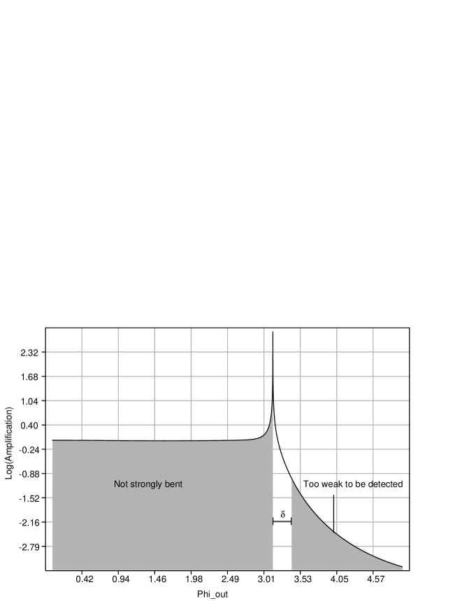
Figure 9: The intensity ratio ${I}/{I_{0}}$ as a function of $\phi_{\rm out}$, for $r_{0}=100M$. The shaded regions show the ranges of $\phi_{\rm out}$, that are not of interest either because the pulsar beam is too weakly deflected or because it is too strongly attenuated.

4 Results

Now that we have shown how to calculate the probability of Earth detection for a particular pulsar, we will describe how we estimated the number of pulsars that would be detected given assumptions about the distributions of pulsar characteristics. We ran Monte Carlo simulations that selected $\lambda$ from a uniform distribution of $\cos{\lambda}$, so that the direction of the pulsar spin axis was uniformly distributed over the sky; similary $\alpha_{0}$ was chosen from a uniform distribution of $\cos{\alpha_{0}}$. Then a value for the pulsar’s flux, $S$, was chosen from the distribution shown in Fig. 4. Lastly, a value of $r_{0}/M$ was chosen from the distribution in Eq. (1); we cut this distribution off at $r_{0}/M=400,000$ since pulsars beyond that point contribute little to the total probability (see below).

The simulations took the pulsar parameters ($r_{0}$, $S$) chosen by the Monte Carlo method. From these a determination was made of the minimum value of $I/I_{0}$ (equivalently $S_{\rm min}/S$) that can be detected for those pulsar parameters. From $I/I_{0}$ and $r_{0}$, the value of $\delta$ was determined. The value of $\beta$ was detemined through the calculations described in the previous section applied to the values of $\lambda$ and $\alpha_{0}$ chosen by the Monte Carlo method. The justification for using $\Delta\alpha=9^{\circ}$ has been explained in Sec. 2. $P_{1}$ was then calculated with Eq. 5. This gives us the probability that a single pulsar’s beam will explore the black hole’s strong gravitational field and still be detectable once it reaches the Earth. Monte Carlo simulations were repeated to insure that results were consistent to better than 1%. We then multiplied our result by the total number of pulsars out to $r_{0}=400,000$, according to the Pfahl and Loeb distribution of Eq. (1). The result is the total number of pulsars ($P_{\rm tot}$) that will, at some point in their orbit about the central SMBH, both illuminate the strong gravitational field and be detectable at Earth. Table 2 gives this number for the four telescopes considered in Sec. 2.

Telescope Name	$S_{\rm sys}$(Jy)	$P_{\rm tot}$
Parkes	.022	8.75776
GBT	.0048	15.8075
FAST	.00072	111.677
SKA	.00011	207.021

Table 2: $S_{\rm min}$ and $P_{\rm tot}$ values for two existing radio telescopes (Parkes, GBT) and two planned radio telescopes (FAST, SKA).

The number of pulsars that are observable at some point in their orbit is not directly relevant if the orbital time is much larger than the duration of an observing program. For that reason we introduce a more useful number, the “observability,” $P_{\rm obs}$, to describe the probability of observing a given pulsar in a limited-time observing program. In order to calculate this number, we ran the Monte Carlo simulations with a specified observational program duration ($L$). Once $P_{1}$ was calculated, we then compared the pulsar’s orbital period ($T$) to $L$. If $T$ was less than or equal to $L$, then $P_{\rm obs}$ was taken to be $P_{1}$. If $T$ was greater than $L$, then $P_{1}$ was replaced by

$$P_{\rm obs}=\frac{P_{1}\times{L}}{T}\,,$$ (6)

and the result was multiplied by the total number of pulsars. Figure 10 shows the results of the Monte Carlo simulations for observational program durations ranging from one year to seven years.

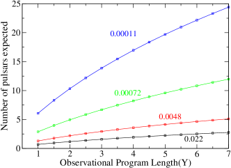
Figure 10: Expected number of pulsars observed as a function of observational program duration. Curves are labeled with the values of $S_{\rm min}$, in mJy, assumed in the computations.

Figure 11 shows the variation in the number of pulsars detected, for $S_{\rm min}=0.022$ mJY, as the cutoff radius is changed, and justifies our use of the cutoff at $r_{0}/M=4\times 10^{5}$.

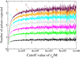
Figure 11: The number of pulsars expected, for $S_{\rm min}=0.022$ mJy, as a function of the cutoff $r_{0}/M$ for the distribution in Eq. (1). Each curve is labeled with the number of years assumed for the search.

5 Observing Programs and Strategies

A natural first question about observing strongly deflected beams is “how will we know that they are strongly deflected?” The answer starts with the fact that the angle through which the beam is “strongly” deflected is not large. For our paradigmatic case, $r_{0}=10^{4}M$, the bending is approximately 0.036 rad. For larger $r_{0}$ the deflection, for a given $S_{\rm min}$, is even smaller.

Since the “strong” deflection is small, we will receive a deflected beam only when the emitting pulsar, the SMBH and the Earth are almost on a straight line. Since pulsar beam widths are large compared to the deflection, this means that if the Earth receives the deflected beam, it will also receive the direct beam. The geometry of the direct and deflected beams is shown in Fig. 12, where we see that the angle, at reception, of the direct and deflected beams is not of order $r_{0}$ divided by the Earth-SMBH distance (8 kpc), but rather is of order of that number multiplied by the deflection angle. The result, an angle of order $10^{-8}$ radians, is less than the resolution of radio telescopes. We conclude that any monitoring of the innermost region of Sgr A^∗ for a deflected beam, will also monitor for a direct beam.

The criterion for the detection of a strongly deflected beam will be that it is one of a pair of pulses detected with very similar pulse periods, differing only due to a phase modulation caused by variations in the propagation times along the two paths: the two sets of pulses will differ in pulse period by a fractional amount of order the pulsar velocity divided by $c$. (See Papers I and II for more detail on phase effects and intensity effects of deflection.) If a deflected beam is detected we therefore assume that it will be relatively simple to identify it as deflected.

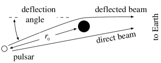
Figure 12: The geometry of the observation of direct and deflected beams.

If the Pfahl and Loeb distribution of Eq. (1) is approximately valid, the results of the previous section, especially Fig. 10, suggest that there is a very good chance of observing a strongly deflected pulsar beam with an observing program of 3-5 years, using existing telescopes. Monitoring of Sgr A^∗, of course, will face the problem of dispersion by the plasma density in the Galactic center. Assuming dispersion measures in excess of $1000\,\mathrm{pc}/\mathrm{cm}^{3}$, searches would have to be conducted in S-band (2–4 GHz) or higher frequencies in order to resolve pulses, rather than the more conventional L-band.

We note that the pulsar fluxes and current telescope sensitivities were computed for the L band, since that is where most pulsar luminosities have been measured. Relative sensitivities in the S band may be somewhat lower. However, we note that the baseline value of $S_{\rm min}=0.022$ mJy for the Parkes telescope is very conservative in view of the sensitivities that will soon be available. See Table 1, and the corresponding estimates of detectable pulsars in Fig. 10. Even with the current estimated senstitivity of Parkes there is a good chance of detecting strongly-bent pulsar beams in a 2–3 year observing program; with more sensitive telescopes such as GBT or FAST (under development), the number could rise to several pulsars. Longer observing times increase the number of detectable pulsars by allowing long-period pulsars more time to come into alignment.

An appropriate multiyear observing program can be carried out “in background” at a telescope. Observations must be made sufficiently frequently not to miss the relatively short epoch during which the pulsar/SMBH/Earth alignment leads to a strongly deflected beam meeting the $I/I_{0}$ criterion. That epoch is of order of the orbital time multiplied by the ratio $\delta/(2\pi)$. For our prototypical choice $r_{0}=10^{4}\,M$, this epoch is on the order of a week. Searches for deflected beams in Sgr A^∗, therefore, would have to be made every other day. The observing session would be of a duration of that used for any other pulsar search, on the order of 1 hour. (Longer observations might be considered, in view of the effect shown in Eq. (4) of $t_{obs}$ on $S_{\rm min}$, and hence on the $I/I_{0}$ cutoff.

An important question to ask is why we do not yet have evidence of the assumed large population of pulsars in Sgr A^∗. This can be explained by the lack of any concerted effort to search the Galactic center for pulsars, and the need for S band searches with large dispersion corrections. In addition the Galactic Center is out of view for the Arecibo telescope, and in a portion of the sky with reduced sensitivity for GBT. Currently, Parkes is the largest telescope with a clear view of the Galactic Center; the FAST telescope will substantially increase our sensitivity to the Galactic Center.

It should be noted that, at least to some extent, monitoring the Galactic center for strongly deflected beam would constitute a more general search for pulsars in that region. The possibility of detecting deflected beams and making measurements of the parameters of the SMBH provides added scientific motivation for such a survey.

6 Conclusions

Our estimates suggest that a multi-year program that monitors Sgr A^∗ with radio observations for one hour every other day has a reasonable probability of detecting pulsar beams that have been strongly deflected by our Galaxy’s SMBH. With instruments coming in the near future, in particular, FAST and SKA, the probability should become high enough so that a three year observational program either detects a strongly deflected beam, or that the failure to make such a detection puts useful limits on the density of pulsars in the Galactic Center.

Our estimates in this paper constitute a first step in the study of probabilities of detection of a strongly deflected beam. The intention was to establish whether the probabilities are so small that observations are out of the question, or so large that current observations rule out models, like that of Pfahl & Loeb (2004), with a significant density of pulsars in Sgr A^∗. The estimates in this paper establish neither extreme: a concerted observing program with the best current telescopes would optimistically detect only a few such pulsars. This provides motivation for such a program, and also for further study of the problem of pulsar beam deflection by SMBHs.

Such an improved study would have to include effects of spin of the SMBH, and of eccentricity of orbits. While our approach of using averages and simple assumptions was appropriate to the purpose of this paper, effects due to SMBH spin, and high eccentricity, could increase the parameter space of pulsar configurations whose beams can reach the Earth. Such work is now underway.

The most exciting result of these preliminary estimates is their indication that we are potentially on the verge of detecting a new phenomenon: pulsar beams that have passed through the strong field region of the SMBH at the center of our Galaxy, beams that can bring us information about the properties of the SMBH and its surrounding spacetime might be inaccessible in any other way.

We gratefully acknowledge support by the National Science Foundation under grants AST0545837, PHY0554367 and HRD0734800. We also thank the Center for Gravitational Wave Astronomy at the University of Texas at Brownsville.

7 Appendix

We are primarily interested in values of $\phi_{\rm in}$ that are only slightly smaller than $\pi$. In this case the photon path starting at some very large radius will penetrate to small radii, and almost all the bending will take place at small radii. We can then find the bending for emission from the very large radius, say $R_{0}=10,000\,M$, by considering the bending only interior to a smaller large radius, say $r_{0}=100\,M$. In effect, we are considering the large radius region from $R_{\rm o}$ to $r_{\rm o}$ to be flat space. From the the curve $F(\phi_{\rm in};r)$ for $r_{0}=100\,M$, therefore, we can infer the curve for $R_{0}=10,000\,M$, and for all larger radii (provided, of course, that $\phi_{\rm in}$ is near $\pi$ so that both $R_{\rm o}$ and $r_{\rm o}$ are much larger than the radii at which the bending occurs).

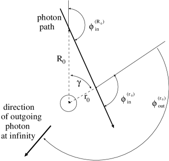
Figure 13: The flat spacetime propagation from large radius to very large radius. Angles $\phi_{\rm in}$ for the large, and the very large emission radius are distinguished with the superscripts $(r_{0})$ and $(R_{0})$, respectively.

To find the $\phi_{\rm out}^{\rm(R_{0})}$ for a photon emitted at a very large $R_{0}$, we choose the smaller $r_{0}$ along the future path of the photon to be a radius for which we know the curve $\phi_{\rm out}^{\rm(r_{0})}=F(\phi_{\rm in}^{\rm(r_{0})};r_{0})$. Here superscripts $(r_{0})$ and $(R_{0})$ distinguish the angles associated with the two radii. The Euclidean geometry relating $\phi_{\rm in}^{\rm(r_{0})}$ and $\phi_{\rm in}^{\rm(R_{0})}$ is given by the law of sines to be

$$\phi_{\rm in}^{\rm({r_{\rm 0}})}=\sin^{-1}\!\left([R_{0}/r_{0}]\sin{\phi_{\rm in}^{\rm({R}_{\rm 0})}}\right)\,,$$ (7)

and we choose the branch of $\sin^{-1}$ so that $\phi_{\rm in}^{\rm({r_{\rm 0}})}>\pi/2$.

We next notice that $\phi_{\rm out}$ for the photon starting at $r_{0}$ is less than $\phi_{\rm out}$ for that same photon world line considered to start at $R_{0}$, in flat space, according to

$$\phi_{\rm out}^{(\rm{R}_{0})}=\phi_{\rm out}^{(\rm{r}_{0})}+\gamma\,.$$ (8)

With $\gamma$ evaluated in terms of the ingoing angles, this becomes

$$\phi_{\rm out}^{\rm({R}_{0})}=\phi_{\rm out}^{\rm({r}_{0})}+\phi_{\rm in}^{\rm({R}_{0})}-\phi_{\rm in}^{\rm({r}_{0})}\,.$$ (9)

From a combination of Eqs. (7) and (9), written in terms of the function $F(\phi;r)$, the full expression can be given as:

$$F(\phi;R_{0})\;\;=\;\;\phi+F\left[\sin^{-1}\!\left(\mbox{$\frac{R_{0}}{r_{0}}$}\sin\phi\right);r_{0}\right]-\sin^{-1}\!\left(\mbox{$\frac{R_{0}}{r_{0}}$}\sin\phi\right)$$ (10)

Thus, knowing the $F$ function for any (sufficiently large) $r_{0}$, we can evaluate it for any larger $R_{0}$, and thus determine the maximum deflection angle $\delta$ via Eq. (3). Figure 14 shows our reference bending function for a radius $r_{0}=100M$.

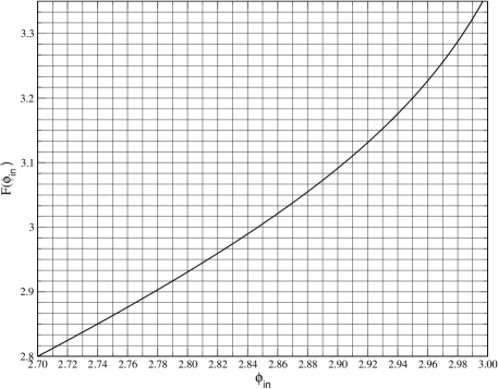
Figure 14: The bending function $\phi_{\rm out}=F(\phi_{\rm in})$ for bending angles near $\pi$, for an initial radius $r_{0}=100M$.

References

- ATNF Pulsar Catalog (2010) ATNF Pulsar Catalog. 2010, http://www.atnf.csiro.au/research/pulsar/psrcat
- Deegan & Nayakshin (2007) Deegan, P., & Nayakshin, S. 2007, MNRAS, 377, 897
- Eisenhauer et al. (2005) Eisenhauer, F., Genzel, R., Alexander, T., Abuter, R., Paumard, T., Ott, T., Gilbert, A., Gillessen, S., Horrobin, M., Trippe, S., Bonnet, H., Dumas, C., Hubin, N., Kaufer, A., Kissler-Patig, M., Monnet, G., Ströbele, S., Szeifert, T., Eckart, A., Schödel, R., & Zucker, S. 2005, ApJ, 628, 246
- Freitag et al. (2006) Freitag, M., Amaro-Seoane, P., & Kalogera, V. 2006, Journal of Physics Conference Series, 54, 252
- Genzel et al. (2003) Genzel, R., Schödel, R., Ott, T., Eckart, A., Alexander, T., Lacombe, F., Rouan, D., & Aschenbach, B. 2003, Nature, 425, 934
- Ghez et al. (2005) Ghez, A. M., Salim, S., Hornstein, S. D., Tanner, A., Lu, J. R., Morris, M., Becklin, E. E., & Duchêne, G. 2005, ApJ, 620, 744
- Hopman & Alexander (2006) Hopman, C., & Alexander, T. 2006, Journal of Physics Conference Series, 54, 321
- Lorimer & Kramer (2004) Lorimer, D. R., & Kramer, M. 2004, Handbook of Pulsar Astronomy, ed. Lorimer, D. R. & Kramer, M., (LK)
- Maness et al. (2007) Maness, H., Martins, F., Trippe, S., Genzel, R., Graham, J. R., Sheehy, C., Salaris, M., Gillessen, S., Alexander, T., Paumard, T., Ott, T., Abuter, R., & Eisenhauer, F. 2007, ApJ, 669, 1024
- Melia et al. (2001) Melia, F., Bromley, B. C., Liu, S., & Walker, C. K. 2001, ApJ, 554, L37
- Muno et al. (2005) Muno, M. P., Pfahl, E., Baganoff, F. K., Brandt, W. N., Ghez, A., Lu, J., & Morris, M. R. 2005, ApJ, 622, L113
- Nayakshin & Sunyaev (2005) Nayakshin, S., & Sunyaev, R. 2005, MNRAS, 364, L23
- Pfahl & Loeb (2004) Pfahl, E., & Loeb, A. 2004, ApJ, 615, 253
- Wang et al. (2009a) Wang, Y., Creighton, T., Price, R. H., & Jenet, F. A. 2009a, ApJ, 705, 1252, (Paper II)
- Wang et al. (2009b) Wang, Y., Jenet, F. A., Creighton, T., & Price, R. H. 2009b, ApJ, 697, 237, (Paper I)