Electric signature of magnetic domain-wall dynamics

Abstract

Current-induced domain-wall dynamics is studied in a thin ferromagnetic nanowire. The domain-wall dynamics is described by simple equations with four parameters. We propose a procedure to unambiguously determine these parameters by all-electric measurements of the time-dependent voltage induced by the domain-wall motion. We provide an analytical expression for the time variation of this voltage. Furthermore, we show that the measurement of the proposed effects is within reach of current experimental techniques.

Introduction. Recently, applications for future memory and logic devices, as well as important fundamental physics questions, have stimulated a number of experimental Yamaguchi04 ; Thomas2006 ; Thomas2007 ; Meier07 ; Rhensius10 ; IlgazPRL10 ; Krivorotov10 ; BeachPRL09 and theoretical Beach:review08 ; YanAPL10 ; YanEPL10 studies of the current-driven domain wall (DW) dynamics in ferromagnetic nanowires. It has been shown that DWs can be moved by a current either parallel Yamaguchi04 ; Thomas2006 ; Thomas2007 ; Meier07 ; Rhensius10 ; IlgazPRL10 or perpendicular to the wire. Krivorotov10 ; YanAPL10 ; YanEPL10 In some of the experiments short current pulses were employed to depin a DW from pinning sites. Thomas2006 ; Thomas2007 ; IlgazPRL10 Furthermore, the topological electromotive force induced by DW dynamics in a vortex DW has been studied both experimentally and theoretically. BeachPRL09 ; Yang2010

A conventional experimental method to study the DW dynamics in nanowires is to measure the average DW velocity using Kerr polarimetry, Beach05 x-ray microscopy, Meier07 or electron microscopy. Rhensius10 ; Klaui:images05 These types of experiments require a complicated setup which is separate from the one needed for the DW manipulation. This situation is neither ideal for studies of DW dynamics nor for further technological advances.

In this Letter we propose a way to use the same experimental setup for both current DW manipulation and simultaneous measurements of DW dynamics. Our main results are that the time-dependent voltage induced by the DW motion Tserkovnyak2008 ; Duine09 can be used to fully and comprehensively determine the effective parameters of the DW dynamics. This proposal follows from the fundamental properties of the current-induced DW motion, namely: (i) Applied DC current (above critical value) produces voltage with AC components. (ii) Applied AC current induces phase shifted AC voltage. The magnitude of the proposed effects is calculated to be within current experimental resolution.

Similar techniques have already shown promise in magnetic field driven DW systems. Singh10 This method should make it more feasible to utilize DW dynamics for device applications. Furthermore, the proposed systematic approach can be used to compare the extracted phenomenological parameters of the DW dynamics for a system described by arbitrary underlying Hamiltonian to those of microscopic theories.

Model. The dynamics of the magnetization $\mathbf{S}$ in a quasi-one-dimensional wire is described by Landau-Lifshitz-Gilbert (LLG) equation with current $j$, Zhang04 ; Thiaville05

$$\dot{\mathbf{S}}=-\mathbf{S}\times\mathbf{H}_{e}-j\partial_{z}\mathbf{S}+\beta j\mathbf{S}\times\partial_{z}\mathbf{S}+\alpha\mathbf{S}\times\dot{\mathbf{S}},$$ (1)

where $\mathbf{H}_{e}=-\delta\mathcal{H}/\delta\mathbf{S}$ is the effective magnetic field given by the Hamiltonian $\mathcal{H}$ of the system, $\mathbf{S}=\mathbf{M}/|M|$ is a unit magnetization vector, $\alpha$ is the Gilbert damping constant, $\beta$ is the non-adiabatic spin torque constant, $\partial_{z}\equiv\partial/\partial z$ where $\mathbf{\hat{z}}$ is along the wire, and the time is measured in units of the gyromagnetic ratio $\gamma_{0}=g|e|/(2mc)$. DWs in a ferromagnetic wire can be modeled by a spin Hamiltonian $\mathcal{H}$ which contains exchange, spin-orbit, and dipolar interactions. In a thin wire, the latter can be approximated by two anisotropies: a strong anisotropy along the wire ($\lambda$) and a weak anisotropy transverse to it ($K$). In realistic systems $\alpha,\beta\ll 1$ and $K\ll\lambda$.

In a thin wire, a lowest-energy magnetization configuration (at $j=0$) is uniformly ordered along the $z$ or $-z$ direction. A static DW is the next low-energy configuration with the boundary conditions $S_{z}(\pm\infty)=\pm 1$ or $S_{z}(\pm\infty)=\mp 1$. DWs can be injected in the wire using different techniques. A sketch of a wire with a DW of width $\Delta$, determined by the Hamiltonian parameters, is depicted in Fig. 1.

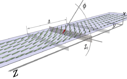
Figure 1: (Color online) A moving head-to-head domain wall of width $\Delta$. The DW is centered at $z_{0}$ and is tilted by an angle $\phi$.

For small enough applied currents, it can be shown that the DW in a thin wire is a rigid spin texture Klaui:images05 and its dynamics can be described in terms of only two collective coordinates. Tatara04 ; Tretiakov_DMI These coordinates correspond to the two softest modes of the DW motion: the DW position along the wire, $z_{0}$, and the rotation angle $\phi$ of the magnetization in the DW around the wire axis, see Fig. 1. It has been shown Tretiakov:losses ; Tretiakov_DMI that the equations of motion for the DW in a thin ferromagnetic wire are model independent and can very generally be written in the form

$$\dot{z}_{0}=Aj+B[j-j_{c}\sin(2\phi)],$$ (2)

$$\dot{\phi}=C[j-j_{c}\sin(2\phi)].$$ (3)

Here all current nonlinearities are neglected, since the large currents leading to observable nonlinear effects would burn the nanowire. For a dc current below the critical value $j_{c}$, i.e., $j<j_{c}$, Eq. (3) implies that the DW tilts from the transverse anisotropy plane by the angle that satisfies $\sin(2\phi)=j/j_{c}$ around the wire axis and then moves along the wire with a constant velocity $Aj$. For $j>j_{c}$, the DW constantly rotates while moving.

The coefficients $A$, $B$, $C$ and the critical current $j_{c}$ are the parameters that fully describe the DW dynamics. They can be calculated microscopically for certain toy models, Tretiakov_DMI but in general they vary for different wires and depend on the temperature and nanofabrication details. Therefore, in this Letter we propose a way to determine these coefficients by model-independent measurements of an induced ac voltage directly from an experiment suitable for all-electric DW manipulation. As we show below, this ac voltage can be induced by applied dc currents and by certain time-dependent current pulses with parameters similar to those achieved in recent experiments. KlauiPRL05 ; KlauiAPL10

Microscopically the dynamics parameters can be obtained in the following way. The energy of a static DW, $E_{0}(z_{0},\phi)=\int\mathcal{H}[\mathbf{S}_{0}(z,z_{0},\phi)]dz$, where $\mathbf{S}_{0}$ is a solution of a static LLG with $K=0$, in general depends on both $z_{0}$ and $\phi$. However, assuming that the wire is translationally invariant (pinning can be neglected), $E_{0}$ would not depend on the DW position $z_{0}$ and therefore $\partial_{z_{0}}E_{0}=0$. The only contribution to $E_{0}$ that depends on the angle $\phi$ comes from the small anisotropy in the transverse plane, $E_{0}(\phi)=-\kappa\cos(2\phi)$. Tretiakov_DMI This allows us to find the coefficients in Eqs. (2) and (3) in terms of the parameters of the LLG (1). Tretiakov_DMI ; future Up to first order in $\alpha$ and $\beta$ they are

$$A=\frac{{\tilde{\beta}}}{{\tilde{\alpha}}},\qquad B=\frac{{\tilde{\alpha}}-{\tilde{\beta}}}{{\tilde{\alpha}}}(1+{\tilde{\alpha}}a_{z\phi}),$$ (4)

$$C=({\tilde{\alpha}}-{\tilde{\beta}})a_{zz},\qquad j_{c}=\frac{{\tilde{\alpha}}}{{\tilde{\alpha}}-{\tilde{\beta}}}\kappa,$$ (5)

where ${\tilde{\alpha}}=\alpha\mathcal{D}$, ${\tilde{\beta}}=\beta\mathcal{D}$, $\mathcal{D}=\sqrt{a_{zz}a_{\phi\phi}-a_{z\phi}^{2}}$, $a_{zz}=\frac{1}{2}\int dz(\partial_{z}\mathbf{S}_{0})^{2}$, $a_{\phi\phi}=\frac{1}{2}\int dz(\partial_{\phi}\mathbf{S}_{0})^{2}$, and $a_{z\phi}=\frac{1}{2}\int dz\partial_{z}\mathbf{S}_{0}\cdot\partial_{\phi}\mathbf{S}_{0}$. Equations (4) and (5) are consistent with the expressions for $A$, $B$, $C$, and $j_{c}$ found in Ref. Tretiakov_DMI, .

We now outline the method to find $A$, $B$, $C$, and $j_{c}$ directly from all-electric measurements. It is based on measuring the ac voltage $V$ induced by a moving DW. To find $V$ one has to know the time evolution of the total energy (per unit area of the wire’s cross-section) in the system,

$$\dot{E} = \int dz\frac{\delta\mathcal{H}}{\delta\mathbf{S}}\cdot\dot{\mathbf{S}}(z).$$ (6)

In general, DW energy has two contributions: the power supplied by an electric current and a negative contribution due to dissipation in the wire. Using the general solution of the LLG, Eq. (1), one can obtain the derivative of the energy as Tretiakov_DMI ; future

$$\dot{E}=2[\beta a_{zz}\dot{z}_{0}+(1-\beta a_{z\phi})\dot{\phi}]j-\alpha\int dz\dot{\mathbf{S}}_{0}^{2}.$$ (7)

The last term on the right-hand side of Eq. (7) describes the dissipation and is therefore always nonpositive. Meanwhile, the first term is proportional to the current density $j$ and gives the power $Vj$ supplied by the current. With the help of Eqs. (4)–(5) and adopting the approximation $\mathcal{D}\simeq 1$ of Ref. Tretiakov_DMI, we obtain the expression for the induced DW voltage ,

$$V=\frac{A^{2}C}{B}j+C(1+A)[j-j_{c}\sin(2\phi)].$$ (8)

Note that Eq. (8) gives the contribution to the voltage due to DW motion. This contribution is in addition to the usual Ohmic one. The voltage $V$ in Eq. (8) is measured in units of $Pg\mu_{B}/(e\gamma_{0})$ and the current density is measured in units $2eM/(Pg\mu_{B})$, where $P$ is the current polarization. We emphasize that unlike in the previously studied cases, BeachPRL09 ; Yang2010 this voltage is not caused by the motion of topological defects (vortices) transverse to the wire.

Measurement of coefficients $A$, $B$, $C$, and $j_{c}$. In order to find coefficients $A$, $B$, and $C$, we propose three independent measurements of the voltage induced by a moving DW. Although there are various factors affecting the nanowire resistance, the contributions from most of them are independent of DW motion and therefore give only a constant component of the resistance. To characterize the DW dynamics, one has to concentrate only on the resistance variations in time. Our estimates show that the amplitude of voltage oscillations due to DW motion is of the order of $10^{-7}$ V and therefore experimentally measurable.

Equation (8) implies that the voltage of the DW can give all the necessary information about DW dynamics. Namely, one can obtain $C$ by measuring the voltage changing with time and parameters $A$ and $B$ by measuring the amplitude of the voltage oscillations.

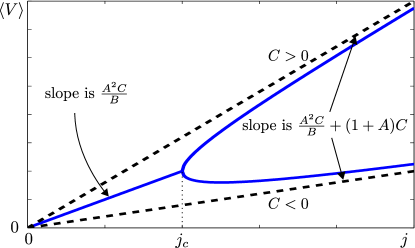
Figure 2: (Color online) Dependence of average voltage $\langle V\rangle$ on dc current $j$ for $C>0$ and $C<0$, respectively, see Eq. (8). The slope at $j<j_{c}$ gives $\frac{A^{2}C}{B}$, whereas at $j\gg j_{c}$ it gives $\frac{A^{2}C}{B}+(1+A)C$.

Slopes measurement. In Refs. Tretiakov:losses, ; Tretiakov:JAP, it was proposed to obtain $A$, $B$, and $j_{c}$ by measuring the drift velocity of the DW, $\langle\dot{z}_{0}\rangle$. It is important to note that Eq. (8) has the same form as Eq. (2). Thus, instead of measuring the drift velocity, which requires a more complicated experimental setup, we propose to perform all-electric measurements. Namely, to measure the average voltage of DW, $\langle V\rangle$, as a function of dc current. From Eq. (8) one can see that $\langle V\rangle=\frac{A^{2}C}{B}j$ for $j<j_{c}$, whereas $\langle V\rangle=\frac{A^{2}C}{B}j+(1+A)C\sqrt{j^{2}-j_{c}^{2}}$ for $j>j_{c}$, see Fig. 2. The critical current is determined by the end of the region linear in $j$ for small currents. The measurement of slope $k_{1}$ at $j<j_{c}$, and slope $k_{2}$ at $j\gg j_{c}$ gives the two independent quantities:

$$k_{1}=\frac{A^{2}C}{B},\qquad k_{2}-k_{1}=(1+A)C.$$ (9)

Instead of measuring voltage average for dc current, one can apply a linearly increasing time-dependent current $j(t)=qt$ below the critical value $j_{c}$. At sufficiently small $q$ the voltage will also be linear in time, $V(t)\approx\frac{A^{2}C}{B}qt$. By measuring this voltage one can find

$$\frac{V(t)}{j(t)}=\frac{A^{2}C}{B}.$$ (10)

Once $C$ is determined, Eqs. (9) give $A$ and $B$. The drawback of this measurement is that it might be hard to disentangle $k_{1}$ and $k_{2}$ from the Ohmic contribution. However $k_{2}-k_{1}$ is free from the Ohmic resistance of the wire.

In order to find $C$, the most intuitive approach is to input a dc current slightly above $j_{c}$. Then the voltage induced by the moving DW will oscillate with the period of the double angle $\phi$, see the insets of Fig. 3. The half-width of the peak (dip) for $C>0$ ($C<0$) is given by $\arccos(j_{c}/j)/(|C|\sqrt{j^{2}-j_{c}^{2}})$. The measurement of the voltage oscillations period $T_{0}$ (which we estimate to be $\sim 10^{-7}$ – $10^{-6}$ s) determines $C$ at a given $j$:

$$|C|=\frac{1}{T_{0}}\int_{0}^{\pi}\frac{d\phi}{j-j_{c}\sin(2\phi)}=\frac{\pi}{T_{0}\sqrt{j^{2}-j_{c}^{2}}}.$$ (11)

For $j-j_{c}\ll j_{c}$, the period diverges but the half-width $\sim 1/(Cj_{c})$ stays finite. To obtain the period $T_{0}$, one can perform the Fourier transform of $V(t)$ to find the frequency $f_{0}=1/T_{0}$, see Fig. 3.

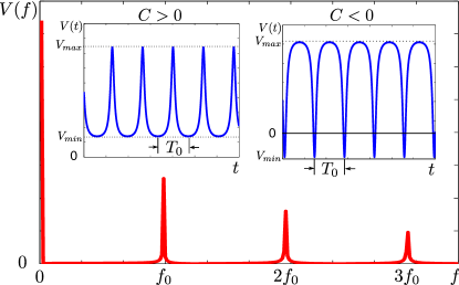
Figure 3: (Color online) Fourier transform of the voltage $V$ as a function of frequency $f$ at the dc current $1.1j_{c}$. The insets show $V$ as a function of time $t$ for $C>0$ given by $\alpha=0.02$ and $\beta=0.01$; and for $C<0$ given by $\alpha=0.01$ and $\beta=0.02$. The voltage period is $T_{0}=1/f_{0}$. In the inset for $C<0$, the voltage varies between $V_{max}=0.041j_{c}/\Delta$ and $V_{min}=-0.019j_{c}/\Delta$.

To determine coefficient $A$ in the same experiment, one can measure $\Delta V=V_{max}-V_{min}=2(1+A)|C|j_{c}$, see insets of Fig. 3. Then

$$A=\frac{\Delta V}{2|C|j_{c}}-1.$$ (12)

Note that $\Delta V=2(k_{2}-k_{1})j_{c}$ and therefore this experiment can also provide a crosscheck with the aforementioned measurement of the slopes.

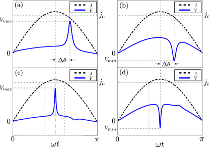
Figure 4: (Color online) Input current $j$ (dashed line) and measured voltage $V$ (solid line) as functions of time $t$. (a) and (b) show the phase delay $\Delta\theta$ between the current maximum and voltage extremum for $C>0$ and $C<0$, respectively. (c) and (d) depict $V(t)$ at $\Delta\theta=0$ for the same $C>0$ and $C<0$, respectively.

Phase shift experiment. Another method to measure the coefficient $C$ is by applying an ac current $j=j_{0}\sin\omega t$ with $j_{0}>j_{c}$, which has only a short time interval where $j>j_{c}$, so that there is only one period of voltage within the period of $j(t)$. One can measure the phase delay, $\Delta\theta$, between the current maximum and voltage extremum (see Fig. 4). Next, one fixes the amplitude $j_{0}$ and tunes the frequency $\omega$ until $\Delta\theta=0$. In this case, for $j_{0}-j_{c}\ll j_{c}$, we can use half of the time interval for which the current pulse is above $j_{c}$ to approximate the period of $\phi$ by dc current $j_{0}$ as

$$\frac{1}{2\omega}\left(\pi-2\arcsin\frac{j_{c}}{j_{0}}\right)\approx\frac{\pi}{|C|\sqrt{j_{0}^{2}-j_{c}^{2}}}.$$ (13)

For $j_{0}-j_{c}\ll j_{c}$, Eq. (13) can be further simplified to give

$$|C|\approx\frac{\pi\omega}{2(j_{0}-j_{c})}.$$ (14)

In other words, when $\omega\approx C(j_{0}-j_{c})$ which corresponds roughly to $\omega\sim 10^{7}$ Hz, the current pulse covers only one period of voltage. Our simulations show that the expression (14) works sufficiently well for $j_{0}\lesssim 1.3j_{c}$. The sign of $C$ is determined by the extremum of the measured voltage: $C>0$ if $V$ has the minimum and $C<0$ if $V$ has the maximum.

Our simulations show (Fig. 4) that in addition to the large peak (dip) of voltage there is a smaller one with the opposite curvature. This is because when $j(t)$ reaches $j_{c}$, the angle $\phi$ has not yet rotated to the angle corresponding to $\sin(2\phi_{0})=1$ due to the cumulative phase delay between current and voltage.

Abrupt current pulse experiment. It is also possible to measure the coefficient $C$ for currents below the critical value $j_{c}$. The constant $|C|j_{c}$ determines the internal time scale of the DW motion. After one switches the subcritical current off at time $t_{i}$, the voltage asymptotically decays as $\exp(-2|C|j_{c}t)$, see Fig. 5. To measure the decay of $V(t)$ with time, one inputs a dc current below $j_{c}$, then measures voltage $V_{i}$ immediately after turning off the current at $t_{i}$, and then later measures voltage $V_{f}$ at time $t_{i}+\Delta_{t}$. We note that right after turning off the current, there is a short time period when the DW dynamics cannot be described by Eqs. (2) and (3). It corresponds to the dynamics of fast degrees of freedom. This process has a characteristic time $\sim 10^{-11}s$ which is typically much smaller than the voltage decay time $\sim 10^{-8}$ s. Thus we can safely assume that the rotation angle $\phi$ does not change much during this time interval, and we find

$$|C|\simeq\frac{1}{2\Delta_{t}j_{c}}\ln\frac{2V_{i}/V_{f}}{1+\sqrt{1-j^{2}/j_{c}^{2}}},$$ (15)

which is valid for $V_{i}/V_{f}\gg 1$. For example, estimating $V_{i}/V_{f}=10$ we find $|C|\approx 1.17/(\Delta_{t}j_{c})$. The sign of $C$ can be easily determined by the form of voltage decay (see Fig. 5).

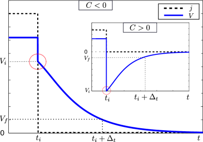
Figure 5: (Color online) Voltage (solid line) evolution after the current (dashed line) is turned off at time $t_{i}$ for $C>0$ given by $\alpha=0.02$ and $\beta=0.01$. Inset: the same dependencies for $C<0$ given by $\alpha=0.01$ and $\beta=0.02$. The measurement of $V_{f}$ is performed at $t_{i}+\Delta_{t}$. The region encircled by the dotted line cannot be described within our approach but it is too small to effect our results.

To summarize, we propose several all-electric measurements of the parameters fully describing domain-wall dynamics in thin ferromagnetic nanowires. These measurements are based on the voltage induced by a moving DW in response to certain current pulses. Our proposal opens doors for experiments which are suitable not only for all-electric DW manipulation but also for the simultaneous measurement of the DW dynamics. These findings give a more reliable and straightforward experimental method to determine the DW dynamics parameters, which can then be compared to microscopic theories. The procedure we described works for a given temperature regime. It may also be used to investigate the temperature dependence of the effective parameters. Future work will include accounting for pinning effects, which brake translational invariance in the wires. future2

We thank I. V. Roshchin, J. Sinova, and E. K. Vehstedt for valuable discussions. This work was supported by the NSF Grant No. 0757992 and Welch Foundation (A-1678).

References

- (1) A. Yamaguchi, T. Ono, S. Nasu, K. Miyake, K. Mibu, and T. Shinjo, Phys. Rev. Lett. 92, 077205 (2004)
- (2) L. Thomas, M. Hayashi, X. Jiang, R. Moriya, C. Rettner, and S. S. P. Parkin, Nature 443, 197 (2006)
- (3) L. Thomas, M. Hayashi, X. Jiang, R. Moriya, C. Rettner, and S. Parkin, Science 315, 1553 (2007)
- (4) G. Meier, M. Bolte, R. Eiselt, B. Krüger, D.-H. Kim, and P. Fischer, Phys. Rev. Lett. 98, 187202 (2007)
- (5) J. Rhensius, L. Heyne, D. Backes, S. Krzyk, L. J. Heyderman, L. Joly, F. Nolting, and M. Kläui, Phys. Rev. Lett. 104, 067201 (2010)
- (6) D. Ilgaz, J. Nievendick, L. Heyne, D. Backes, J. Rhensius, T. A. Moore, M. A. Niño, A. Locatelli, T. O. Menteş, A. v. Schmidsfeld, A. v. Bieren, S. Krzyk, L. J. Heyderman, and M. Kläui, Phys. Rev. Lett. 105, 076601 (2010)
- (7) C. T. Boone, J. A. Katine, M. Carey, J. R. Childress, X. Cheng, and I. N. Krivorotov, Phys. Rev. Lett. 104, 097203 (2010)
- (8) S. A. Yang, G. S. D. Beach, C. Knutson, D. Xiao, Q. Niu, M. Tsoi, and J. L. Erskine, Phys. Rev. Lett. 102, 067201 (2009)
- (9) See, e.g., G.S.D. Beach, M. Tsoi, and J.L. Erskine, J. Magn. Magn. Mater. 320, 1272 (2008) and references therein.
- (10) P. Yan and X. R. Wang, Appl. Phys. Lett. 96, 162506 (2010)
- (11) P. Yan, Z. Z. Sun, J. Schliemann, and X. R. Wang, Europhys. Lett. 92, 27004 (2010)
- (12) S. A. Yang, G. S. D. Beach, C. Knutson, D. Xiao, Z. Zhang, M. Tsoi, Q. Niu, A. H. MacDonald, and J. L. Erskine, Phys. Rev. B 82, 054410 (2010)
- (13) G. S. D. Beach, C. Nistor, C. Knutson, M. Tsoi, and J. L. Erskine, Nature Mat. 4, 741 (2005)
- (14) M. Kläui, P.-O. Jubert, R. Allenspach, A. Bischof, J. A. C. Bland, G. Faini, U. Rüdiger, C. A. F. Vaz, L. Vila, and C. Vouille, Phys. Rev. Lett. 95, 026601 (2005)
- (15) Y. Tserkovnyak and M. Mecklenburg, Phys. Rev. B 77, 134407 (2008)
- (16) R. A. Duine, Phys. Rev. B 79, 014407 (2009)
- (17) A. Singh, S. Mukhopadhyay, and A. Ghosh, Phys. Rev. Lett. 105, 067206 (2010)
- (18) Z. Li and S. Zhang, Phys. Rev. Lett. 92, 207203 (2004)
- (19) A. Thiaville, Y. Nakatani, J. Miltat, and Y. Suzuki, Europhys. Lett. 69, 990 (2005)
- (20) It results in crystalline anisotropy, Dzyaloshinskii-Moriya interaction, etc.
- (21) G. Tatara and H. Kohno, Phys. Rev. Lett. 92, 086601 (2004)
- (22) O. A. Tretiakov and Ar. Abanov, Phys. Rev. Lett. 105, 157201 (2010)
- (23) O. A. Tretiakov, Y. Liu, and Ar. Abanov, Phys. Rev. Lett. 105, 217203 (2010)
- (24) M. Kläui et al., Phys. Rev. Lett. 94, 106601 (2005)
- (25) L. Heyne, J. Rhensius, A. Bisig, S. Krzyk, P. Punke, M. Kläui, L. J. Heyderman, L. L. Guyader, and F. Nolting, Appl. Phys. Lett. 96, 032504 (2010)
- (26) For the Hamiltonian of Ref. \rev@citealpnumTretiakov_DMI this constant is which reduces to for .
- (27) O. A. Tretiakov and Ar. Abanov, (unpublished)
- (28) For the Hamiltonian used in Ref. \rev@citealpnumTretiakov_DMI, , , , and , where and are, respectively, the Dzyaloshinskii-Moriya and exchange interaction constants.
- (29) Since in majority of materials both and , we can be safely neglect compared to 1 in Eq. (8\@@italiccorr).
- (30) O. A. Tretiakov, Y. Liu, and Ar. Abanov, J. Appl. Phys. 109, 07D505 (2011)
- (31) Our simulations show that the initial phase of angle does not affect the phase delay, since the time it takes for the current to increase from to is long enough to adjust the initial angle to the one corresponding to .
- (32) Y. Liu, O. A. Tretiakov, and Ar. Abanov, (unpublished)