Reservoirs of Stability: Flux Tubes in the Dynamics of Cortical Circuits

Abstract

Triggering a single additional spike in a cerebral cortical neuron was recently demonstrated to cause a cascade of extra spikes in the network that is likely to rapidly decorrelate the network’s microstate. The mechanisms involved in this extreme sensitivity of cortical networks are currently not well understood. Here, we show in a minimal model of cortical circuit dynamics that exponential state separation after single spike and even single synapse perturbations coexists with dynamical stability to infinitesimal state perturbations. We propose a unifying picture of exponentially separating flux tubes enclosing unique stable trajectories composing the networks’ state spaces.

Understanding the dynamical characteristics of cerebral cortex networks is fundamental for the understanding of sensory information processing in the brain. Bottom-up investigations of different generic neuronal network models have led to a variety of results ranging from stable key-Zillmer ; key-Jahnke ; key-stable to chaotic dynamics key-VreeswijkSompolinsky ; key-chaos ; key-Latham . In top-down attempts to construct classification and discrimination systems with such networks, the ’edge of chaos’ was proposed to be computationally optimal key-edge . Near this transition between ordered and chaotic dynamics, a network can combine the fading memory and the separation property, both of which are important for the efficacy of computing applications key-reservoir . While fading memory (information about perturbations of the microstate die out over time) is achieved by a stable dynamics, the separation property (distinguishable inputs lead to significantly different macrostates) is best supported by a chaotic dynamics.

Widely used in reservoir computing key-reservoir and one of the most simple models of cortical circuits are networks of randomly coupled inhibitory leaky integrate and fire (LIF) neurons key-Burkitt2006 . These networks exhibit stable chaos, characterized by stable dynamics with respect to infinitesimal perturbations despite an irregular network activity key-Zillmer ; key-Jahnke . They thus exhibit fading memory. Whether and how such networks realize the separation property is however unclear.

Motivated by the recent observation that real cortical networks are highly sensitive to single spike perturbations key-Latham , we examine in this letter how single spike and single synapse perturbations evolve in a formally stable model of generic cortical circuits. We show that random networks of inhibitory LIF neurons exhibit negative definite Lyapunov spectra, confirming the existence of stable chaos. The Lyapunov spectra are invariant to the network size, indicating that stable dynamics is representative for large networks, extensive and preserved in the thermodynamic limit. Remarkably, in the limit of large connectivity, perturbations decay as fast as in uncoupled neurons. Single spike perturbations induce only minute firing rate responses but surprisingly lead to exponential state separation causing complete decoherence of the networks’ microstates within milliseconds. By examining the transition from unstable dynamics to stable dynamics for arbitrary perturbation size, we derive a picture of tangled flux tubes composing the networks’ phase space. These flux tubes form reservoirs of stability enclosing unique stable trajectories, whereas adjacent trajectories separate exponentially fast. In the thermodynamic limit the flux tubes become vanishingly small, implying that even in the limit of infinitesimal weak perturbations the dynamics would be unstable. This contradicts the prediction from the Lyapunov spectrum analysis and reveals that characterizing the dynamics of such networks qualitatively depends on the order in which the weak perturbation limit and the thermodynamic limit are taken.

We studied large sparse networks of $N$ LIF neurons arranged on directed Erdös-Rényi random graphs of mean indegree $K$. The neurons’ membrane potentials $V_{i}\in(-\infty,V_{\textrm{T}})$ with $i=1\dots N$ satisfy

$$\tau_{m}\dot{V}_{i}=-V_{i}+I_{i}(t)$$ (1)

between spike events. When $V_{i}$ reaches the threshold $V_{T}\equiv 1$, neuron $i$ emits a spike and $V_{i}$ is reset to $V_{R}\equiv 0$. The membrane time constant is denoted $\tau_{m}$. The synaptic input currents are

$$I_{i}(t)=\sqrt{K}I_{0}-\frac{J_{0}}{\sqrt{K}}\tau_{m}\sum_{j\in\textrm{pre}(i)}\sum_{s}\delta(t-t_{j}^{(s)}),$$ (2)

composed of constant excitatory external currents $\sqrt{K}I_{0}$ and inhibitory nondelayed $\delta$ pulses of strength $-J_{0}/\sqrt{K}$, received at the spike times $t_{j}^{(s)}$ of the presynaptic neurons $j\in\textrm{pre}(i)$. The external currents $I_{0}$ were chosen to obtain a target network-averaged firing rate $\bar{\nu}$.

Equivalent to the voltage representation, Eq. (1), is a phase representation in which each neuron is described by a phase $\phi_{i}\in[-\infty,1]$, obtained through $\phi_{i}=-\ln\bm{(}(V_{i}-\sqrt{K}I_{0})/(V_{R}-\sqrt{K}I_{0})\bm{)}/T_{i}^{\textrm{free}}$ (where $T_{i}^{\textrm{free}}=-\ln\bm{(}(V_{T}-\sqrt{K}I_{0})/(V_{R}-\sqrt{K}I_{0})\bm{)}$ is the interspike interval of an isolated neuron), with a constant phase velocity and the phase transition curve $U(\phi_{i})=-\ln\bm{(}\exp(-\phi_{i}T_{i}^{\textrm{free}})+J_{0}/(KI_{0})\bm{)}/T_{i}^{\textrm{free}}$ describing the phase updates at spike reception. The neurons’ phases thus evolve, from time $t_{s-1}$ after the last spike in the network through the next spike time $t_{s}$, at which neuron $j^{*}$ fires, according to the map

$$\phi_{i}(t_{s})=\begin{cases}\phi_{i}(t_{s-1})+(t_{s}-t_{s-1})/T_{i}^{\textrm{free}}&\mathrm{for}\,i\neq i^{*}\\ U\bm{(}\phi_{i}(t_{s-1})+(t_{s}-t_{s-1})/T_{i}^{\textrm{free}}\bm{)}&\mathrm{for}\,i=i^{*}.\end{cases}$$ (3)

The neurons postsynaptic to the spiking neuron $j^{*}$ are $i^{*}\in\mathrm{post}\,(j^{*})$. We used the exact phase map (3) for numerically exact event-based simulations and to analytically calculate the single spike Jacobian $\mathbf{D}(t_{s})=\frac{\partial\vec{\phi}(t_{s})}{\partial\vec{\phi}(t_{s-1})}$:

$$D_{ij}(t_{s})=\begin{cases}d_{i^{*}}(t_{s})&\mathrm{for}\,i=j=i^{*}\\ 1-d_{i^{*}}(t_{s})&\mathrm{for}\,i=i^{*},\,j=j^{*}\\ \delta_{ij}&\mathrm{otherwise}.\end{cases}$$ (4)

This matrix depends on the spiking neuron $j^{*}$ and on the phases of the spike receiving neurons $i^{*}$ through the derivative of the phase transition curve $d_{i^{*}}(t_{s})=\partial_{\phi}U\bm{(}\phi_{i^{*}}(t_{s}^{-})\bm{)}$ evaluated at time $t_{s}^{-}$ just before spike reception key-supplement . Describing the evolution of infinitesimal phase perturbations, the single spike Jacobians (4) were used for numerically exact calculations of all Lyapunov exponents $\lambda_{1}\geq\dots\geq\lambda_{N}$ in a standard reorthogonalization procedure key-Benettin1980 .

Figure 1: The balanced state in inhibitory LIF networks: (a) Asynchronous irregular spike pattern of 30 randomly chosen neurons, (b) fluctuating voltage trace of one neuron (voltage increased to $V=2$ at spikes), (c),(d) broad distributions of individual neurons’ firing rates $\nu$ and coefficients of variation $\mathrm{cv}$, (e) network-averaged firing rate $\bar{\nu}$ and synchrony measure $\chi$ versus predicted rate $\bar{\nu}_{\textrm{bal}}=I_{0}/(J_{0}\tau_{m})$ (dotted line: guide to the eye for $\bar{\nu}=\bar{\nu}_{\textrm{bal}}$, $\chi=\frac{\mathrm{STD}([\phi_{i}])}{[\mathrm{STD}(\phi_{i})]}$ where $[\cdot]$ denotes population average), (parameters: $N=10\,000$, $K=1000$, $\bar{\nu}=10\,\textrm{Hz}$, $J_{0}=1$, $\tau_{\textrm{m}}=10\,\textrm{ms}$).

As expected from the construction of the LIF networks, the dynamics converged to a balanced state. Figure 1 shows a representative spike pattern and voltage trace illustrating the irregular and asynchronous firing and strong membrane potential fluctuations. A second characteristic feature of balanced networks is a substantial heterogeneity in the spike statistics across neurons, indicated by broad distributions of coefficients of variation (cv) and firing rates ($\nu$). Independent of model details, the network-averaged firing rate $\bar{\nu}$ in the balanced state can be predicted as $\bar{\nu}_{\textrm{bal}}\approx I_{0}/(J_{0}\tau_{\textrm{m}})$ key-supplement . The good agreement of this prediction with the numerically obtained firing rate confirms the dynamical balance of excitation and inhibition in the studied networks.

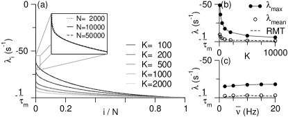
Figure 2: Stable dynamics with respect to infinitesimal perturbations: (a) Spectrum of Lyapunov exponents $\{\lambda_{i}\}$ of networks of $N=10\,000$ LIF neurons for different connectivities $K$, inset: close-up of spectra for $K=100$ and different network sizes $N$, (b),(c) largest Lyapunov exponent $\lambda_{2}=\lambda_{\textrm{max}}$ and mean Lyapunov exponent $\lambda_{\textrm{mean}}=\frac{1}{N}\sum_{i=1}^{N}\lambda_{i}$ versus connectivity $K$ and average firing rate $\bar{\nu}$ (dashed lines: random matrix theory for $\lambda_{\textrm{mean}}$ key-supplement ), (parameters: $N=100\,000$, $K=1000$, $\bar{\nu}=10\,\textrm{Hz}$, $J_{0}=1$, $\tau_{\textrm{m}}=10\,\textrm{ms}$; averages of $10$ initial conditions).

Although the voltage trajectory of each neuron and the network state were very irregular, the collective dynamics of the networks was apparently completely stable (Fig. 2). For all firing rates, coupling strengths and connection probabilities, the whole spectrum of Lyapunov exponents (disregarding the zero exponent for perturbations tangential to the trajectory) was negative, confirming the occurrence of so-called stable chaos in LIF networks key-Zillmer ; key-Jahnke . The invariance of the Lyapunov spectra to the network size $N$, to our knowledge, for the first time demonstrates that this type of dynamics is extensive. With increasing connectivity $K$ all Lyapunov exponents approached a constant $\lambda_{i}\approx-1/\tau_{m}$. This is deduced from the mean Lyapunov exponent given by $\lambda_{\textrm{mean}}\approx-1/\tau_{m}+(V_{T}-\langle V\rangle)/(\sqrt{K}I_{0})+\mathcal{O}(1/K)$ in random matrix approximation and the numerical observation that the largest exponent approached $\lambda_{\mathrm{mean}}$ in the large $K$-limit (key-supplement and Fig.  2(b)). These results suggest that in the thermodynamic limit arbitrary weak perturbations decay exponentially on the single neuron membrane time constant. As will become clear in the following, however, this issue is quite delicate.

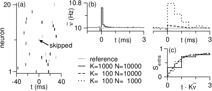
Figure 3: Weak firing rate response after single spike failure: (a) Sample spike pattern of 20 randomly chosen neurons (gray: reference trajectory, black: single spike skipped at $t=0$), (b) network-averaged firing rate of reference trajectory $\bar{\nu}$ and in response to skipped spike $\tilde{\nu}$ versus time for different connectivities $K$ and network sizes $N$, (c) number of extra spikes $S_{\textrm{extra}}=N\int(\tilde{\nu}-\bar{\nu})\textrm{d}t$ in the entire network versus time (rescaled with average input rate $K\bar{\nu}$), (parameters: $\bar{\nu}=10\,\textrm{Hz}$, $J_{0}=1$, $\tau_{\textrm{m}}=10\,\textrm{ms}$; averages of $100$ initial conditions with $10\,000$ calculations each).

Experimentally realizable and well-controlled state perturbations to the dynamics of cortical networks are the addition or suppression of individual spikes key-Latham ; key-Brecht . Such minimalistic neurostimulation can elicit complex behavioral responses key-Brecht and can trigger a measurable rate response in intact cortical networks key-Latham . We therefore examined how such single spike perturbations affected the collective dynamics of our networks. Here, the simplest single spike perturbation is the suppression of a single spike. Figure 3 illustrates the firing rate response if one spike is skipped at $t=0$. The missing inhibition immediately triggered additional spikes in the $K$ postsynaptic neurons such that the network-averaged firing rate increased abruptly by $\delta\bar{\nu}\sim K\bar{\nu}/N$. Since the induced extra spikes inhibited further neurons in the network, the overshoot in the firing rate quickly settled back to the stationary state within a time of order $\delta t\sim 1/(K\bar{\nu})$. The overall number of additional spikes in the networks therefore was $N\delta\bar{\nu}\delta t\approx 1$ and the one skipped spike was immediately compensated by a single extra spike key-supplement .

Figure 4: Sensitivity to single spike failures: (a) Distance $D$ between trajectory after spike failure and reference trajectory versus time in log-lin plots for different connectivities $K$ and average firing rates $\bar{\nu}$, (b) pseudo Lyapunov exponent $\lambda_{p}$ from exponential fits $D\sim\exp(\lambda_{p}t)$ before reaching saturation versus connectivity $K$ and average firing rate $\bar{\nu}$, (c) distance-evolution of all parameter sets (rescaled with approximate perturbation strength $KJ_{0}/\sqrt{K}$) versus time (rescaled with average input rate $K\bar{\nu}$) collapse to characteristic exponential state separation with rate $\lambda_{p}\sim 0.9K\bar{\nu}$ (inset: different network sizes $N$ for $K=100$), (parameters: $N=100\,000$, $K=1000$, $\bar{\nu}=10\,\textrm{Hz}$, $J_{0}=1$, $\tau_{\textrm{m}}=10\,\textrm{ms}$; averages of $10$ initial conditions with $100$ calculations each).

Even though the failure of one individual spike resulted in very weak and brief firing rate responses, it nevertheless induced rapid state decoherence. Figure 4 displays the distance $D(t)=\frac{1}{N}\sum_{i}|\tilde{\phi}_{i}(t)-\phi_{i}(t)|$ between the perturbed trajectory (spike failure at $t=0$) and the reference trajectory. After the spike failure, all trajectories separated exponentially fast at a surprisingly high rate. Because this exponential separation of nearby trajectories is reminiscent of deterministic chaos, we call its separation rate the pseudo Lyapunov exponent $\lambda_{p}$. The pseudo Lyapunov exponent was network size invariant, but showed a completely different behavior compared to the classical Lyapunov exponents. With increasing connectivity, it appears to diverge linearly $\lambda_{p}\sim K\bar{\nu}$. It is thus expected to grow to infinity in the high connectivity limit, reminiscent of binary neuron networks exhibiting an infinite Lyapunov exponent in the thermodynamic limit key-VreeswijkSompolinsky .

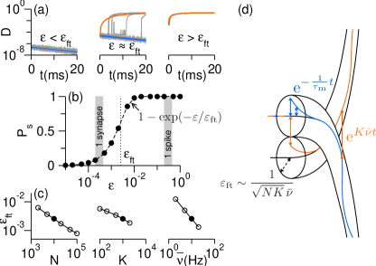
Figure 5: (Color online) Sensitivity to finite-size perturbations: (a) Distance $D$ between perturbed and reference trajectory measured at spike times of reference trajectory (projecting out possible time-shifts) for perturbations of strengths $\varepsilon=0.00002,\,0.002,\,0.2$ in log-lin plots (gray lines: 20 examples for initial perturbations of same size pointing in different random directions perpendicular to trajectory, color lines: averages of exponentially separating/converging cases), (b) probability $P_{s}$ of exponential state separation versus perturbation strength $\varepsilon$ in lin-log plot (dashed line: fit to $P_{s}(\varepsilon)=1-\exp(-\varepsilon/\varepsilon_{\textrm{ft}})$, dotted line: characteristic perturbation size $\varepsilon_{\textrm{ft}}$ separating stable from unstable dynamics, shaded areas: strengths corresponding to single synapse and single spike failures), (c) characteristic perturbation size $\varepsilon_{\textrm{ft}}$ versus network size $N,$ connectivity $K$ and average firing rate $\bar{\nu}$ in log-log plots, (d) symbolic picture of stable flux tubes with radius $\varepsilon_{\textrm{ft}}$ (stable dynamics inside flux tube but exponential separation of adjacent flux tubes), (parameters: $N=10\,000$, $K=1\,000$, $\bar{\nu}=10\,\textrm{Hz}$, $J_{0}=1$, $\tau_{\textrm{m}}=10\,\textrm{ms}$; averages of 10 initial conditions with $100$ calculations and $100$ random directions each).

In the same balanced LIF networks, we thus find stable dynamics in response to infinitesimal perturbations and unstable dynamics in response to single spike failures. To further analyze the transition between these completely opposite behaviors, we applied finite perturbations of variable size perpendicular to the state trajectory (Fig. 5). Depending on the perturbation strength $\varepsilon$ and direction $\overrightarrow{\delta\phi}$ (with $\sum_{i}\delta\phi_{i}^{2}=1$), the perturbed trajectory either converged back to the reference trajectory or diverged exponentially fast. The probability $P_{s}(\varepsilon)$ that a perturbation of strength $\varepsilon$ induced exponential state separation was very well-fitted by $P_{s}(\varepsilon)=1-\exp(-\varepsilon/\varepsilon_{\textrm{ft}})$. Hence, $\varepsilon_{\textrm{ft}}$ is a characteristic phase space distance separating stable from unstable dynamics. Intriguingly, this distance decreased as $\varepsilon_{\textrm{ft}}\sim 1/(\sqrt{KN}\bar{\nu})$. For large $K$ and $N$ the dynamics in the thermodynamic limit ($N\to\infty$) would be unstable even to infinitesimal perturbations ($\varepsilon\to 0$). Contrary, the analysis of the Lyapunov spectra has shown that taking the limit $\varepsilon\to 0$ first and then $N\to\infty$ yields stable dynamics. Thus, the order of the limits appears crucial in defining the dynamical nature of balanced LIF networks.

The evolution of finite perturbations suggests a picture of stable flux tubes around unique trajectories (Fig. 5(d)). Perturbations within these flux tubes decayed exponentially, whereas perturbations greater than the typical flux tube radius $\varepsilon_{\textrm{ft}}\sim 1/(\sqrt{KN}\bar{\nu})$ induced exponential state separation. Single synaptic failures correspond to small perturbations of size $\varepsilon_{\textrm{syn}}\approx J_{0}/\sqrt{KN}$ and therefore had a $N$ and $K$ independent probability of inducing exponential state separation. This probability increased linearly with the average firing rate $\bar{\nu}$ key-supplement .

Summarizing, our analysis revealed the co-occurence of dynamical stability to infinitesimal state perturbations and sensitive dependence on single spike and even single synapse perturbations in the dynamics of networks of inhibitory LIF neurons in the balanced state. They exhibit a negative definite extensive Lyapunov spectrum that at first sight suggests a well-defined thermodynamic limit of the network dynamics characterized by stable chaos as previously proposed key-Zillmer ; key-Jahnke . In this dynamics, single spike failures induce extremely weak firing rate responses that become basically negligible for large networks. Nevertheless, such single spike perturbations typically put the network state on a very different dynamical path that diverges exponentially from the original one. The rate of exponential state separation was quantified with the so called pseudo Lyapunov exponent $\lambda_{p}$. The scaling of $\lambda_{p}\sim K\bar{\nu}$ implies extremely rapid, practically instantaneous, decorrelation of network microstates. Our results suggest that the seemingly paradoxical coexistence of local stability and exponential state separation reflects the partitioning of the networks’ phase space into a tangle of flux tubes. States within a flux tube are attracted to a unique, dynamically stable trajectory. Different flux tubes, however, separate exponentially fast. The decreasing flux tube radius in the large system limit suggests that an unstable dynamics dominates the thermodynamic limit. The resulting sensitivity to initial conditions is described by the rate of flux tube separation, the pseudo Lyapunov exponent, that showed no sign of saturation. These findings suggest that the previously reported infinite Lyapunov exponent on the one hand key-VreeswijkSompolinsky and local stability on the other hand key-Zillmer ; key-Jahnke resulted from the order in which the weak perturbation limit and the thermodynamic limit were taken.

For finite networks, the phase space structure revealed here may provide a basis for insensitivity to small perturbations (e.g. noise or variations in external inputs) and strong sensitivity to larger perturbations. In the context of reservoir computing, the flux tube radius defines a border between the fading property (variations of initial conditions smaller $\varepsilon_{\mathrm{ft}}$ die out exponentially) and the separation property (input variations larger $\varepsilon_{\mathrm{ft}}$ cause exponentially separating trajectories). Applications of LIF neuron networks in reservoir computing may thus strongly benefit if the flux tube structure of the network phase space is taken into account. Our results of a very high pseudo Lyapunov exponent also reveal that the notion of an ’edge of chaos’ is not applicable in these networks.

We thank E. Bodenschatz, T. Geisel, S. Jahnke, J. Jost, P. E. Latham, R. M. Memmesheimer, H. Sompolinsky, M. Timme and C. van Vreeswijk for fruitful discussions. This work was supported by BMBF (01GQ07113, 01GQ0811), GIF (906-17.1/2006), DFG (SFB 889) and the Max Planck Society.

References

- (1) R. Zillmer et al. Phys. Rev. E 74, 036203 (2006); R. Zillmer, N. Brunel and D. Hansel, ibid. 79, 031909 (2009).
- (2) S. Jahnke, R. M. Memmesheimer and M. Timme, Phys. Rev. Lett. 100, 048102 (2008); Front. Comput. Neurosci. 3, 13 (2009).
- (3) D. Z. Jin, Phys. Rev. Lett. 89, 208102 (2002).
- (4) C. van Vreeswijk and H. Sompolinsky, Science 274, 1724 (1996); Neural Comput. 10, 1321 (1998).
- (5) H. Sompolinsky, A. Crisanti, and H. J. Sommers, Phys. Rev. Lett. 61, 259 (1988); D. Hansel and H. Sompolinsky, J. Comput. Neurosci. 3, 7 (1996); A. Zumdieck et al., Phys. Rev. Lett. 93, 244103 (2004); A. Banerjee, P. Seriés, and A. Pouget, Neural Comput. 20, 974 (2008); D. Zhou et al., Phys. Rev. E 80, 031918 (2009); S. El Boustani and A. Destexhe, Int. J. Bifurcat. Chaos 20, 1687 (2010); M. Monteforte and F. Wolf, Phys. Rev. Lett. 105, 268104 (2010).
- (6) M. London et al., Nature 466, 123 (2010).
- (7) N. Bertschinger and T. Natschlaeger, Neural Comput. 16, 1413 (2004).
- (8) W. Maass, T. Natschlaeger and H. Markram, Neural Comput. 14, 2531 (2002); H. Jaeger, GMD Report 148 (2001); D. Sussillo and L. F. Abbott, Neuron 63, 544 (2009).
- (9) A. N. Burkitt, Biol. Cybern. 95, 1 (2006); 95, 97 (2006).
- (10) See EPAPS Document No. xxx.yyy for more details.
- (11) G. Benettin et al., Meccanica 15, 21 (1980).
- (12) M. Brecht et al., Nature 427, 704 (2004); D. Huber et al., Nature 451, 61 (2008); A. R. Houweling and M. Brecht, Nature 451, 65 (2008).