Natural PQ symmetry in the 3-3-1 model with a minimal scalar sector

Abstract

In the framework of a 3-3-1 model with a minimal scalar sector we make a detailed study concerning the implementation of the PQ symmetry in order to solve the strong CP problem. For the original version of the model, with only two scalar triplets, we show that the entire Lagrangian is invariant under a PQ-like symmetry but no axion is produced since an $U(1)$ subgroup remains unbroken. Although in this case the strong CP problem can still be solved, the solution is largely disfavored since three quark states are left massless to all orders in perturbation theory. The addition of a third scalar triplet removes the massless quark states but the resulting axion is visible. In order to become realistic the model must be extended to account for massive quarks and invisible axion. We show that the addition of a scalar singlet together with a $Z_{N}$ discrete gauge symmetry can successfully accomplish these tasks and protect the axion field against quantum gravitational effects. To make sure that the protecting discrete gauge symmetry is anomaly free we use a discrete version of the Green–Schwarz mechanism.

I Introduction

The standard model (SM) of the elementary particles physics successfully describes almost all of the phenomenology of the strong, electromagnetic, and weak interactions. However, from the experimental point of view, the need to go to physics beyond the standard model comes from the neutrino masses and mixing, which are required to explain the solar and atmospheric neutrino data. On the other hand, from the theoretical point of view, the SM can not be taken as the fundamental theory since some important contemporary questions, like the number of generations of quarks and leptons, do not have an answer in its context. Unfortunately we do not know what the physics beyond the SM should be. A likely scenario is that at the TeV scale physics will be described by models which, at least, give some insight into the unanswered questions of the SM.

A way of introducing new physics is to enlarge the symmetry gauge group. For example, the gauge symmetry may be $SU(3)_{C}\otimes SU(3)_{L}\otimes U(1)_{X}$, instead of that of the SM. Models based on this gauge group have become known as 3-3-1 models pisano1992 ; frampton1992 ; foot1994 . Although the 3-3-1 models coincide with the SM at low energies, they explain some fundamental questions. This is the case of the number of generations cited above. In the 3-3-1 model framework, the number of generations must be three, or multiple of three, in order to cancel anomalies. This is because the model is anomaly-free only if there is an equal number of triplets and antitriplets, including the color degrees of freedom. In this case, each generation is anomalous. The anomaly cancelation only occurs for the three, or multiply of three, generations together, and not generation by generation like in the SM. This provides, at least, a first step towards the understanding of the flavor question. Other interesting features of the 3-3-1 models concern the electric charge quantization and the vectorial character of the electromagnetic interaction. These questions can be accommodated in the SM. However, in the 3-3-1 models these questions are related one to another and are independent of the nature of the neutrinos.

In recent literature we find studies about the most different aspects of the 3-3-1 model phenomenology. Among others, a fundamental puzzling aspect is: Why is the CP nonconservation in the strong interactions so small Pal1995 ; alex2004 ? The last question, quantified by the $\overline{\theta}$ parameter of the effective QCD Lagrangian, is known as the strong CP problem. Several solutions based on different ideas have been proposed. According to the framework, they are based on: unconventional dynamics shaposhnikov1988 , spontaneously broken CP barr1984 ; barr1986 ; nelson1984 , and an additional chiral symmetry. In the framework of introducing an additional chiral symmetry, two suggestions have been made. If this symmetry is not broken, the symmetry is realized in the Wigner-Weyl manner and the only possible way of relating this unbroken chiral symmetry with flavor conserving gluons is to have at least one massless quark kaplan1986 . This suggestion is disfavored by standard current algebra analysis gasser1982 ; Nelson . The second possibility is that the global $U\left(1\right)$ chiral symmetry, known as $U\left(1\right)_{\text{PQ}}$ peccei1997 ; peccei1977 , is spontaneously broken down which implies a Nambu-Goldstone boson (NG boson), currently known as the axion kim1979 ; dine1981 ; zhitnitsky1980 .

In this paper we consider the strong CP problem in the framework of a version of the 3-3-1 model in which the scalar sector is minimal Long . This model has become known as the “economical 3-3-1 model”. The appealing feature of this 3-3-1 model is the natural existence of a PQ-like $U\left(1\right)$ symmetry. To study the consequences of this symmetry into this model, we organize this paper as follows: in Sec. II we briefly describe the model, in Sec. III we analyze the consequences of the natural PQ-like symmetry into the model and find that the symmetry is realized in the Wigner-Weyl manner implying three massless quarks, what is in disagree with the standard current algebra analysis. Thus, we propose the introduction of two new scalar fields, $\eta$ and $\phi$, in order to both give a solution to the massless quarks and implement the PQ mechanism. Since this mechanism need that the $U(1)_{\text{ PQ}}$ be anomalous in order to solve the strong CP problem, it seems not natural to impose this symmetry to the Lagrangian. However, it could be understood as being natural if it is a residual symmetry of a larger one which is not anomalous and spontaneously broken. Then, we consider a $Z_{N}$ discrete gauge symmetry to be a symmetry of the Lagrangian. The discrete gauge anomalies are canceled by a discrete version of the Green-Schwarz mechanism. After, two $Z_{N}$ symmetries, $Z_{10}$ and $Z_{11}$, which protect the axion against quantum gravity effects, are explicitly shown. Finally, our conclusions are given in Sec. IV.

II A brief review of the economical 3-3-1 model

The different models based on a 3-3-1 gauge symmetry can be classified according to the electric charge operator

$$Q=T^{3}-bT^{8}+X\text{,}$$ (1)

where $T^{3}$ and $T^{8}$ are the diagonal Gell-Mann matrices, $X$ refers to the quantum number of the $U\left(1\right)_{X}$ group, and $b=1/\sqrt{3}$, $\sqrt{3}$. The embedding $b$ parameter defines the model. Here, we will consider the model with both $b=1/\sqrt{3}$ and the simplest scalar sector, which was proposed for the first time in Ref. ponce . It has become known in the literature as “economical 3-3-1 model”. This model had origin in a systematic study of all possible 3-3-1 models without exotic electric charges ponce2002 .

To give a brief review of the main features of this model, let us say that it has a fermionic matter content given by

$$\Psi_{aL} =\left(\nu_{a},e_{a},\left(\nu_{aR}\right)^{C}\right)_{L}^{T}\sim\left(\mathbf{1},\mathbf{3},-1/3\right)\text{,}\quad e_{aR}\sim\left(\mathbf{1},\mathbf{1},-1\right)\text{,}$$

$$Q_{\alpha L} =\left(d_{\alpha},u_{\alpha},d_{\alpha}^{\prime}\right)_{L}^{T}\sim\left(\mathbf{3},\mathbf{3}^{\ast},0\right)\text{,}\quad Q_{3L}=\left(u_{3},d_{3},u_{3}^{\prime}\right)_{L}^{T}\sim\left(\mathbf{\ \ 3},\mathbf{3},1/3\right)\text{,}$$

$$u_{aR} \sim\left(\mathbf{3},\mathbf{1},2/3\right)\text{,}\quad u_{3R}^{\prime}\sim\left(\mathbf{3},\mathbf{1},2/3\right)\text{, }$$

$$d_{aR} \sim(\mathbf{3},\mathbf{1},-1/3)\text{,}\quad d_{\alpha R}^{\prime}\sim\left(\mathbf{3},\mathbf{1},-1/3\right)\text{,}$$ (2)

where $a=1$, $2$, $3$, $\alpha=1$, $2$ (from now on Latin and Greek letters always take the values $1$, $2$, $3$ and $1$, $2$, respectively) and the values in the parentheses denote quantum numbers based on the $\left(SU\left(3\right)_{C},SU\left(3\right)_{L},U\left(1\right)_{X}\right)$ factor, respectively. In this model the electric charges of the exotic quarks are the same as the usual ones, i.e. $Q\left(d_{\alpha}^{\prime}\right)=-1/3$ and $Q\left(u_{3}^{\prime}\right)=2/3$.

In the bosonic matter content there are only two scalar triplets, $\chi$ and $\rho$

$$\chi=\left(\chi^{0},\chi^{-},\chi_{1}^{0}\right)^{T}\sim\left(\mathbf{1},\mathbf{3},-1/3\right)\text{,}\quad\rho=\left(\rho^{+},\text{ }\rho^{0},\text{ }\rho_{1}^{+}\right)\sim\left(\mathbf{1},\mathbf{3},2/3\right)\text{.}$$ (3)

These two scalar broken down spontaneously the $SU\left(3\right)_{L}\otimes U\left(1\right)_{X}$ gauge group. The vacuum expection values, vevs, in this model satisfy the constraint

$$V_{\rho^{0}}\equiv\left\langle\text{Re\thinspace}\rho^{0}\right\rangle\text{, }V_{\chi^{0}}\equiv\left\langle\text{Re\thinspace}\chi^{0}\right\rangle\ll V_{\chi_{1}^{0}}\equiv\left\langle\text{ Re\thinspace}\chi_{1}^{0}\right\rangle\text{.}$$

With the quark, lepton and scalar multiplets above we have the Yukawa interactions

$$\mathcal{L}_{\text{Y}}^{l} =Y_{ab}\overline{\Psi_{aL}}e_{bR}\rho+Y_{ab}^{\prime}\epsilon^{ijk}\left(\overline{\Psi_{aL}}\right)_{i}\left(\Psi_{bL}\right)_{j}^{C}\left(\rho^{\ast}\right)_{k}+\text{ H.c.,}$$ (4)

$$\mathcal{L}_{\text{Y}}^{q} =G^{1}\overline{Q_{3L}}u_{3R}^{\prime}\chi+G_{\alpha\beta}^{2}\overline{Q_{\alpha L}}d_{\beta R}^{\prime}\chi^{\ast}+G_{a}^{3}\overline{Q_{3L}}d_{aR}\rho$$

$$+G_{\alpha a}^{4}\overline{Q_{\alpha L}}u_{aR}\rho^{\ast}+G_{a}^{5}\overline{Q_{3L}}u_{aR}\chi+G_{\alpha a}^{6}\overline{Q_{\alpha L}}d_{aR}\chi^{\ast}$$

$$+G_{\alpha}^{7}\overline{Q_{3L}}d_{\alpha R}^{\prime}\rho+G_{\alpha}^{8}\overline{Q_{\alpha L}}u_{3R}^{\prime}\rho^{\ast}+\text{H.c.,}$$ (5)

for leptons and quarks respectively. $Y_{ab}$ and $G^{i}$ are arbitrary complex matrices and $Y_{ab}^{\prime}$ is an antisymmetric matrix. We use the convention that an addition over repeated indices is implied. Notice that the Yukawa interactions given in Eqs. (4) and (5) are the most general allowed by the gauge symmetries. Here, we follow exactly the Refs. Long and long2006 , i.e. none additional symmetries are imposed, contrarily to what is done in the Ref. ponce2006 where a $Z_{2}$ symmetry is imposed.

The most general scalar potential invariant under the gauge symmetry is

$$V_{\text{H}} =\mu_{\chi}^{2}\chi^{\dagger}\chi+\mu_{\rho}^{2}\rho^{\dagger}\rho+\lambda_{1}\left(\chi^{\dagger}\chi\right)^{2}+\lambda_{2}\left(\rho^{\dagger}\rho\right)^{2}$$

$$+\lambda_{3}\left(\chi^{\dagger}\chi\right)\left(\rho^{\dagger}\rho\right)+\lambda_{4}\left(\chi^{\dagger}\rho\right)\left(\rho^{\dagger}\chi\right)\text{.}$$ (6)

One of the main features of this model is that its scalar sector is the simplest possible. In principle, this should make the scalar potential analysis easier. A study of the stability of this scalar potential is presented in Ref. ponce2009 .

III $U(1)_{\text{PQ}}$ symmetry in the economical 3-3-1 model

An $U\left(1\right)_{\text{PQ}}$ symmetry is global and chiral peccei1997 ; peccei1977 , i.e. it treats the left- and right-handed parts of a Dirac field differently. Moreover, it must be both a symmetry of the entire Lagrangian and valid only at the classical level. In renormalizable theories, the key ingredient of the $U(1)_{\text{PQ}}$ is that it must be afflicted by a color anomaly, i.e. its associated current, $j_{\mu}^{\text{ PQ}}$, must obey

$$\partial^{\mu}j_{\mu}^{\text{PQ}}\supset\frac{Ng^{2}}{16\pi^{2}}G\widetilde{G}\text{,}$$ (7)

being $G\widetilde{G}=\frac{1}{2}\epsilon^{\mu\nu\sigma\tau}G_{\mu\nu}^{b}G_{\sigma\tau}^{b}$, and $G_{\mu\nu}^{b}$ is the color field strength tensor $\left(b=1\text{,}...\right.$ $\left.\text{, }8\right)$. $N$ must not be zero.

Now, we are going to prove that the economical 3-3-1 model entire Lagrangian is naturally invariant under an $U(1)_{\text{PQ}}$ symmetry transformation. To do so, we search for how many $U\left(1\right)$ symmetries the model has. First of all, we write the relations that these symmetries must obey in order to keep the entire Lagrangian invariant. From Eqs. (4-6) we obtain the following relations

$$-X_{Q_{3}}+X_{u_{3R}^{\prime}}+X_{\chi} =0\text{,}\qquad-X_{Q}+X_{d_{R}^{\prime}}-X_{\chi}=0\text{,}$$ (8)

$$-X_{Q_{3}}+X_{u_{R}}+X_{\chi} =0\text{,}\qquad-X_{Q}+X_{d_{R}}-X_{\chi}=0\text{,}$$ (9)

$$-X_{Q_{3}}+X_{d_{R}}+X_{\rho} =0\text{,}\qquad-X_{Q}+X_{u_{R}}-X_{\rho}=0\text{,}$$ (10)

$$-X_{Q_{3}}+X_{d_{R}^{\prime}}+X_{\rho} =0\text{,}\qquad-X_{Q}+X_{u_{3R}^{\prime}}-X_{\rho}=0\text{,}$$ (11)

$$-X_{\Psi}+X_{e_{R}}+X_{\rho} =0\text{,}\qquad-2X_{\Psi}-X_{\rho}=0\text{,}$$ (12)

where the notation $X_{\psi}$ above is to be understood as the $U\left(1\right)$ charge of the $\psi$ field. Solving the equations above, we find three independent $U\left(1\right)$ symmetries. One of these is the $U\left(1\right)_{X}$ gauge symmetry. The other two are the usual baryon number symmetry, $U\left(1\right)_{B}$, and a chiral symmetry acting on the quarks, $U\left(1\right)_{\text{PQ}}$. Thus, the model actually has a larger symmetry: $SU\left(3\right)_{C}\otimes SU\left(3\right)_{L}\otimes U\left(1\right)_{X}\otimes U\left(1\right)_{B}\otimes U\left(1\right)_{\text{PQ}}$. The two last symmetries are global. This is summarized in the Table 1.

Table 1: Assignment of quantum charges in the economical 3-3-1 model.

	$Q_{\alpha L}$	$Q_{3L}$	($u_{aR}$, $u_{3R}^{\prime}$)	($d_{aR}$, $d_{\alpha R}^{\prime}$)	$\Psi_{aL}$	$e_{aR}$	$\rho$	$\chi$
$U\left(1\right)_{X}$	$0$	$1/3$	$2/3$	$-1/3$	$-1/3$	$-1$	$2/3$	$-1/3$
$U\left(1\right)_{B}$	$1/3$	$1/3$	$1/3$	$1/3$	$0$	$0$	$0$	$0$
$U\left(1\right)_{\text{PQ}}$	$-1$	$1$	$0$	$0$	$-1/2$	$-3/2$	$1$	$1$

We can see that the $U\left(1\right)_{\text{PQ}}$ chiral symmetry is afflicted by a color anomaly in the following way

$$A_{\text{PQ}}\varpropto-X_{\rho}-2X_{\chi}=-3\text{,}$$ (13)

where $A_{\text{PQ}}$ is the coefficient of the $\left[SU\left(3\right)_{C}\right]^{2}U\left(1\right)_{\text{PQ}}$ anomaly. Therefore, this chiral symmetry is a PQ-like symmetry. Also, notice that in this case the $U\left(1\right)_{\text{PQ}}$ is an accidental symmetry, i.e. it follows from the gauge local symmetry plus renormalizability. In other words, the economical model naturally has a PQ symmetry. The naturalness of the $U\left(1\right)_{\text{PQ}}$ in the economical 3-3-1 model is a key point. In our understanding, since $U\left(1\right)_{\text{PQ}}$ symmetry is anomalous its imposition is not sensible in the sense that in the absence of further constraints on very high energy physics we should expect all relevant and marginally relevant operators that are forbidden only by this symmetry to appear in the effective Lagrangian with coefficient of order one, but if this symmetry follows from some other free anomaly symmetry, in our case from the gauge symmetry, all terms which violate it are then irrelevant in the renormalization group sense.

Unfortunately, when $\chi$ and $\rho$ acquire vacuum expectation values, vevs, different from zero, a subgroup of $U(1)_{X}\otimes U(1)_{\text{PQ}}$ remains unbroken, i.e. the symmetry-breaking pattern is

$$SU\left(3\right)_{L}\otimes U\left(1\right)_{X}\otimes U\left(1\right)_{\text{PQ}}\overset{\langle\chi\rangle}{\longrightarrow}SU\left(2\right)_{L}\otimes U\left(1\right)_{Y}\otimes U\left(1\right)_{\text{PQ}}^{\prime}$$

$$\text{ \ \ \ \ \ \ \ \ \ \ \ \ \ \ \ \ \ \ \ \ \ \ \ \ \ \ \ \ \ \ \ \ \ \ \ \ }\overset{\langle\rho\rangle}{\longrightarrow}U\left(1\right)_{Q}\otimes U\left(1\right)_{\text{PQ}}^{\prime\prime}\text{,}$$ (14)

where $U(1)_{Q}$ is the electromagnetic symmetry. The $SU\left(3\right)_{C}$ and $U(1)_{B}$ groups have been omitted in the expression above because these are both unbroken and irrelevant to the current analysis. An explicit expression of the $U\left(1\right)_{\text{PQ}}^{\prime}$ symmetry can be easily written as

$$U\left(1\right)_{\text{PQ}}^{\prime}\equiv U\left(1\right)_{\text{PQ}}+3U\left(1\right)_{X}\text{.}$$ (15)

Also, note that $U\left(1\right)_{\text{PQ}}^{\prime}$ and $U\left(1\right)_{\text{PQ}}^{\prime\prime}$ are PQ-like symmetries because these are quiral and afflicted by a color anomaly.

As a consequence of the unbroken $U\left(1\right)_{\text{PQ}}^{\prime\prime}$ chiral symmetry (i.e. $U\left(1\right)_{\text{PQ}}^{\prime\prime}$ is realized in the Wigner-Weyl manner), none axion appears in the scalar mass spectrum. Instead of that, some quarks remain massless after the spontaneous symmetry breaking, and these will remain massless to all orders of perturbation theory.

To show the previously said, we explicitly calculate the mass spectra of scalars and quarks. First, we calculate the scalar mass spectrum

$$m_{H_{1},H_{2}}^{2} =\text{$\lambda$}_{1}V_{\rho^{0}}^{2}+\left(V_{\chi^{0}}^{2}+V_{\chi_{1}^{0}}^{2}\right)\text{$\lambda$}_{2}$$

$$\pm\sqrt{\left(V_{\rho^{0}}^{2}\text{$\lambda$}_{1}-\left(V_{\chi^{0}}^{2}+V_{\chi_{1}^{0}}^{2}\right)\text{$\lambda$}_{2}\right)^{2}+\left(V_{\chi^{0}}^{2}+V_{\chi_{1}^{0}}^{2}\right)V_{\rho^{0}}^{2}\text{$\lambda$}_{3}^{2}}\text{,}$$ (16)

$$m_{H_{3}^{\pm}}^{2} =\frac{1}{2}\left(V_{\rho^{0}}^{2}+V_{\chi^{0}}^{2}+V_{\chi_{1}^{0}}^{2}\right)\text{$\lambda$}_{4}\text{,}$$ (17)

where $V_{\rho^{0}}$, $V_{\chi^{0}}$, $V_{\chi_{1}^{0}}$ are the vevs of $\rho^{0}$, $\chi^{0}$, $\chi_{1}^{0}$, respectively. For simplicity, all the vevs have been assumed to be reals. Additionally, there are exactly 8 NG bosons that will become the longitudinal components of the 8 gauge bosons  ponce . The absence of one physical massless state (or axion) in the scalar spectrum shows that the $U\left(1\right)_{\text{PQ}}^{\prime\prime}$ symmetry remaining unbroken after the spontaneous symmetry breaking.

On the other hand, in the quark spectra, there are three massless states, one in the up-quark sector and two in the down-quark sector. First, consider the up quark mass matrix at the tree level which is written as

$$\overline{\mathbf{u}_{L}}M_{u}^{(0)}\mathbf{u}_{R}\equiv\frac{1}{\sqrt{2}}\overline{\mathbf{u}_{L}}\begin{bmatrix}G_{11}^{4}V_{\rho^{0}}&\text{$G_{12}^{4}V_{\rho^{0}}$}&G_{13}^{4}V_{\rho^{0}}&G_{1}^{8}V_{\rho^{0}}\\ G_{21}^{4}V_{\rho^{0}}&G_{22}^{4}V_{\rho^{0}}&G_{23}^{4}V_{\rho^{0}}&G_{2}^{8}V_{\rho^{0}}\\ G_{1}^{5}V_{\chi^{0}}&G_{2}^{5}V_{\chi^{0}}&G_{3}^{5}V_{\chi^{0}}&G^{1}V_{\chi^{0}}\\ G_{1}^{5}V_{\chi_{1}^{0}}&G_{2}^{5}V_{\chi_{1}^{0}}&G_{3}^{5}V_{\chi_{1}^{0}}&G^{1}V_{\chi_{1}^{0}}\end{bmatrix}\mathbf{u}_{R}\text{,}$$ (18)

where $\overline{\mathbf{u}_{L}}\equiv\left(\overline{u_{1L}},\overline{u_{2L}},\overline{u_{3L}},\overline{u_{3L}^{\prime}}\right)$ and $\mathbf{u}_{R}\equiv\left(u_{1R},u_{2R},u_{3R},u_{3R}^{\prime}\right)^{\text{T}}$ . The third and fourth rows of the $M_{u}^{(0)}$ matrix are proportional, thus there is a massless up quark (we call this massless up quark simply as $u$) at the tree level. An analytical expression for this massless state can be given but it is useless for our analysis. Later we give arguments that the $u$ quark remain massless to all orders of perturbation theory banks . Similarly, the down-quark mass matrix at the tree level, $M_{d}^{(0)}$, defined as $\frac{1}{\sqrt{2}}\overline{\mathbf{d}_{L}}M_{d}^{(0)}\mathbf{d}_{R}$, reads

$$\begin{bmatrix}G_{11}^{6}V_{\chi^{0}}\text{ \ }&\text{$G_{12}^{6}V_{\chi^{0}}$ \ }&G_{13}^{6}V_{\chi^{0}}\text{ \ }&G_{11}^{2}V_{\chi^{0}}\text{ \ }&G_{12}^{2}V_{\chi^{0}}\text{ \ }\\ G_{21}^{6}V_{\chi^{0}}\text{ \ }&G_{22}^{6}V_{\chi^{0}}\text{ \ }&G_{23}^{6}V_{\chi^{0}}\text{ \ }&G_{21}^{2}V_{\chi^{0}}\text{ \ }&G_{22}^{2}V_{\chi^{0}}\text{ \ }\\ G_{1}^{3}V_{\rho^{0}}\text{ \ }&G_{2}^{3}V_{\rho^{0}}\text{ \ }&G_{3}^{3}V_{\rho^{0}}\text{ \ }&G_{1}^{7}V_{\rho^{0}}\text{ \ }&G_{2}^{7}V_{\rho^{0}}\text{ \ }\\ G_{11}^{6}V_{\chi_{1}^{0}}\text{ \ }&G_{12}^{6}V_{\chi_{1}^{0}}\text{ \ }&G_{13}^{6}V_{\chi_{1}^{0}}\text{ \ }&G_{11}^{2}V_{\chi_{1}^{0}}\text{ \ }&G_{12}^{2}V_{\chi_{1}^{0}}\text{ \ }\\ G_{21}^{6}V_{\chi_{1}^{0}}\text{ \ }&G_{22}^{6}V_{\chi_{1}^{0}}\text{ \ }&G_{23}^{6}V_{\chi_{1}^{0}}\text{ \ }&G_{21}^{2}V_{\chi_{1}^{0}}\text{ \ }&G_{22}^{2}V_{\chi_{1}^{0}}\text{ \ }\end{bmatrix}\text{,}$$ (19)

where $\overline{\mathbf{d}_{L}}\equiv\left(\overline{d_{1L}},\overline{d_{2L}},\overline{d_{3L}},\overline{d_{1L}^{\prime}},\overline{d_{2L}^{\prime}}\right)$ and $\mathbf{d}_{R}\equiv\left(d_{1R},d_{2R},d_{3R},d_{1R}^{\prime},d_{2R}^{\prime}\right)^{\text{T}}$. Since the first and fourth rows, and the second and fifth rows, are proportional to each other, the $M_{d}^{(0)}$ matrix has two eigenvalues equal to zero (we call these massless down quarks as $d$ and $s$). Thus, the economical model has three massless quark states: one in the up-quark sector and two in the down-quark sector. In other words, the economical 3-3-1 model has a remaining unbroken quiral symmetry, $U\left(1\right)_{\text{PQ}}^{\prime\prime}$ that allows to transform $u_{L}\rightarrow e^{i\alpha}u_{L}$, $d_{L}\rightarrow e^{i\alpha}d_{L}$, $s_{L}\rightarrow e^{i\alpha\gamma}s_{L}$, leaving the Lagrangian invariant. This symmetry will protect these massless quarks to acquire mass at any level of perturbation theory  banks . At this point it is important to say that, since the $U\left(1\right)_{\text{PQ}}^{\prime\prime}$ symmetry is anomalous, these quarks will acquire mass only through QCD non-perturbative effects (for example, by instanton effects Hooft ). Although, the quarks could acquire some mass through these non-perturbative processes, this is in conflict with both chiral QCD and lattice calculation where the ratio $m_{u}/m_{d}$ is $0.410\pm 0.036$ gasser1982 ; Nelson ; kim2009 .

Before considering a possible solution to the problem mentioned above, for the sake of completeness, we find important to say that in the Ref. Long one-loop contributions to the up-quark mass matrix were calculated, even though a subtle flaw makes these contributions no right. To demonstrate that, we exactly follow the same lines of the Ref. Long . There, in the section IV, the authors consider for simplicity, one-loop contributions to the sub-matrix

$$M_{u_{3}u_{3}^{\prime}}^{(0)}\equiv\frac{1}{\sqrt{2}}\begin{bmatrix}G_{3}^{5}V_{\chi^{0}}&\text{ \ \ }G^{1}V_{\chi^{0}}\\ G_{3}^{5}V_{\chi_{1}^{0}}&\text{ \ \ }G^{1}V_{\chi_{1}^{0}}\end{bmatrix}\text{,}$$ (20)

where $M_{u_{3}u_{3}^{\prime}}^{(0)}$ is written in the base $\left(u_{3}\text{, }u_{3}^{\prime}\right)$. The other two massive quark states, $u_{1}$ and $u_{2}$, which acquire mass at tree level ($m_{1}=G_{11}^{4}V_{\rho^{0}}/\sqrt{2}$, $m_{2}=G_{22}^{4}V_{\rho^{0}}/\sqrt{2}$, see Eq.(27) in Ref. Long ) are not important in the analysis. The matrix Eq. (20) mixes together the states $u_{3}$ and $u_{3}^{\prime}$. A combination of them will be a massless quark and the orthogonal combination acquires a mass $\sim V_{\chi_{1}^{0}}$.

Now, the idea is to calculate the one-loop contributions coming from the Feynman diagrams in the Fig. 1 to the up-quark mass sub-matrix defined in Eq. (20).

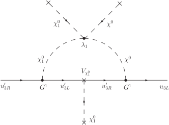
(a) ref1

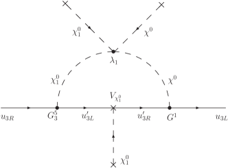
(b) ref2

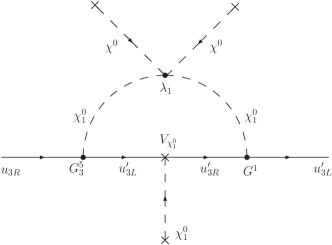
(c) ref3

(d) ref4

Figure 1: One-loop contributions to the up-quark mass matrix.

Following the Ref. Long , we get

$$\Delta_{u_{3L}\text{,}u_{3R}^{\prime}} =-2iV_{\chi^{0}}V_{\chi_{1}^{0}}\lambda_{1}M_{u_{3}^{\prime}}\left(G^{1}\right)^{2}$$

$$\times\int\frac{d^{4}p}{\left(2\pi\right)^{4}}\frac{p^{2}}{\left(p^{2}-M_{u_{3}^{\prime}}^{2}\right)^{2}\left(p^{2}-M_{\chi^{0}}^{2}\right)\left(p^{2}-M_{\chi_{1}^{0}}^{2}\right)}$$

$$\equiv 2V_{\chi^{0}}V_{\chi_{1}^{0}}\lambda_{1}M_{u_{3}^{\prime}}\left(G^{1}\right)^{2}I\left(M_{u_{3}^{\prime}}^{2}\text{, }M_{\chi^{0}}^{2}\text{, }M_{\chi_{1}^{0}}^{2}\right)\text{,}$$ (21)

where $I\left(M_{u_{3}^{\prime}}^{2}\text{, }M_{\chi^{0}}^{2}\text{, }M_{\chi_{1}^{0}}^{2}\right)$ is defined as

$$I\left(M_{u_{3}^{\prime}}^{2}\text{, }M_{\chi^{0}}^{2}\text{, }M_{\chi_{1}^{0}}^{2}\right)\equiv-i\int\frac{d^{4}p}{\left(2\pi\right)^{4}}\frac{p^{2}}{\left(p^{2}-M_{u_{3}^{\prime}}^{2}\right)^{2}\left(p^{2}-M_{\chi^{0}}^{2}\right)\left(p^{2}-M_{\chi_{1}^{0}}^{2}\right)}\text{,}$$ (22)

and $\Delta_{u_{3L}\text{,}u_{3R}^{\prime}}$is the one-loop contribution to the element $\left(M_{u_{3}u_{3}^{\prime}}^{(0)}\right)_{12}$ given by the Feynman diagram (a) in the Fig. 1. The value of the integral in Eq. (22) is not relevant in our analysis and thus it is not calculated. Now, $\Delta_{u_{3L}\text{,}u_{3R}}$ is found in a similar way from the diagram (b) in the Fig. 1,

$$\Delta_{u_{3L},u_{3R}} =-2iV_{\chi^{0}}V_{\chi_{1}^{0}}\lambda_{1}M_{u_{3}^{\prime}}G_{3}^{5}G^{1}$$

$$\times\int\frac{d^{4}p}{\left(2\pi\right)^{4}}\frac{p^{2}}{\left(p^{2}-M_{u_{3}^{\prime}}^{2}\right)^{2}\left(p^{2}-M_{\chi^{0}}^{2}\right)\left(p^{2}-M_{\chi_{1}^{0}}^{2}\right)}$$

$$=\frac{G_{3}^{5}}{G^{1}}\Delta_{u_{3L}\text{,}u_{3R}^{\prime}}\text{.}$$ (23)

One-loop contributions to $\left(M_{u_{3}u_{3}^{\prime}}^{(0)}\right)_{21}$ and $\left(M_{u_{3}u_{3}^{\prime}}^{(0)}\right)_{22}$, found from the Feynman diagrams (c) and (d), respectively, are also proportional to each other, i.e.

$$\Delta_{u_{3L}^{\prime}\text{,}u_{3R}}=\frac{G_{3}^{5}}{G^{1}}\Delta_{u_{3L}^{\prime}\text{,}u_{3R}^{\prime}}\text{.}$$ (24)

Therefore, when considering simultaneously all the one-loop contributions above, the $M_{u_{3}u_{3}^{\prime}}^{(0)}$ becomes

$$\frac{1}{\sqrt{2}}\begin{bmatrix}G_{3}^{5}\left(V_{\chi^{0}}+\frac{\Delta_{u_{3L}\text{,}u_{3R}^{\prime}}}{G^{1}}\right)&\text{ \ \ }G^{1}\left(V_{\chi^{0}}+\frac{\Delta_{u_{3L}\text{,}u_{3R}^{\prime}}}{G^{1}}\right)\\ G_{3}^{5}\left(V_{\chi_{1}^{0}}+\frac{\Delta_{u_{3L}^{\prime}\text{,}u_{3R}^{\prime}}}{G^{1}}\right)&\text{ \ \ }G^{1}\left(V_{\chi_{1}^{0}}+\frac{\Delta_{u_{3L}^{\prime}\text{,}u_{3R}^{\prime}}}{G^{1}}\right)\end{bmatrix}\text{.}$$ (25)

This matrix still has determinant equal to zero. In other words, we have shown that one combination of the up quarks still remains massless, as it should be. In the down quark sector a similar analysis can be easily made. Thus, what makes the contributions to the up-quark and down-quark masses made in the Ref. Long not right, is that those contributions were not considered simultaneously.

To conclude, the 3-3-1 economical model has three massless quarks (one up quark and two down quarks) to all order of perturbation theory, which is in conflict with both chiral QCD and lattice calculation where the ratio $m_{u}/m_{d}$ is $0.410\pm 0.036$ Nelson . Therefore, the economical model is not realistic and it must be modified to overcome that difficulty. One manner of doing that is introducing a new scalar triplet, $\eta$:

$$\eta=\left(\eta^{0},\eta^{-},\eta_{1}^{0}\right)^{T}\sim\left(\mathbf{1},\mathbf{3},-1/3\right)\text{.}$$ (26)

When the scalar triplet, $\eta,$ is introduced into the model, the Yukawa Lagrangian given in Eq. (5) has the following extra terms

$$\mathcal{L}_{\text{Y, extra}}^{q} =G_{a}^{9}\overline{Q_{3L}}u_{aR}\eta+G_{\alpha a}^{10}\overline{Q_{\alpha L}}d_{aR}\eta^{\ast}$$

$$+G^{11}\overline{Q_{3L}}u_{3R}^{\prime}\eta+G_{\alpha\beta}^{12}\overline{Q_{\alpha L}}d_{\beta R}^{\prime}\eta^{\ast}+\text{H.c.,}$$ (27)

and the most general scalar potential invariant under the gauge symmetry, $V=V_{\text{H}}+V_{\text{NH}}$, has now the following extra terms

$$V_{\text{H, extra}} =\mu_{\eta}^{2}\eta^{\dagger}\eta+\lambda_{5}\left(\eta^{\dagger}\eta\right)^{2}+\eta^{\dagger}\eta\left[\lambda_{6}\left(\rho^{\dagger}\rho\right)+\lambda_{7}\left(\chi^{\dagger}\chi\right)\right]$$

$$+\lambda_{8}\left(\rho^{\dagger}\eta\right)\left(\eta^{\dagger}\rho\right)+\lambda_{9}\left(\chi^{\dagger}\eta\right)\left(\eta^{\dagger}\chi\right)\text{,}$$ (28)

and

$$V_{\text{NH}} =\mu_{4}^{2}\chi^{\dagger}\eta+f\epsilon^{ijk}\eta_{i}\rho_{j}\chi_{k}+\lambda_{10}\left(\chi^{\dagger}\eta\right)^{2}+\lambda_{11}\left(\chi^{\dagger}\rho\right)\left(\rho^{\dagger}\eta\right)$$

$$+\lambda_{12}\left(\chi^{\dagger}\eta\right)\left(\eta^{\dagger}\eta\right)+\lambda_{13}\left(\chi^{\dagger}\eta\right)\left(\rho^{\dagger}\rho\right)+\lambda_{14}\left(\chi^{\dagger}\eta\right)\left(\chi^{\dagger}\chi\right)+\text{H.c. .}$$ (29)

Now, when the scalar triplets acquire vevs, it is straightforward to see that the quark mass matrices do not have determinant equal to zero, thus all the quarks are massive. Additionally, as we will show below, there will be none accidental anomalous PQ–like symmetry.

Returning to the question of the PQ symmetry, we note that due to these new terms in the Lagrangian, the charges of the $U\left(1\right)$ symmetries must obey the following relations

$$-X_{Q_{3}}+X_{u_{R}}+X_{\eta} =0\text{,}\qquad-X_{Q_{3}}+X_{u_{R}^{\prime}}+X_{\eta}=0\text{,}$$ (30)

$$-X_{Q}+X_{d_{R}^{\prime}}-X_{\eta} =0\text{,}\qquad-X_{Q}+X_{d_{R}}-X_{\eta}=0\text{,}$$ (31)

$$X_{\rho}+X_{\eta}+X_{\chi} =0\text{,}\qquad-X_{\chi}+X_{\eta}=0\text{ , }$$ (32)

besides the ones given in Eqs. (8-12). Solving Eqs. (8- 12) and Eqs. (30-32) simultaneously, we find that there are only two $U\left(1\right)$ symmetries, $U\left(1\right)_{X}$ and $U\left(1\right)_{B}$. The assignment of quantum charges for these two $U\left(1\right)\,$symmetries when $\eta$ is included is shown in the Table 2.

Table 2: Assignment of quantum charges when $\eta$ is included.

	$Q_{\alpha L}$	$Q_{3L}$	($u_{aR}$, $u_{3R}^{\prime}$)	($d_{aR}$, $d_{\alpha R}^{\prime}$)	$\Psi_{aL}$	$e_{aR}$	$\rho$	($\chi$, $\eta$)
$U\left(1\right)_{X}$	$0$	$1/3$	$2/3$	$-1/3$	$-1/3$	$-1$	$2/3$	$-1/3$
$U\left(1\right)_{B}$	$1/3$	$1/3$	$1/3$	$1/3$	$0$	$0$	$0$	$0$

Thus, in this case, in contrast to the previous one, the $U(1)_{\text{PQ}}$ is not allowed by the gauge symmetry. But, if the Lagrangian is slightly modified by imposing a $Z_{2}$ symmetry such that $\chi\rightarrow-\chi,\,\,u_{3R}^{\prime}\rightarrow-u_{3R}^{\prime},\,\,d_{\beta R}^{\prime}\rightarrow-d_{\beta R}^{\prime}\text{,}$ and all the other fields being even under $Z_{2}$, the trilinear term of the scalar potential, $f\epsilon^{ijk}\eta_{i}\rho_{j}\chi_{k}$, is eliminated. Consequently, the $U\left(1\right)_{\text{PQ}}$ symmetry is automatically introduced. This can be seen by solving Eqs. (8-12) and Eqs. (30-32) without the equation

$$X_{\rho}+X_{\eta}+X_{\chi}=0\text{.}$$ (33)

Note that, in addition to the assignment of quantum charges given in the Table 1, the charge $U\left(1\right)_{\text{PQ}}$ of the $\eta$ triplet scalar is $1$. Unfortunately, the axion that appear when the neutral components of the scalar triplets acquire vev is visible. This is easy to see as follows. In this model the $\chi$ field is responsible to break the symmetry from $SU\left(3\right)_{C}\otimes SU\left(3\right)_{L}\otimes U\left(1\right)_{X}$ to $SU\left(3\right)_{C}\otimes SU\left(2\right)_{L}\otimes U\left(1\right)_{Y}$. Thus, for obtaining an invisible axion, $V_{\chi_{1}^{0}}$ that breaks the PQ symmetry must to be greater than $10^{9}$ GeV. But, when $\chi$ acquires a vev the combination $U\left(1\right)_{\text{PQ}}^{\prime}=U\left(1\right)_{\text{PQ}}+3U\left(1\right)_{X}$ is not broken. Therefore, the new PQ symmetry is truly broken when the $\rho$ field acquires a vev. As $V_{\rho^{0}}\lesssim 246$ GeV, the axion induced is visible. A visible axion was long ago ruled out by experiments Bardeen .

One usual way to resolve that problem is to introduce an electroweak scalar singlet, $\phi$kim1979 ; dine1981 . Its role is to break the PQ symmetry at a scale much larger than the electroweak scale. This field does not couple directly to quarks and leptons, however, it acquires a PQ charge by coupling to the scalar triplets. With the PQ charges given in the Table 1, the $\phi$ scalar acquires a PQ charge by coupling to the $\eta$, $\rho$, $\chi$ scalar triplets through the interaction term

$$\lambda_{\text{PQ}}\epsilon^{ijk}\eta_{i}\rho_{j}\chi_{k}\phi\text{.}$$ (34)

From this coupling, the $\phi$ field obtain a PQ charge of $-3$. Also, notice that this term is permitted provided the $\phi$ field is odd under the $Z_{2}$ symmetry, i.e. $Z_{2}\left(\phi\right)=-\phi$. However, the $Z_{2}$ and gauge symmetries do not prohibit some terms in the scalar potential violating the PQ symmetry, such as $\phi^{2}$, $\phi^{3}$, $\phi^{4}$, $\rho^{\dagger}\rho\phi^{2}$, $\eta^{\dagger}\eta\phi^{2}$, $\chi^{\dagger}\chi\phi^{2}$; from appearing. Thus, the PQ symmetry should be imposed. Since the PQ symmetry is anomalous, it is some awkward to do so. However, there is a way to overcome this difficulty. Consider that the entire Lagrangian is invariant under a $Z_{N}$ discrete gauge symmetry  wilczek1989 , with $N\geq 5$, instead of a $Z_{2}$ symmetry. The $Z_{N}$ charge assignment that allows the scalar potential to be naturally free of awkward terms violating the PQ symmetry must satisfy the following minimal conditions

$$Z_{N}\left(\phi\right) \neq \left(0\text{, }N/2\text{, }N/3\text{, }N/4\right)\text{,}$$ (35)

$$\text{ }Z_{N}\left(\eta\right)+Z_{N}\left(\rho\right)+Z_{N}\left(\chi\right) \neq pN\text{,}$$ (36)

$$\text{ }-Z_{N}\left(\chi\right)+Z_{N}\left(\eta\right) = rN\text{; \ }p\text{, }r\in\mathbb{Z}\text{,}$$ (37)

and, obviously, the other ones that leave the rest of the Lagrangian invariant under $Z_{N}$. The $-Z_{N}\left(\chi\right)+Z_{N}\left(\eta\right)=rN$ condition, with $r\in\mathbb{Z}$, is necessary to allow the terms in the scalar potential given in Eq. (29), except the trilinear $f\epsilon^{ijk}\eta_{i}\rho_{j}\chi_{k}$ term, and thus, avoid the appearance of an additional dangerous massless scalar in the physical spectrum. In other words, with the conditions imposed by Eqs. (35-37) for this $Z_{N}$ discrete symmetry, none of Lagrangian terms, except the violating PQ terms, such as $f\epsilon^{ijk}\eta_{i}\rho_{j}\chi_{k}$, $\phi^{2}$, $\phi^{3}$, $\phi^{4}$, etc; are prohibit from appearing.

Furthermore, to stabilize the axion solution from quantum gravitational effects marc1992 ; holman1992 we will make use of the $Z_{N}$ discrete symmetry with anomaly cancelation by a discrete version of the Green-Schwarz mechanism green1984 ; green1985 ; green1985b ; babu2003 . Quantum gravity effective operators, allowed by the gauge symmetry, of the form $\phi^{N}/M_{\text{Pl}}^{N-4}$ can induce a non-zero $\overline{\theta}$ given by

$$\overline{\theta}\simeq\frac{f_{a}^{N}}{\Lambda_{\text{QCD}}^{4}M_{\text{ Pl}}^{N-4}}\text{.}$$ (38)

From the neutron electric dipole moment experimental data $\overline{\theta}\lesssim 10^{-11}$, and using $f_{a}\sim 10^{10}$ GeV, we find that the $N$ value, in order to keep PQ solution consistent must be $N\geq 10$. It means that effective operators with $N<10$ must be forbidden by the $Z_{N}$ symmetry.

Before do that, we calculate the axion state. With the introduction of the scalar singlet $\phi$, the scalar potential gains the following extra terms

$$V_{\phi\text{, extra}}=-\mu_{\phi}^{2}\phi^{\dagger}\phi+\lambda_{\phi}\left(\phi^{\dagger}\phi\right)^{2}+\lambda_{15}\left(\rho^{\dagger}\rho\right)\left(\phi^{\dagger}\phi\right)+\lambda_{16}\left(\eta^{\dagger}\eta\right)\left(\phi^{\dagger}\phi\right)+\lambda_{17}\left(\chi^{\dagger}\chi\right)\left(\phi^{\dagger}\phi\right)\text{.}$$ (39)

Now, to calculate the eigenstate of the axion field, we write the fields as

$$\rho =\left(\begin{array}[]{c}\rho^{+}\\ \frac{1}{\sqrt{2}}\left(V_{\rho^{0}}+\text{Re\thinspace}\rho^{0}+i\text{Im\thinspace}\rho^{0}\right)\\ \rho^{++}\end{array}\right)\text{,}\qquad\eta=\left(\begin{array}[]{c}\frac{1}{\sqrt{2}}\left(V_{\eta^{0}}+\text{Re\thinspace}\eta^{0}+i\text{Im\thinspace}\eta^{0}\right)\\ \eta^{-}\\ \frac{1}{\sqrt{2}}\left(V_{\eta_{1}^{0}}+\text{Re\thinspace}\eta_{1}^{0}+i\text{Im\thinspace}\eta_{1}^{0}\right)\end{array}\right)\text{,}$$ (46)

$$\chi =\left(\begin{array}[]{c}\frac{1}{\sqrt{2}}\left(V_{\chi^{0}}+\text{Re\thinspace}\chi^{0}+i\text{Im\thinspace}\chi^{0}\right)\\ \chi^{-}\\ \frac{1}{\sqrt{2}}\left(V_{\chi_{1}^{0}}+\text{Re\thinspace}\chi_{1}^{0}+i\text{Im\thinspace}\chi_{1}^{0}\right)\end{array}\right)\text{,}\qquad\phi=\frac{1}{\sqrt{2}}\left(V_{\phi}+\text{ Re\thinspace}\phi+i\text{Im\thinspace}\phi\right)\text{.}$$ (50)

The axion field must be isolated from the eight NG bosons that are absorbed by the gauge bosons in the unitary gauge. This is fundamental to do a right phenomenological study of the axion properties. By following standard procedures, the axion field, $a\left(x\right)$, is determined to be

$$a\left(x\right) = \frac{1}{f_{a}}\left[\frac{V_{-}^{2}}{V_{\rho^{0}}}\text{Im\thinspace}\rho^{0}-V_{\chi_{1}^{0}}\text{Im\thinspace}\eta^{0}+V_{\chi^{0}}\text{Im\thinspace}\eta_{1}^{0}+V_{\eta_{1}^{0}}\text{Im\thinspace}\chi^{0}\right.$$ (51)

$$\left.-V_{\eta^{0}}\text{Im\thinspace}\chi_{1}^{0}-\left(\frac{V_{-}^{2}}{V_{\rho^{0}}^{2}}+\frac{V_{+}^{2}}{V_{-}^{2}}\right)V_{\phi}\text{Im\thinspace}\phi\right]\text{,}$$

where

$$V_{-}^{2} \equiv V_{\chi^{0}}V_{\eta_{1}^{0}}-V_{\chi_{1}^{0}}V_{\eta^{0}}\text{,}$$ (52)

$$V_{+}^{2} \equiv V_{\chi^{0}}^{2}+V_{\chi_{1}^{0}}^{2}+V_{\eta^{0}}^{2}+V_{\eta_{1}^{0}}^{2}\text{,}$$ (53)

and $f_{a}$ is the normalization constant given by

$$f_{a}\equiv\sqrt{\left(\frac{V_{-}^{2}}{V_{\rho^{0}}}\right)^{2}+V_{+}^{2}+\left(\frac{V_{-}^{2}}{V_{\rho^{0}}^{2}}+\frac{V_{+}^{2}}{V_{-}^{2}}\right)^{2}V_{\phi}^{2}}\text{.}$$ (54)

Note that in the limit $V_{\phi}\gg V_{\chi^{0}}$, $V_{\chi_{1}^{0}}$, $V_{\eta^{0}}$, $V_{\eta_{1}^{0}}$

$$a\left(x\right) \simeq -\text{Im\thinspace}\phi+\left(\frac{V_{-}^{2}}{V_{\rho^{0}}^{2}}+\frac{V_{+}^{2}}{V_{-}^{2}}\right)^{-1}V_{\phi}^{-1}\left[\frac{V_{-}^{2}}{V_{\rho^{0}}}\text{Im\thinspace}\rho^{0}-V_{\chi_{1}^{0}}\text{Im\thinspace}\eta^{0}+V_{\chi^{0}}\text{Im\thinspace}\eta_{1}^{0}\right.$$ (55)

$$\left.+V_{\eta_{1}^{0}}\text{Im\thinspace}\chi^{0}-V_{\eta^{0}}\text{ Im\thinspace}\chi_{1}^{0}\right]\text{,}$$

i.e. the axion is primarily composed of the Im $\phi$ field. As it is well known, to do the invisible axion compatible with astrophysical and cosmological considerations, the axion decay constant, $f_{a}$, must be in the range $10^{9}$ GeV $\leq$ $f_{a}$ $\leq$ $10^{12}$ GeV.

Now, returning to the stabilization of the axion by the $Z_{N}$ symmetry, let us put that in a short way. If the $Z_{N}$ symmetry that survives at low energies was part of an “anomalous” $U\left(1\right)_{A}$ gauge symmetry, the $Z_{N}$ charges of the fermions in the low energy theory must satisfy non-trivial conditions: The anomaly coefficients for the full theory is given by the coefficients for the low energy sector, in our case $A_{3C}\equiv\left[SU\left(3\right)_{C}\right]^{2}U\left(1\right)_{A}$ and $A_{3L}\equiv\left[SU\left(3\right)_{L}\right]^{2}U\left(1\right)_{A}$, plus an integer multiple of $N/2$ ibanez1993 ; babu2002 , i.e.

$$\frac{A_{3C}+pN/2}{k_{3C}}=\frac{A_{3L}+rN/2}{k_{3L}}=\delta_{\text{GS}}\text{,}$$ (56)

with $p$ and $r$ being integers. The $k_{3C}$ and $k_{3L}$ are the levels of the Kac-Moody algebra for the $SU\left(3\right)_{C}$ and $SU\left(3\right)_{L}$, respectively. In the present case these are positive integers. Finally, the $\delta_{\text{GS}}$ is a constant that is not specified by the low energy theory alone. Other anomalies such as $\left[U\left(1\right)_{A}\right]^{3}$, $\left[U\left(1\right)_{A}\right]^{2}U\left(1\right)_{X}$ do not give useful low energy constraints because these depend on some arbitraries choices concerning $U\left(1\right)_{A}$  banks1992 . This is why these do not appear in the Eq. (56). Now, to identify that anomalous $U\left(1\right)_{A}$ symmetry, it is helpful to write it as a linear combination of the $U\left(1\right)_{\text{PQ}}$ and the $U\left(1\right)_{B}$ symmetries, i.e.

$$U\left(1\right)_{A}=\alpha\left[U\left(1\right)_{\text{PQ}}+\beta U\left(1\right)_{B}\right]\text{,}$$ (57)

where $\alpha$ is a normalization constant used to make the $U\left(1\right)_{A}$-charges integer numbers. With the charges given in the Table 1, it is straightforward to calculate the anomaly coefficients $A_{3C}$ and $A_{3L}$,

$$A_{3C}=-\frac{3}{2}\alpha\text{, \ \ }A_{3L}=\left[-\frac{9}{4}+\frac{3}{2}\beta\right]\alpha\text{.}$$ (58)

Thus, the $\beta$ parameter that satisfy the condition given in Eq. (56) is

$$\beta=\frac{1}{3}\left[-3\frac{k_{3L}}{k_{3C}}+\frac{9}{2}+\frac{N}{\alpha}\left(\frac{k_{3L}}{k_{3C}}p-r\right)\right]\text{.}$$ (59)

Taking the simplest possibility for the parameters $k_{3C}$ and $k_{3L}$, i.e. $k_{3C}=$ $k_{3L}$, the parameter $\beta$ becomes

$$\beta=\frac{1}{3}\left[\frac{3}{2}+\frac{N}{\alpha}\left(p-r\right)\right]\text{.}$$ (60)

Recalling that to stabilize the axion from the quantum gravity corrections we need $N\geqslant 10$, we show two possible solutions with $N=10$ and $11$ . The corresponding charge assignment of these two discrete subgroups of the $U\left(1\right)_{A}$ symmetry are given in the Table 3. Also, it is important to remember that those charges are defined mod $N$.

Table 3: The charge assignments for $Z_{10}$ and $Z_{11}$ that stabilize the axion, for $\alpha=6$.

	$\ Q_{\alpha L}$	$\ Q_{3L}$	$\ \left(u_{aR}\text{, }u_{3R}^{\prime}\right)$	$\ \left(d_{aR}\text{, }d_{\alpha R}^{\prime}\right)$	$\ \Psi_{aL}$	$\ e_{aR}$	$\ \rho$	$\left(\chi\text{, }\eta\right)$	$\ \phi$
$Z_{10}$	$+5$	$+7$	$+1$	$+1$	$+7$	$+1$	$+6$	$+6$	$+2$
$Z_{11}$	$+6$	$+7$	$+1$	$+1$	$+8$	$+2$	$+6$	$+6$	$+4$

It can be explicitly verified that the charges in the Table 3 satisfy the Eq. (56), as it should be, since $Z_{10}$ and $Z_{11}$ are discrete subgroups of $U\left(1\right)_{A}$, which is anomaly-free by the Green-Schwarz mechanism.

IV Conclusions

In this paper we have shown a detailed and comprehensive study concerning the implementation of the PQ symmetry into a 3-3-1 model in order to solve the strong CP problem. We have considered a version of the 3-3-1 model in which the scalar sector is minimal. In its original form this version has only two scalar triplets ($\chi$,$\rho$) and it is found that the model presents an automatic PQ-like symmetry. However, for this scalar content, there is an $U(1)$ subgroup of $U(1)_{X}\otimes U(1)_{\text{PQ}}$ that remains unbroken and hence no axion field, $a(x)$, arises. Therefore, the strong CP problem can not be solved by the dynamical properties of the axion field. However, as we have shown in the text, the problem can be solved due to the appearance of three massless quark states. We show explicitly that those massless quark states remain massless to all orders in perturbation theory. This solution is disfavored since results from lattice and current algebra do not point in that direction. When the model is slightly extended by the addition of a third scalar triplet $\eta$, with the same quantum numbers as $\chi$, we do not have massless quarks anymore but we can not implement a PQ symmetry in a natural way. The trilinear term in the scalar potential forbids this symmetry. We can resort to a $Z_{2}$ symmetry to remove the trilinear term. In this case, we can define a PQ symmetry and an axion field appears in the physical scalar spectrum. Unfortunately this axion is visible since it is related to the $V_{\rho^{0}}$ energy scale, which is of the order of the electroweak scale. Therefore, the model must be extended. We have succeeded in implementing a stable PQ mechanism by introducing a $\phi$ scalar singlet and a $Z_{N}$ discrete gauge symmetry. The introduction of the $\phi$ scalar makes the axion invisible provided $V_{\phi}\gtrsim 10^{9}$ GeV, i.e. $a\left(x\right)\simeq\textrm{Im}\,\phi$. On the another hand, the $Z_{N}$ protects the axion against quantum gravity effects because both it is anomaly free, as it was shown by using a discrete version of the Green-Schwarz mechanism, and it forbids all effective operators of the form $\sim\phi^{N}/M_{Pl}^{N-4}$, with $N<10$, which could destabilize the PQ mechanism.

References

• (1) F. Pisano and V. Pleitez, Phys. Rev. D 46, 410 (1992).
• (2) P. H. Frampton, Phys. Rev. Lett. 69, 2889 (1992).
• (3) R. Foot, H. N. Long and T. A. Tran, Phys. Rev. D  50, R34 (1994).
• (4) Palash B. Pal, Phys. Rev. D 52, 1659 (1995).
• (5) Alex G. Dias and V. Pleitez, Phys. Rev. D 69, 077702 (2004).
• (6) S. Y. Khlebnikov and M. E. Shaposhnikov, Phys. Lett. B 203, 121 (1988).
• (7) S. M. Barr, Phys. Rev. D 30, 1805 (1984).
• (8) S. M. Barr, Phys. Rev. D 34, 1567 (1986).
• (9) A. E. Nelson, Phys. Lett. B 136, 387 (1984).
• (10) D. B. Kaplan and A. V. Manohar, Phys. Rev. Lett. 56, 2004 (1986).
• (11) J. Gasser and H. Leutwyler, Phys. Rept. 87, 77 (1982).
• (12) D. R. Nelson, G. T. Flemming and G. W. Kilcup, Phys. Rev. Lett. 90, 021601 (2003).
• (13) R. D. Peccei and H. R. Quinn, Phys. Rev. Lett.  38, 1440 (1977).
• (14) R. D. Peccei and H. R. Quinn, Phys. Rev. D 16, 1791 (1977).
• (15) Jihn E. Kim, Phys. Rev. Lett. 43, 103 (1979).
• (16) M. Dine, W. Fischler and M. Srednicki, Phys. Lett. B 104, 199 (1981).
• (17) A. R. Zhitnitsky, Sov. J. Nucl. Phys. 31, 260 (1980).
• (18) P.V. Dong, Tr. T. Huong, D. T. Huong, H. N. Long, Phys. Rev. D 74, 053003 (2006).
• (19) William A. Ponce and Yithsbey Giraldo, Phys. Rev. D  67, 075001 (2003).
• (20) William A. Ponce, J. B Flórez and L. A. Sánchez, Int. J. Mod. Phys. A 17, 643 (2002).
• (21) P.V. Dong, H. N. Long, D. T. Nhung and D. V. Soa, Phys. Rev. D 73, 035004 (2006).
• (22) D. A. Gutiérrez, W. A. Ponce and L. A Sánchez, Int. J. Mod. Phys. A 21, 2217 (2006).
• (23) Yithsbey Giraldo, William A. Ponce and Luis A. Sá nchez, Eur. Phys. J. C 63, 461 (2009).
• (24) T. Banks, Y. Nir and N. Seiberg, Missing (up) Mass, Accidental Anomalous Symmetries, and the Strong CP Problem. In: Yukawa Couplings and the Origins of Mass, P. Ramond Ed., International Press, Boston 1996 (ISBN number 1-57146-025-X), hep-ph/9403203.
• (25) G. ’t Hooft, Phys. Rev. Lett. 37, 8 (1976).
• (26) J. Kim and G. Carosi, Rev. Mod. Phys.82, 557 (2010).
• (27) W. A. Bardeen, R.D. Peccei and T. Yanagida, Nucl. Phys. B 279, 401 (1987).
• (28) Lawrence M. Krauss and Frank Wilczek, Phys. Rev. Lett. 62, 1221 (1989).
• (29) M. B. Green and J. H. Schwarz, Phys. Rev. Lett. B 149, 117 (1984).
• (30) M. B. Green and J. H. Schwarz, Nucl. Phys. B 255 , 93 (1985).
• (31) M. Green, J. Schwarz and P. West, Nucl. Phys. B  254, 327 (1985).
• (32) M. Kamionkowski and J. March-Russell, Phys. Lett. B 282, 137 (1992).
• (33) R. Holman, Stephen D. H. Hsu, T. W. Kephart, Edward W. Kolb, R. Watkins and L. M. Widrow, Phys. Lett. B 282, 132 (1992).
• (34) K. S. Babu, Ilia Gogoladze and Kai Wang, Phys. Lett. B 560, 214 (2003).
• (35) Luis E. Ibáñez, Nucl. Phys. B 398, 301 (1993).
• (36) K. S. Babu, Ilia Gogoladze and Kai Wang, Nucl. Phys. B 660, 322 (2003).
• (37) T. Banks and M. Dine, Phys. Rev. D 45, 1424 (1992).